Kinetic energy of protons in ice Ih and water: a path integral study

Abstract

The kinetic energy of H and O nuclei has been studied by path integral molecular dynamics simulations of ice Ih and water at ambient pressure. The simulations were performed by using the q-TIP4P/F model, a point charge empirical potential that includes molecular flexibility and anharmonicity in the OH stretch of the water molecule. Ice Ih was studied in a temperature range between 210-290 K, and water between 230-320 K. Simulations of an isolated water molecule were performed in the range 210-320 K to estimate the contribution of the intramolecular vibrational modes to the kinetic energy. Our results for the proton kinetic energy, $K_{H}$, in water and ice Ih show both agreement and discrepancies with different published data based on deep inelastic neutron scattering experiments. Agreement is found for water at the experimental melting point and in the range 290-300 K. Discrepancies arise because data derived from the scattering experiments predict in water two maxima of $K_{H}$ around 270 K and 277 K, and that $K_{H}$ is lower in ice than in water at 269 K. As a check of the validity of the employed water potential, we show that our simulations are consistent with other experimental thermodynamic properties related to $K_{H}$, as the temperature dependence of the liquid density, the heat capacity of water and ice at constant pressure, and the isotopic shift in the melting temperature of ice upon isotopic substitution of either H or O atoms. Moreover, the temperature dependence of $K_{H}$ predicted by the q-TIP4P/F model for ice Ih is found to be in good agreement to results of path integral simulations using ab initio density functional theory.

I Introduction

The kinetic energy of atomic nuclei in molecules and condensed phases in thermodynamic equilibrium is related to the interatomic potentials present in the system. Thus, although in the classical limit the average kinetic energy of a nucleus does not depend on details of its environment and interatomic interactions, but only on the temperature (equipartition principle), in a quantum approach the kinetic energy of a nucleus gives information on the effective potential in which the particle moves.

Deep inelastic neutron scattering (DINS) has been recently applied to study the thermal average of the kinetic energy of protons, $K_{H}$, in water and ice. $K_{H}$ is derived from the measured neutron scattering function by data analysis that includes several numerical corrections, as the subtraction of the cell signal,(Andreani et al., 2001a) the application of theoretical models as the impulse approximation (that considers that the neutrons are scattered by single atoms with conservation of momentum and kinetic energy of the neutron plus the target atom), and numerical procedures to perform an integral transform of the scattering function to obtain the momentum distribution of the target atom.(Reiter and Silver, 1985) Therefore analysis of experimental DINS data is not free of numerical limitations that have led in the past to reinterpretation of results. For example, the effective potential of H along the stretching direction of the OH bond in supercritical water at 673 K was considered as a double well potential on the basis of DINS measurements, (Reiter et al., 2004) however later experiments with longer counting times and subtraction of the cell signal did not show any evidence for such double well potential.(Pantalei et al., 2008)

For water, DINS investigations have been performed at atmospheric pressure and various temperatures: 300 K,(Pantalei et al., 2008) 296 K,(Reiter et al., 2004) 271 K,(Pietropaolo et al., 2008) and 269 K.(Pietropaolo et al., 2008) The last two temperatures correspond to supercooled water and a substantial increase in $K_{H}$ of about 58% (at 271 K) and 40% (at 269 K) was reported with respect to ambient water. This large increase was heuristically interpreted to be a consequence of a double well potential felt by delocalized H atoms.(Pietropaolo et al., 2008; Pietropaolo et al., 2009a) However, a controversy has arisen about the data analysis at these temperatures, and it has been claimed that the observed data can be also explained without invoking large changes in $K_{H}$ and without assuming the delocalization of H in a double well potential. (Soper, 2009) Very recently a new set of DINS experiments have been performed for water at temperatures in the range 272-285 K, and seemingly what appears as a unique set of measurements have been published by two different groups.(Flammini et al., 2009; Pietropaolo et al., 2009b) From an analysis of their experimental data these authors found a maximum in $K_{H}$ at about 277 K that was considered as an evidence of a new water structural anomaly related to the well-known existence of a maximum in the density of water at the same temperature.(Flammini et al., 2009) DINS derived values of $K_{H}$ have been also reported at 5 K and at 269 K for the stable phase of ice at atmospheric pressure (ice Ih).(Reiter et al., 2006, 2004)

The calculation of $K_{H}$ in ice Ih has been done so far with the help of empirical models consisting of a set of decoupled quantum harmonic oscillators whose frequency is derived from optical data and measured vibrational density of states. The contribution of each harmonic oscillator to $K_{H}$ was determined by the average number of excited phonons at the given temperature and by an estimation of the H participation in each normal mode.(Moreh and Nemirovsky, 2010) This numerical approach predicts that $K_{H}$ in ice Ih is nearly constant between 5 and 300 K. Similar empirical calculations have been performed for water.(Moreh and Nemirovsky, 2010) A limitation of such approaches is that they are based on experimental information and neither the pressure nor the density of the condensed phase can be explicitly considered in the model.

Momentum distributions of protons in ice and water have been derived by path integral (PI) simulations specially designed to sample non-diagonal density matrix elements. The first attempts used empirical water models to study ice at 269 K,(Burnham et al., 2006; Morrone et al., 2007) and supercritical water at 673 K.(Morrone et al., 2007) Water molecules were treated later by ab initio density functional theory (DFT) in studies of ice at 269 K and water at 300 K,(Morrone and Car, 2008) obtaining for the radial proton momentum distribution closer agreement to experiment. The thermal average of the proton kinetic energy, $K_{H}$, can be calculated from the width of its momentum distribution. However, $K_{H}$ is more easily accessible in standard PI simulations, that sample diagonal elements of the density matrix, by the calculation of the virial estimator of the kinetic energy.(Herman et al., 1982; Parrinello and Rahman, 1984) PI simulations of the kinetic energy of atomic nuclei have shown good agreement to data derived from neutron scattering experiments in solid neon.(Timms et al., 1996; Herrero, 2002)

In the present paper the virial estimator of the kinetic energy, $K,$ has been calculated for water and ice Ih at atmospheric pressure by PI simulations. The empirical q-TIP4FP/F model has been chosen for the water simulations because it is an anharmonic flexible potential that reproduces the experimental density-temperature curve of water at atmospheric pressure with reasonable accuracy.(Habershon et al., 2009) This potential model has been recently employed to study the isotopic shift in the melting temperature of ice Ih.(Ramírez and Herrero, 2010) The partition of the kinetic energy into H- and O-atom contributions ($K_{H}$, $K_{O}$) has allowed the comparison to data derived from DINS experiments. To assess the reliability of our simulations for $K_{H}$ we discuss also several thermodynamic properties that depend on the kinetic energy, as the constant pressure heat capacity, $C_{p},$ of ice and water and isotopic shifts in the melting temperate of ice. An additional check of the employed potential model has been conducted by comparing the temperature dependence of $K_{H}$ in ice Ih to results derived by PI simulations based on ab initio DFT calculations using the SIESTA method.(Ordejón et al., 1996; Soler et al., 2002)

The structure of this paper is as follows. In Sec. II a short summary of the employed computational conditions is presented. Then the results obtained with the q-TIP4P/F model for the thermal average of the kinetic energy of ice, water, and an isolated molecule are given and compared to available experimental data and also to ab initio DFT simulations. In Sec. III the simulation results of $C_{p}$ at 271 K are presented for ice and water and compared to experiment. In Sec. IV it is shown that kinetic energy differences between solid and liquid phases at isothermal conditions determine the sign of the isotopic shift in the melting temperature. Finally, we summarize our conclusions in Sec. V.

II Kinetic energy

II.1 Computational conditions

In the PI formulation of statistical mechanics the partition function is calculated through a discretization of the integral representing the density matrix. This discretization defines cyclic paths composed by a finite number $L$ of steps, that in the numerical simulation translates into the appearance of $L$ replicas (or beads) of each quantum particle. Then, the implementation of PI simulations relies on an isomorphism between the quantum system and a classical one, derived from the former by replacing each quantum particle (here, atomic nucleus of H and O atoms) by a ring polymer of $L$ classical particles, connected by harmonic springs with a temperature- and mass-dependent force constant. Details on this computational method are given elsewhere.(Feynman, 1972; Gillan, 1988; Ceperley, 1995; Chakravarty, 1997) The configuration space of the classical isomorph can be sampled by a molecular dynamics (MD) algorithm, that has the advantage against a Monte Carlo method of being more easily parallelizable, an important fact for efficient use of modern computer architectures. Effective reversible integrator algorithms to perform PIMD simulations have been described in detail in Refs. Martyna et al., 1999; Tuckerman, 2002; Tuckerman and Hughes, 1998; Tuckerman et al., 1993. Ref. Martyna et al., 1996 introduces useful algorithms to treat full cell fluctuations and multiple time step integration. All calculations were done using originally developed software and parallelization was implemented by the MPI library.(Pacheco, 1997)

PIMD simulations in the isothermal-isobaric $NPT$ ensemble ($N$ being the number of particles, $P$ the pressure, and $T$ the temperature) were conducted for ice Ih and water by using the point charge, flexible q-TIP4P/F model. This model was parameterized to provide the correct liquid structure, diffusion coefficients, and infrared absorption frequencies (including the translational and librational regions) in quantum simulations.(Habershon et al., 2009) Water simulations were done on cubic cells containing 300 molecules, while ice simulations included 288 molecules in a proton disordered orthorhombic simulation cell with parameters $(4a,3\sqrt{3}a,3c)$, with $(a,c)$ being the standard hexagonal lattice parameters of ice Ih. The total kinetic energy is defined as $K=2K_{H}+K_{O}$. The kinetic energy of the H and O nuclei ($K_{H}$, $K_{O}$) were derived by the virial estimator.(Herman et al., 1982; Parrinello and Rahman, 1984; Tuckerman and Hughes, 1998) We stress that $K_{H}$ and $K_{O}$ are obtained as expected averages using the exact quantum partition function of the q-TIP4P/F water model, i.e., our calculation of quantum kinetic energies is free of any other physical assumption apart from the statistical uncertainty inherent to the actual PIMD simulations and the use of an empirical potential model. Expected averages were derived in runs of $5\times 10^{5}$ MD steps (MDS) for water and $2.5\times 10^{5}$ MDS for ice Ih, using in both cases a time step of $0.3$ fs. The presence of disorder and spatial density fluctuations in the liquid causes that larger simulation runs are required for water. The system equilibration was conducted in runs of $5\times 10^{4}$ MDS. To have a nearly constant precision in the PI results at different temperatures, the number of beads $L$ was set as the integer number closest to fulfill the relation $LT=6000$ K, i.e., at 210 K the number of beads was $L=28$. Additional computational conditions are identical to those employed in Ref. Ramírez and Herrero, 2010 and they are not repeated here. The simulations were done at atmospheric pressure in a temperature range of 210-290 K for ice Ih and 230-320 K for water.

Additionally the kinetic energy, $K_{intra}$, associated to the three vibrational modes of an isolated water molecule was obtained by PIMD simulations at temperatures between 210-320 K. In the case of an isolated molecule the virial estimator allows us the calculation of the oxygen, $K_{O,intra}$, and hydrogen, $K_{H,intra},$ contributions to the vibrational energy, $K_{intra}.$ The six translational and rotational degrees of freedom of an isolated water molecule behave classically at the studied temperatures and their kinetic energy ($k_{B}T/2$ per degree of freedom) has to be summed to $K_{intra}$ to obtain the total kinetic energy, $K$, of the molecule. If $m_{O}$ and $M$ are the masses of the oxygen atom and the water molecule, then the fraction of translational kinetic energy corresponding to the oxygen atom is given by $m_{O}/M$. Analogously for a classical rotation around a given axis, the fraction of the kinetic energy corresponding to the O atom is given by $I_{O}/I$, where $I_{O}$ and $I$ are the moment of inertia of the O atom and the water molecule with respect to the rotation axis. This ratio has to be calculated for three principal axes of the molecule to obtain the partition of the rotational kinetic energy into O and H contributions.(Moreh et al., 1992) The energy unit used throughout this work (kJ/mol) refers to a mole of either the molecule (H₂O) or atom (O or H) under consideration.

Finally, we have performed PIMD simulations in ice Ih by coupling our PIMD program to the SIESTA code,(Ordejón et al., 1996; Soler et al., 2002) in such a way that the potential energy, atomic forces, and stress tensor used in the $NPT$ simulations are derived from ab initio DFT calculations. The present implementation allows us to study only small simulation cells, that are not large enough for an appropriate description of the disorder in the liquid state. We expect to overcome this limitation in the future by allowing the simultaneous parallelization of both PI and electronic structure codes. DFT results were derived for a $2\times 1\times 1$ supercell of the standard hexagonal cell of ice Ih with the aim of comparison to the data obtained with the q-TIP4P/F model. The DFT calculations were done within the generalized-gradient approximation with the PBE functional.(Perdew et al., 1996) Core electrons were replaced by norm conserving pseudopotentials(Troullier and Martins, 1991) in their fully non-local representation.(Kleinman and Bylander, 1982) In this study a double-$\zeta$ polarized basis set was used and a grid of 27 k-points was employed for the sampling of the Brillouin zone of the solid. Integrals beyond two-body interactions are performed in a discretized real-space grid, its fitness determined by an energy cutoff of 100 Ry. Average properties were derived by PIMD simulations runs of $4\times 10^{4}$ MDS using a time step of $0.5$ fs. Classical MD simulations of water using the SIESTA code have been published in Refs. Fernández-Serra and Artacho, 2006, 2004; Wang et al., 2011.

II.2 Total kinetic energy

Figure 1: Thermal average of the kinetic energy of ice Ih and water as a function of temperature, as calculated by PIMD simulations with the q-TIP4P/F potential model at $P=1$ atm. The kinetic energy, $K,$ of an isolated molecule and its vibrational contribution, $K_{intra}$, are also given. The calculated error bars for ice and water are smaller than 0.01 kJ/mol and for the molecule amount to 0.05 kJ/mol.

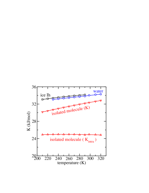
The temperature dependence of $K$ calculated for ice Ih, water, and an isolated molecule with the q-TIP4P/F model potential is represented in Fig. 1. We observe that at a given temperature $K$ is always larger in ice Ih than in water. For a molecule $K$ is the sum of global rotational and translational terms (which are classical contributions at the studied temperatures), and a vibrational term, $K_{intra}$, corresponding to the two OH stretches and the HOH bending mode. In Fig. 1 the temperature dependence of the $K_{intra}$ term has been also shown for the isolated molecule. While $K$ in ice and water increases with temperature, the vibrational term, $K_{intra}$, of the molecule remains nearly constant. This fact indicates that the three intramolecular vibrational modes remain mainly in their ground state in the studied temperature range, while vibrational modes related to the H-bond network display some amount of thermal population of excited states.

The partition of $K$ in ice Ih and water into intra- and intermolecular contributions ($K_{intra}$ and $K_{inter}$) is of interest to quantify the effect of the presence of H-bonds in this observable. The intramolecular term, $K_{intra}$, is attributed to the internal vibrational modes of the molecule, while the intermolecular one, $K_{inter}$, is related to the librational (rotational) and translational motions of the water molecules in the condensed phases. The presence of a H-bond network causes a large broadening of the internal vibrational modes of the water molecule and a shift in the frequencies of their peaks in the infrared absorption spectra.(Habershon et al., 2009) This fact implies that both inter- and intramolecular motions are clearly coupled in the condensed phases of water. Therefore the partition of the total kinetic energy is presented here only as an approximation for didactic purposes in ice and water, and it is not intended to suggest that both types of degrees of freedom may be treated as separable variables.

We estimate $K_{intra}$ in ice Ih and water with the help of a proportionality relation based on the fact that at the studied temperatures $K_{intra}$ is close to the kinetic energy of the ground state associated to three intramolecular modes,$\;K_{GS,intra}$. Particularizing to the case of ice we have,

$$\frac{K_{intra}(ice)}{K_{intra}(molecule)}\approx\frac{K_{GS,intra}(ice)}{K_{GS,intra}(molecule)}\;.$$ (1)

As a rough estimation of the ground state kinetic energy, $K_{GS,intra}$, in either ice, water or an isolated molecule, we employ here a quasi-harmonic approximation, so that a vibrational mode of wavenumber $\omega$ displays a kinetic energy of $\hslash\omega/4$ in its ground state. Thus $K_{GS,intra}$ will be approximated as

$$K_{GS,intra}\approx\frac{\hslash}{4}\left(2\omega_{OH}^{QA}+\omega_{HOH}\right)\;.$$ (2)

The wavenumber $\omega_{OH}^{QA}$ is used here as an estimation of the average wavenumber of the two stretching modes (symmetric and asymmetric) of an isolated water molecule or the corresponding vibrational bands in the condensed phases. $\omega_{OH}^{QA}$ is determined from the equilibrium bond distance, $d_{OH}$, of either ice, water or an isolated molecule, by calculating the second derivative of the potential energy with respect to $d_{OH}$, and by considering the actual O and H masses.(Ramírez and Herrero, 2010) The bending wavenumber is $\omega_{HOH}=$1600 cm^-1. We recall that the bending potential is described by a simple harmonic term in the employed water model.(Habershon et al., 2009) The ground state assumption for $K_{intra}$ in Eq. (1) is further justified by noting that the excitation energy corresponding to the vibrational mode of lowest frequency, $\hslash\omega_{HOH},$ is about seven times larger than the thermal energy, $k_{B}T$, at the highest studied temperature (320 K), and thus the thermal population of excited vibrational modes, as given by a Bose-Einstein statistics,(Moreh et al., 1992; Andreani et al., 2001b) results vanishingly small.

Table 1: Thermal average of the kinetic energy, $K,$ of water and ice Ih at atmospheric pressure and of an isolated water molecule. The results were derived by PIMD simulations at 270 K. The energy $K$ has been partitioned into O- and H-atom contributions ($K_{O},$ $K_{H}$). For water and ice the estimated intramolecular and intermolecular contributions to $K$, $K_{O}$, and $K_{H}$ are also given. For a molecule the classical translational and rotational energy is given as $K_{tr+rot}$. This classical term has been partitioned into O and H components. $d_{OH}$ is the thermal average of the intramolecular OH distance, and $\omega_{OH}^{QA}$ is the quasi-harmonic stretching wavenumber calculated at the distance $d_{OH}$. The last column displays the theoretical results of Ref. Moreh and Nemirovsky, 2010 for ice Ih at 269 K. Kinetic energies are given in kJ/mol (to convert to meV multiply by a factor of 10.37). The standard error in the final digit is given in parenthesis.

	molecule	water	ice Ih	ice Ih
$K$	31.69(5)	33.59(1)	33.93(1)	33.38
$K_{intra}$	24.96(5) (79%)	23.5 (70%)	23.2 (68%)	-
$K_{inter}$	–	10.1 (30%)	10.7 (32%)	-
$K_{tr+rot}$	6.73 (21%)	–	–
$K_{O}$	4.68(1)	5.04(1)	5.09(1)	5.01
$K_{O,intra}$	1.53(1) (33%)	1.4 (29%)	1.4 (27%)	-
$K_{O,inter}$	–	3.6 (71%)	3.7 (73%)	-
$K_{O,tr+rot}$	3.16 (67%)	–	–
$K_{H}$	13.50(2)	14.28(1)	14.42(1)	14.18
$K_{H,intra}$	11.72(2) (87%)	11.0 (77%)	10.9 (76%)	11.2 (79%)
$K_{H,inter}$	–	3.3 (23%)	3.5 (24%)	3.0 (21%)
$K_{H,tr+rot}$	1.78 (13%)	–	–
$d_{OH}$ (Å)	0.957	0.978	0.982
$\omega_{OH}^{QA}$ (cm-1)	3688	3424	3375

The partition of $K$ into $K_{intra}$ and $K_{inter}$ contributions is presented in Table 1 at a temperature of 270 K. For water the intermolecular contribution, $K_{inter}$, is estimated to be 30% (10.1 kJ/mol) of $K$, while for ice Ih this contribution is slightly larger (32%, 10.7 kJ/mol), in agreement with the expectation that H-bonds in ice are stronger than in water.(Chaplin, 2010) We display also the average OH bond distance, $d_{OH}$, and the corresponding quasi-harmonic stretching wavenumber, $\omega_{OH}^{QA}$. The bond distance increases in the order molecule $\ll$ water < ice. We note that x-ray Compton scattering studies of water and ice Ih have shown that the elongation of the OH bond in ice Ih is correlated to its stronger H-bond network,(Nygård et al., 2006) in agreement to the simulation results for $d_{OH}$ and $K_{inter}$ shown in Tab. 1. Our result of $K$ in ice Ih displays a reasonable agreement to a previous calculation that is based on the use of experimental vibrational frequencies assuming a harmonic approximation (see the last column of Tab. 1).(Moreh and Nemirovsky, 2010)

II.3 Kinetic energy of O and H nuclei

Figure 2: Oxygen contribution, $K_{O}$, to the kinetic energy of ice Ih and water as a function of temperature. The classical limit for ice and water amounts to (3/2)$k_{B}T$ per atom. The calculated error bars are smaller than 3$\times 10^{-3}$ kJ/mol. For a given temperature, the difference of $K_{O}$ in ice Ih and water ($\sim 0.05$ kJ/mol) is significantly larger than the error bar.

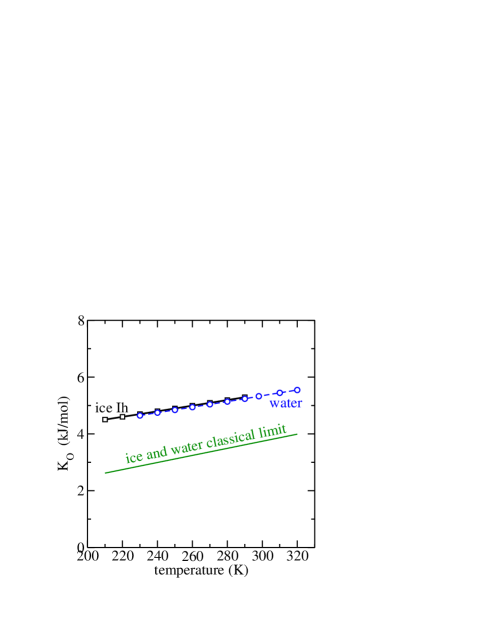
The O nuclei contribution, $K_{O}$, to the kinetic energy is presented in Fig. 2. $K_{O}$ in the condensed phases is significantly larger than its classical limit, i.e., quantum effects related to the oxygen mass are relevant for its kinetic energy. At a given temperature $K_{O}$ is slightly larger in ice Ih than in water (see also the $K_{O}$ values of ice and water at 270 K in Table 1).

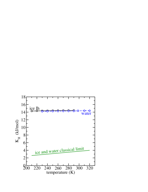
The temperature dependence of $K_{H}$ is presented in Fig. 3 for ice and water. The $K_{H}$ contribution to the kinetic energy is substantially larger than the $K_{O}$ term and it is also much larger than the classical limit, i.e., quantum effects related to their low atomic mass are very important for H atoms. At a given temperature $K_{H}$ is always larger in ice Ih than in water.

Figure 3: Proton contribution, $K_{H}$, to the kinetic energy of ice Ih and water as a function of temperature. The classical limit for the condensed phases corresponds to (3/2)$k_{B}T$ per atom. The calculated error bars are smaller than $5\times 10^{-3}$ kJ/mol. At constant temperature, the difference of $K_{H}$ in ice Ih and water ($\sim 0.1$ kJ/mol) is significantly larger than the error bar.

The partition of $K_{H}$ and $K_{O}$ into intramolecular and intermolecular contributions can be derived by assuming the following proportionality relation for the intramolecular kinetic energy in the condensed phases

$$\frac{K_{H,intra}}{K_{O,intra}}\approx\left(\frac{K_{H,intra}}{K_{O,intra}}\right)_{molecule}\;,$$ (3)

i.e., the ratio $K_{H,intra}/K_{O,intra}$ at a given temperature is assumed to be constant $(\sim 7.7)$ for ice, water, and an isolated molecule. Although we can not provide a theoretical estimation of the error of this assumption, water molecules remain as clearly recognizable entities in the condensed phases at atmospheric pressure, and therefore the intermolecular interactions are not expected to change drastically the constant ratio assumed by Eq. (3). In Table 1 the result of this partition is given at 270 K. For water, the intermolecular contribution to $K_{O}$ is larger than the intramolecular term (71% and 29%, respectively). However in the case of $K_{H}$ in water, the intermolecular contribution (23%, 3.3 kJ/mol) is much lower than the intramolecular term (77%, 11 kJ/mol, corresponding to the two OH stretches and the HOH bending mode). For ice Ih, having a stronger H-bond network than water,(Chaplin, 2010) we find that intermolecular contributions to $K_{O}$ and $K_{H}$ are slightly larger than in water, while the intramolecular contributions are slightly lower.

II.4 Comparison to DINS data

Figure 4: PIMD results obtained with the q-TIP4P/F model for the proton kinetic energy in water and ice Ih are compared to data derived from DINS experiments at temperatures in the range 269-300 K.(Reiter et al., 2004; Pantalei et al., 2008; Reiter et al., 2006; Pietropaolo et al., 2008; Flammini et al., 2009; Pietropaolo et al., 2009b) Also PIMD results for ice Ih derived by ab initio DFT calculations with the SIESTA code are given. Lines are guides to the eyes.

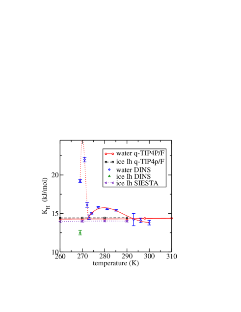
In Fig. 4 our $K_{H}$ results are compared to data derived from DINS experiments.(Reiter et al., 2004; Pantalei et al., 2008; Reiter et al., 2006; Pietropaolo et al., 2008; Flammini et al., 2009; Pietropaolo et al., 2009b) Our calculation for water agrees reasonably well with the data derived from the neutron measurements at 273 K and the three values in the range 290-300 K. However, significant deviations are found in the temperature ranges between 269-272 K and 274-286 K.

The value of $K_{H}$ derived at 271 K from the DINS experiment predicts an excess of 58% (8 kJ/mol) with respect to the room temperature result. This excess was associated to a coherent delocalization of the proton between neighbor oxygen atoms.(Pietropaolo et al., 2009b; Flammini et al., 2009) However, this tentative explanation has been criticized by noting that measured proton momentum distribution implies a contracted proton wave function which is inconsistent with the purported increased proton delocalization. (Soper, 2009) Moreover, coherent delocalization (i.e., tunneling) of a proton is associated to a resonance of the particle between two localized states. A coherent delocalization of the proton at $T_{c}=$271 K would imply that the resonance frequency associated to the coherent process must be large enough to display the following relation to the thermal energy: $\hslash\omega_{c}\gg k_{B}T_{c}$. In other case the quantum coherence would be destroyed by thermal excitations. This inequality should remain valid if $T_{c}$ increases to 273 K, i.e., a slight raise of 2 K should not provide enough thermal energy to destroy a coherent process of wavenumber $\omega_{c}$ for the proton. Therefore, it seems somewhat contradictory that the excess of $K_{H}$ attributed to a coherent process at 271 K disappears completely at 273 K.

An alternative explanation for the large value of $K_{H}$ as a localized proton state at 271 K leads also to an unphysical picture. In this respect, as long as the water molecules maintain their molecular structure, i.e., without a dramatic increase in their stretching frequencies (which has been never observed), the intramolecular contribution to $K_{H}$ must remain below the isolated molecule result of about 11 kJ/mol (see Fig. 3). Therefore an excess as large as 8 kJ/mol in the intramolecular energy seems to be incompatible with the experimental molecular structure of water.

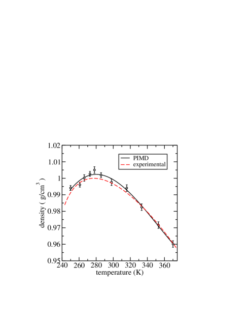
The second maxima in $K_{H}$ derived from the DINS experiments in the temperature range 274-286 K has been attributed to a new structural anomaly of water related to the existence of a maximum in the water density as a function of temperature.(Flammini et al., 2009; Pietropaolo et al., 2009b) This explanation is however not supported by our simulations. The employed water potential is able to reproduce realistically the experimental density maximum of water as a function of temperature (see Fig. 5).(Habershon et al., 2009) In the temperature range between 274-286 K there appears a maximum in the density of water. Both experimental and simulation data agree in the fact that the water density in this temperature range changes by less than 1/1000. Our simulations predict that such a small density change does not affect $K_{H}$ in any significant way (see Fig. 4). However, the excess in $K_{H}$ at 277 K as derived from the DINS experiments amounts to 2.2 kJ/mol with respect to the room temperature value. This excess energy is rather large, and of similar magnitude to the total H-bond network contribution to $K_{H},$ that amounts to about 3.3 kJ/mol for the employed potential model (see Table 1 for our result of $K_{H,inter}$ in water at 270 K, this value remains nearly constant in the studied temperature range). Thus an excess of 2.2 kJ/mol represents, for the employed water model, an increase of 66% in the kinetic energy associated to the intermolecular interaction. We believe that such a large energetic modification should imply a dramatic change of the H-bond network that however has not been observed in any other spectroscopic or thermodynamical data of water around 277 K.

Figure 5: Density of water at 1 atm obtained from PIMD simulations and experimental data from Ref. Kell, 1975. Simulation results correspond to runs of $4\times 10^{6}$ MDS. The continuous line is a cubic fit to the simulation data.

Another discrepancy between our simulations and the DINS analysis of $K_{H}$ is that we find that at isothermal conditions $K_{H}$ is about 0.14 kJ/mol larger in ice than in water. However the DINS value reported for ice(Reiter et al., 2006) at 269 K is much lower ($\sim$ 7 kJ/mol) than that of water(Pietropaolo et al., 2008) at the same temperature.

It is difficult to find a definite explanation for the agreement found between simulation data for $K_{H}$ in water and those derived from neutron scattering at some temperatures (273 K and 290-300 K) and the discrepancies found at other temperatures (269-272 K and 274-286 K) and in the result for ice Ih. Both theoretical and experimental approaches include basic assumptions that might lead to unphysical results. From a theoretical side, the main limitation comes from the use of an empirical water potential. In particular, any dynamic process involving delocalization of protons between different molecules (i.e., breaking and forming of intramolecular OH bonds) can not be described by the employed q-TIP4P/F potential. From the experimental side, the bibliography shows an experimental controversy concerning the validity of the models employed for the data analysis of the DINS experiments at 269 and 271 K.(Soper, 2009; Pietropaolo et al., 2009a) Moreover, the numerical data analysis of the diffraction experiment implies corrections due to the experimental setup (detector position, subtraction of the cell signal) and a numerical integral transform that might be subject to numerical imprecisions. It has been mentioned in the Introduction that numerical reinterpretation of DINS experiments have already happened in recent times.(Reiter et al., 2004; Pantalei et al., 2008)

In the face of this disagreement, the rest of the paper is intended as a consistency check for the ability of the employed empirical potential to reproduce the kinetic energy of the atoms in ice Ih and water. Firstly, we go beyond the empirical potential by presenting results of ab initio DFT simulations.

II.5 Beyond the empirical potential

In Fig. 4 we show the $K_{H}$ results for ice Ih derived from PIMD simulations using atomic forces calculated with the SIESTA code.(Ordejón et al., 1996; Soler et al., 2002) The temperature dependence of $K_{H}$ predicted by the q-TIP4P/F model shows good agreement to the ab initio DFT results. The main difference between both sets of results is that values predicted by the q-TIP4P/F model are $\sim 3\%$ larger than the DFT ones. The origin of this shift is related to a different description of the OH stretching, as evidenced by a normal mode analysis that provides harmonic stretching frequencies about $4\%$ larger in the case of the q-TIP4P/F model. The ab initio data were derived in a small simulation cell (see Sec. II.1). Thus, the finite size error has been estimated by comparing $K_{H}$ values obtained in a small $(2a,a,c)$ and a large $(4a,3\sqrt{3}a,3c)$ supercell (i.e., containing 8 and 288 water molecules, respectively) by using the q-TIP4P/F model. This finite size effect is rather low, the smaller cell shows a $K_{H}$ value $0.3\%$ lower than the larger one. We stress that the q-TIP4P/F potential was parameterized to give correct structure, diffusion coefficient, and infrared absorption frequencies in the liquid state. (Habershon et al., 2009) Therefore the reasonable agreement to the ab initio data found for $K_{H}$ in ice Ih should be considered as a realistic prediction of the empirical potential for a property that was not implicitly built in by the potential parameterization.

In the following Sections we continue our check of the q-TIP4P/F potential by comparing some thermodynamical properties (heat capacity and isotopic shifts) that depend on the kinetic energy of the nuclei with experimental data.

III Heat capacity at 271 K

Table 2: Experimental results for $C_{p}$ of water (Ref. Angell et al., 1982) and ice Ih (Ref. Feistel and Wagner, 2006) are compared with PIMD results at 271 K and 1 atm. The calculated $C_{p}$ has been decomposed into potential ($C_{p1}$ and $C_{p2}$) and kinetic ($C_{p3}$ and $C_{p4}$) energy contributions. The numerical estimation of $C_{p4}$ from the data derived from DINS experiments(Pietropaolo et al., 2008; Flammini et al., 2009; Pietropaolo et al., 2009b) is also given. The employed unit is J mol^-1K^-1.

	water	ice
$C_{p}$ experimental	76.1	37.4
$C_{p}$ PIMD	71.4$\pm 2$	36.1$\pm 0.8$
$C_{p1}(V_{intra})$	-9.0$\pm 0.4$	-7.4$\pm 0.2$
$C_{p2}(V_{inter})$	66.3$\pm 1$	31.6$\pm 0.5$
$C_{p3}(K_{O})$	10.3$\pm 0.2$	9.9$\pm 0.05$
$C_{p4}(K_{H})$	3.7$\pm 0.2$	2.0$\pm 0.05$
$C_{p4}(K_{H},$ DINS)	$-10^{4}$	-

The enthalpy, $H$, calculated with the employed water model can be expressed as

$$H=V_{intra}+V_{inter}+K_{O}+K_{H}+PV\;,$$ (4)

where the first four summands give the internal energy as a sum of potential ($V$) and kinetic energy ($K$) terms and the potential energy is partitioned into a sum of intramolecular ($V_{intra})$ and intermolecular ($V_{inter})$ contributions. We have fitted our PIMD results for the enthalpy of ice and water to a quadratic function of temperature in the range 250-290 K. Then the constant pressure heat capacity

$$C_{p}=\left(\frac{\partial H}{\partial T}\right)_{P}\;$$ (5)

has been calculated at 271 K by performing the temperature derivative of the fitted function. The results are presented in Table 2 and compared to experimental data. The employed water model provides realistic values of $C_{p}$ for both water and ice at 271 K. The deviation with respect to experiment amounts to about 6% in water and to 4% in ice Ih, with simulated values lower than experimental ones. Note that the experimental heat capacity of ice Ih is nearly one half of that of water, a fact that is reasonably reproduced by the simulations. This overall agreement encourages us to analyze separately the potential ($C_{p1},C_{p2}$) and kinetic ($C_{p3},C_{p4}$) energy contributions to $C_{p}$, as derived from the temperature derivative of the first four summands in Eq. (4). At atmospheric pressure the temperature derivative of the $PV$ term gives a vanishingly small contribution to $C_{p}$.

The four contributions to the calculated $C_{p}$ have been summarized in Table 2. We note that the contribution $C_{p1}$ of the intramolecular potential energy ($V_{intra}$) is negative for both water and ice Ih. This result is an anharmonic effect related to the reduction of the $d_{OH}$ distance with increasing temperature, a fact that has been experimentally reported in water,(van Panthaleon van Eck et al., 1958; Nygård et al., 2006) and that is reproduced by the employed model potential. The largest contribution ($C_{p2}$) to the heat capacity comes from the potential energy of the H-bond network, $V_{inter}$. $C_{p2}$ amounts to 93% of the calculated $C_{p}$ in water and to 88% in ice, a result in line to the expectation that the high heat capacity of water is a consequence of its H-bond network. Kinetic energy contributions ($C_{p3},C_{p4}$) are comparatively much lower. $C_{p3}$, derived from the temperature derivative of the kinetic energy $K_{O}$, is several times larger than $C_{p4}$, that is derived from $K_{H}$. In particular, we find that $C_{p4}$ amounts to less than 4 J mol^-1K^-1 (5% of the calculated $C_{p}$) in water.

The last line of Table 2 summarizes the value of $C_{p4}$, as derived from the temperature derivative of the $K_{H}$ values obtained from the DINS experiments, that were plotted in Fig. 4. This contribution is negative and its absolute value ($\sim 10^{4}$J mol^-1K^-1) is several orders of magnitude larger than the experimental heat capacity. Both sign and magnitude of this estimation of $C_{p4}$ seem to be unphysical and incompatible with the experimental $C_{p}$ data at 271 K. This fact let us to question if the maximum in $K_{H}$ derived from the DINS analysis around 270 K (see Fig. 4) corresponds to any real physical effect.

IV Isotopic shift in the melting temperature

Figure 6: Schematic representation of the free energy difference, $\Delta G$, between solid and liquid phases of water as a function of temperature at constant pressure. The continuous line represents $\Delta G_{H}$ for phases containing the isotope ¹H and the melting temperature of the solid is $T_{H}$. Upon isotopic substitution of H by deuterium, the free energy curve is shifted to the broken one, $\Delta G_{D}$. At given temperature the shift of $\Delta G_{D}$ with respect to $\Delta G_{H}$ (shown by an arrow at the temperature $T_{H}$) can be calculated by the definite integral in Eq. (7). A normal isotopic shift implies that the melting temperature of the heavier isotope is higher ($T_{D}>T_{H}$).

For ice Ih at atmospheric pressure experimental isotopic shifts indicate that heavier isotopes display higher melting temperatures. Thus deuterated ice Ih melts at a temperature 3.8 K higher than normal ice, while the isotopic shift for tritiated ice amounts to 4.5 K. Also H₂¹⁸O melts at a temperature 0.3 K higher than ice Ih made of normal H₂¹⁶O. Isotopic shifts in the melting temperature are a consequence of the dependence of the Gibbs free energy, $G$, on the isotope mass. At constant ($T$,$P)$, this dependence results to be a function of the kinetic energy of the isotope. Thus if $G_{H}$ is the Gibbs free energy of a water phase containing ¹H atoms, the free energy of the corresponding deuterated phase, $G_{D}$, is given by the following relation(Ramírez and Herrero, 2010)

$$G_{D}=G_{H}-\int_{m_{H}}^{m_{D}}\frac{dm}{m}K_{H}(m)\;,$$ (6)

where $m_{H}$ and $m_{D}$ are the H and deuterium (D) masses, and $K_{H}(m)$ is the thermal average of the kinetic energy of a H isotope with mass $m$. Note that the mass $m$ appears as an auxiliary variable in Eq. (6) and corresponds to a real isotope only at the integration limits ($m_{H},m_{D}$). The Gibbs free energy difference, $\Delta G=G_{s}-G_{l}$, between the solid ($s$) and liquid ($l)$ phases at constant $(T,P)$ can be expressed from Eq. (6) as

$$\Delta G_{D}=\Delta G_{H}-\int_{m_{H}}^{m_{D}}\frac{dm}{m}\Delta K_{H}(m)\;,$$ (7)

where

$$\Delta K_{H}(m)=K_{H,s}(m)-K_{H,l}(m)\;.$$ (8)

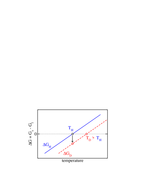
$K_{H,s}(m)$ is the isotope kinetic energy in the solid and $K_{H.l}(m)$ the corresponding quantity in the liquid phase. A schematic representation of the free energy difference $\Delta G_{H}$ at constant pressure is shown in Fig. 6 as a function of $T$. At the melting temperature, $T_{H}$, the free energy of both phases must be identical and $\Delta G_{H}$ vanishes. At temperatures below $T_{H}$ we find that $\Delta G_{H}<0$, i.e., the solid is the thermodynamically stable phase as it displays lower free energy than the liquid. However, for $T>T_{H}$ one finds $\Delta G_{H}>0$ and then the stable phase is the liquid one. The isotope effect in the melting temperature can be obtained by calculating $\Delta G_{D}$ with the help of Eq. (7). A normal isotope effect implies that the definite integral in Eq. (7) takes a positive value. Thus at constant temperature $\Delta G_{D}$ becomes smaller than $\Delta G_{H}$ obtaining the schematic result represented in Fig. 6. Note that the melting point for the heavier isotope, $T_{D}$ (where $\Delta G_{D}\equiv 0$), is shifted towards higher temperatures.

We conclude that it is the sign associated to the value of the definite integral in Eq. (7) what determines if the isotope effect in the melting temperature is normal (i.e., higher melting temperature for a heavier isotope mass if the sign is positive) or it is an inverse isotope effect (lower melting point for a heavier isotope mass if the sign is negative). A sufficient (but not necessary) condition to obtain a normal isotope effect is that

$$\Delta K_{H}(m)>0;\quad\mathrm{for\;}m_{H}\leq m\leq m_{D}$$ (9)

i.e., the isotope kinetic energy is larger in the solid than in the liquid phase for the isotope masses $m$ in the studied interval.

Our simulations show that the condition in Eq. (9) is satisfied for the isotopic substitution of H by either deuterium or tritium. The analogous condition, $\Delta K_{O}(m)>0$, is also satisfied for the isotopic substitution of ¹⁶O by ¹⁸O, with $m(^{16}\mathrm{O})\leq m\leq m(^{18}\mathrm{O})$. Thus the employed water model predicts normal isotopic shifts in the melting temperature upon isotopic substitution of either ¹H or ¹⁶O by a heavier isotope, in agreement to experiment. Detailed results for deuterated and tritiated phases have been presented elsewhere.(Ramírez and Herrero, 2010) The values collected in Table 1 at 270 K show that for hydrogen we get the value $\Delta K_{H}(m_{H})=0.14$ kJ/mol, i.e., $K_{H}$ is larger in the solid than in the liquid, while for ¹⁶O we find than $K_{O}$ is 0.05 kJ/mol larger in ice than in water.

The $K_{H}$ results derived from DINS data for water and ice Ih at 269 K give $\Delta K_{H}(m_{H})=-6.7$ kJ/mol, i.e., $K_{H}$ is much lower in ice than in water. Note that here the inequality of Eq. (9) is not satisfied for $m_{H}$. This fact implies that a small increase in the mass of hydrogen would produce an inverse isotope effect in the melting temperature. This behavior for $m_{H}$ does not imply an inverse isotope effect for deuterium, because the latter effect is determined by the definite integral in Eq. (7) that involves all masses $m$ with $m_{H}\leq m\leq m_{D}$. However, the value of $\Delta K_{H}(m_{H})=-6.7$ kJ/mol at 269 K derived from the DINS analysis contrasts in sign and magnitude with our result of $\Delta K_{H}(m_{H})=0.14$ kJ/mol. We stress that the employed potential model provides a realistic prediction of the isotopic shift in the melting temperature of ice, a fact that let us expect that our calculation of $\Delta K_{H}(m_{H})$ must be also reasonably realistic.(Ramírez and Herrero, 2010) This consideration rises further doubts about the physical significance of the maximum in $K_{H}$ derived from the DINS analysis for liquid water around 270 K.

V Conclusions

Quantum PIMD simulations at atmospheric pressure show that the q-TIP4P/F model provides realistic results for several thermodynamic properties of water and ice Ih. In particular, satisfactory agreement to experiment has been found in the dependence of the water density with temperature,(Habershon et al., 2009) the isotopic shifts in the melting temperature of deuterated and tritiated ice,(Ramírez and Herrero, 2010) and the constant-pressure heat capacity of water and ice Ih at 271 K. In the present paper we have focused on the calculation of the proton kinetic energy, $K_{H}$, and its comparison to available data derived from the analysis of neutron scattering experiments,(Reiter et al., 2004; Pantalei et al., 2008; Reiter et al., 2006; Pietropaolo et al., 2008; Flammini et al., 2009; Pietropaolo et al., 2009b) and also to results based on ab initio DFT simulations.

This comparison has shown a remarkable agreement between the computational model and DINS data for water at some temperatures (273 K and in the range 290-300 K), but a strong disagreement at other similar temperatures (in the range 269-272 K and 274-286 K). Our simulations predict that $K_{H}$ remains nearly constant in the temperature range where DINS data are available at atmospheric pressure. On the contrary, $K_{H}$ values derived from the scattering experiments display a remarkable temperature dependence with two maxima at 270 K and 277 K. This strong temperature dependence and, particularly, the large DINS value reported for $K_{H}$ at 271 K (58% larger than at room temperature) are the main discrepancies found with our results for water. Our simulations predict that under isothermal conditions $K_{H}$ is larger in ice than in water while the values derived from DINS data at 269 K forecast that $K_{H}$ is much lower in ice Ih than in water.

In the face of the discrepancies found between our simulation results for $K_{H}$ and those derived from neutron scattering experiments, we have related $K_{H}$ to other thermodynamic properties pursuing to gain a deeper understanding of the implication of such differences. We find that the maximum in the density of water is not related to any significant effect in the proton kinetic energy at atmospheric pressure. In the analysis of $C_{p}$ our simulations display reasonable results for both water and ice Ih at 271 K. The $K_{H}$ contribution to $C_{p}$ amounts to about 4 J mol^-1K^-1 in water (5% of $C_{p}$ ). However, the temperature dependence of $K_{H}$ as derived from DINS experiments leads to a dramatic negative contribution to $C_{p}$ of about $-10^{4}$ J mol^-1K^-1. This value can not be directly compared to experimental data, but both its sign and magnitude seem to be outside any reasonable physical boundary. At this point it is clear that further independent experiments and theoretical calculation are necessary to clarify this question.

The calculated values of $K_{O}$ and $K_{H}$ in water and ice at isothermal conditions show that the largest results are always associated to the solid phase. This fact determines the sign of the isotopic shifts in the melting temperature upon isotopic substitution of either H or O atoms. In both cases the model predictions are in agreement to experiment. The temperature dependence of $K_{H}$ in ice Ih has shown satisfactory agreement to results derived from PIMD simulations based on ab initio DFT calculations using the SIESTA code.(Ordejón et al., 1996; Soler et al., 2002)

Summarizing, it is clear that an empirical potential model of water can not reproduce quantitatively all thermodynamic properties of the real system. However, it is the combined analysis of several thermodynamic properties such as the proton kinetic energy $K_{H}$, the intramolecular and intermolecular contributions to $K_{H}$, the heat capacity $C_{p}$, the isotopic shifts in melting temperatures, and the density-temperature curve of water, what let us believe that the employed model provides realistic results for the temperature dependence of $K_{H}$ in water and ice Ih at atmospheric pressure.