Toward a Realistic Pulsar Magnetosphere

Abstract

We present the magnetic and electric field structures as well as the currents and charge densities of pulsar magnetospheres which do not obey the ideal condition, ${\bf E\cdot B=0}$. Since the acceleration of particles and the production of radiation requires the presence of an electric field component parallel to the magnetic field, ${\bf E}_{\parallel}$, the structure of non-Ideal pulsar magnetospheres is intimately related to the production of pulsar radiation. Therefore, knowledge of the structure of non-Ideal pulsar magnetospheres is important because their comparison (including models for the production of radiation) with observations will delineate the physics and the parameters underlying the pulsar radiation problem. We implement a variety of prescriptions that support nonzero values for ${\bf E}_{\parallel}$ and explore their effects on the structure of the resulting magnetospheres. We produce families of solutions that span the entire range between the vacuum and the (ideal) Force-Free Electrodynamic solutions. We also compute the amount of dissipation as a fraction of the Poynting flux for pulsars of different angles between the rotation and magnetic axes and conclude that this is at most 20-40% (depending on the non-ideal prescription) in the aligned rotator and 10% in the perpendicular one. We present also the limiting solutions with the property $J=\rho c$ and discuss their possible implication on the determination of the “on/off” states of the intermittent pulsars. Finally, we find that solutions with values of $J$ greater than those needed to null ${\bf E}_{\parallel}$ locally produce oscillations, potentially observable in the data.

1 Introduction

Pulsars are extraordinary objects powered by magnetic fields of order $10^{12}$ G anchored onto neutron stars rotating with periods $\sim 10^{-3}-10$ s. These fields mediate the conversion of their rotational energy into MHD winds and the acceleration of particles to energies sufficiently high to produce GeV photons. Their electromagnetic emission is quite complex and ranges from the radio to the multi-GeV $\gamma-$ray regime.

Pulsar radiation has been the subject of many studies since their discovery; however, despite such a multi-decade effort by a large number of researchers its details are not fully understood. There are several reasons for this. On the observational side, the sensitivity of the $\gamma-$ ray instruments (the band where most of the pulsar radiation power is emitted) has become adequate for the determination of a significant number of pulsar spectra only recently. Since its launch in 2008, the Fermi Gamma-Ray Space Telescope has revolutionized pulsar physics by detecting nearly 90 $\gamma-$ray pulsars so far, with a variety of well-measured light curves. On the theoretical side, the structure of the pulsar magnetosphere, even for the simplest axisymmetric case, remained uncertain for a long time. The modeling of pulsar magnetospheres has seen rapid advancements only very recently.

The original treatment of the non-axisymmetric rotating stellar dipole in vacuum (Deutsch, 1955) established the presence of an electric field component, ${\bf E}_{||}$, parallel to the magnetic field on the star’s surface. Then Goldreich & Julian (1969) suggested that this component of the electric field would pull charges out of the pulsar, opening up magnetic field lines that cross the Light Cylinder (hereafter LC), to produce an MHD wind with currents flowing out of and into the neutron star polar cap. The charge density needed to achieve this is known as the Goldreich - Julian density $\rho_{\rm GJ}$; an associated current density $J_{\rm GJ}=c\rho_{\rm GJ}$ is obtained if we allow these charges to move outward at nearly the speed of light.

Following the work of Goldreich & Julian (1969), a number of attempts were made to produce the structure of the pulsar magnetosphere. Thus, Scharlemann & Wagoner (1973) were able to reduce the structure of the axisymmetric magnetosphere to a single equation for the poloidal magnetic flux, the so-called pulsar equation. However an exact solution of this equation that would produce the magnetic field structure across the LC was missing for almost 3 decades (for a review of the problems and the various attempts to produce a consistent pulsar magnetosphere, even in the axisymmetric case, see Michel, 1982). In fact, the inability of models to determine the magnetospheric structure across the LC led people to speculate that its structure is not smooth across this surface and assumed that the observed radiation is the result of magnetic field discontinuities across the LC (Mestel & Shibata, 1994).

The structure of the axisymmetric pulsar magnetosphere within Force Free Electrodynamics (hereafter FFE) (i.e. assuming that the only surviving component of the electric field is that perpendicular to the magnetic field, or equivalently that ${\bf E\cdot B=0}$) was given by Contopoulos, Kazanas, & Fendt (1999) (hereafter CKF) who used an iterative procedure to determine the current distribution on the LC so that the magnetic field lines should cross this surface smoothly. Besides allowing a smooth transition of the magnetic field lines across the LC, this solution also resolved the issue of the current closure in pulsar magnetospheres: The current starts near the polar axis and closes, for $R>R_{\rm LC}$ (here $R_{\rm LC}$ is the radius of the LC), mainly along an equatorial current sheet (allowing also a small amount of return current at a finite height above it). For $R<R_{\rm LC}$ the flow is mainly along the separatrix of the open and closed field lines. The axisymmetric solution has since been confirmed and further studied by several others (Gruzinov, 2005; Timokhin, 2006; Komissarov, 2006; McKinney, 2006), in particular with respect to its properties near the Y-point (the intersection of the last closed field line and the LC; Uzdensky, 2003).

The first non-axisymmetric (3D), oblique rotator magnetosphere was presented by Spitkovsky (2006), who used a time-dependent numerical code to advance the magnetic and electric fields under FFE conditions to steady state. These simulations confirmed the general picture of current closure established by the CKF solution and produced a structure very similar to that of CKF in the axisymmetric case. Similar simulations were performed by Kalapotharakos & Contopoulos (2009) who, using a Perfectly Matched Layer (hereafter PML) at the outer boundary of their computational domain, were able to follow these simulations over many stellar rotation periods. In general, the 3D magnetosphere, just like the axisymmetric one, consists of regions of closed and open field lines with a large scale electric current circuit established along open magnetic field lines. In the 3D case, the current sheet needed for the global current closure is in fact undulating, as foreseen in the kinematic solution of Bogovalov (1999). As shown by recent simulations, the undulating current sheet structure is stable at least to distances of $10R_{LC}$ and for several stellar rotation periods (Kalapotharakos, Contopoulos, & Kazanas, 2011).

The FFE solutions presented so far, by construction, do not allow any electric field component parallel to the magnetic field ${\bf B}$ (${\bf E\cdot B=0}$); as such they do not provide the possibility of particle acceleration and the production of radiation, in disagreement with observation. Nonetheless, models of pulsar radiation have been constructed assuming either a vacuum dipole geometry, or the field line geometry of the FFE magnetosphere. Polar cap particle acceleration, $\gamma-$ray emission and the formation of pair cascades were discussed over many years as a means of accounting for the observed high-energy radiation (Ruderman & Sutherland, 1975; Daugherty & Harding, 1996). However, measurements by Fermi of the cutoff shape of the Vela pulsar spectrum (Abdo et al., 2009b) has ruled out the super-exponential shape of the spectrum predicted by polar cap models due to the attenuation of pair production. Models placing the origin of the high-energy emission in the outer magnetosphere or beyond are now universally favored. Slot gap models (Muslimov & Harding, 2004; Harding et al., 2008), with acceleration and emission in a narrow layer along the last open field line from the neutron star surface to near the LC, and outer gap models (Romani & Yadigaroglu, 1995; Romani, 1996; Takata et al., 2007) produce light curves and spectra in first-order agreement with the Fermi data (Romani & Watters, 2010; Venter, Harding, & Guillemot, 2009). All of the above models assume a retarded vacuum magnetic field. There are also kinematic models of pulsar emission derived by injecting photons along the magnetic field lines of either the FFE magnetosphere (Bai & Spitkovsky, 2010b) or those of the vacuum field geometry (Bai & Spitkovsky, 2010a), or along the electric current near the equatorial current sheet where the ratio $J/\rho c\rightarrow 1$ in FFE (Contopoulos & Kalapotharakos, 2010). These models also produce light curves in broad agreement with observations. However, fits of Fermi data light curves with slot gap and outer gap models in FFE geometry are less favorable than those for the vacuum dipole geometry (Harding et al., 2011).

While FFE magnetospheres do not allow for particle acceleration, they do, however, provide a global magnetospheric structure consistent with the boundary conditions on the neutron star surface (a perfect conductor), a smooth transition through the LC and the establishment of a large scale MHD wind. They also determine both the currents and the sign of the charges that flow in the magnetosphere. However, they do not provide any information about the particle production that might be necessary to support the underlying charge conservation and electric current continuity. This was apparent already in the CKF solution and was also noted in Michel (1982): There are regions, most notably the intersections of the null charge surface with open magnetic field lines and the region near the neutral (Y) point of the LC where the FFE charge density changes sign along an open field line (along which particles are supposed to flow freely). The numerical FFE solution has no problem in these regions because it can simply supply at will the charges necessary for current closure and for consistency with the global boundary conditions. This, however, requires sources of electron-positron pairs at the proper regions and of the proper strength. Even though the FFE treatment of the pulsar magnetosphere involves no such processes, these must be taken into account self-consistently. Viewed this way, pulsar radiation is the outcome of the “tension” between the boundary conditions imposed by the global magnetospheric structure and the particle production necessary for charge conservation and electric current continuity.

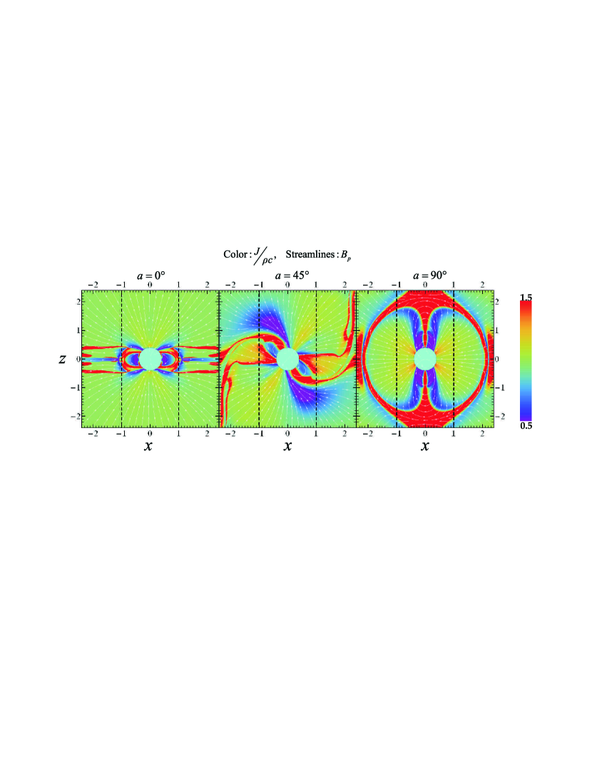
Figure 1: The FFE solutions for the inclination angles $a$ indicated in the figure. Each panel shows the poloidal magnetic field lines (white colored lines) and the ratio $J/\rho c$ in the color scale shown in the figure. We note that the color scale saturates below the value 0.5 and above 1.5 so that details around the value 1 become evident. The dashed vertical lines denote the Light Cylinder (LC). The length unit is equal to $R_{\rm LC}$. We observe that the magnetic field lines open beyond the LC. The fraction of the polar cap region with space-like currents ($J/\rho c\geq 1$) increases with $a$ so that, while in the aligned rotator almost the entire polar cap is filled with time-like currents ($J/\rho c\leq 1$), in the perpendicular rotator the entire polar cap is filled with space-like currents ($J/\rho c\geq 1$).

In Figs. 1a,b,c we present the structure of the FFE magnetosphere on the poloidal plane $\boldsymbol{\mu}-\mathbf{\Omega}$ for inclination angles $a=(0^{\circ},45^{\circ},90^{\circ})$. These figures depict the poloidal magnetic field lines and in color the value of $J/\rho c$. The vertical dashed lines denote the position of the LC. In the axisymmetric case the value of $J/\rho c$ is less than one in most space and exceeds this value only in the null surfaces and the separatrix between open and closed field lines. The value 1 of this ratio is significant because it denotes the maximum current density for carriers of single sign charge. Values of this ratio greater than 1, by necessity denote the presence of both positive and negative charges moving in opposite directions. For $a\simeq 0$, $J/\rho c<1$ in most of the polar cap region, however, as the value of inclination $a$ increases so does the size of regions with $J/\rho c>1$; in the perpendicular rotator we see clearly that $J/\rho c>1$ over the entire polar cap region.

With the above considerations in mind, the question that immediately arises is how would the structure of the pulsar magnetosphere and the consequent production of radiation be modified, if the ideal condition, namely ${\bf E\cdot B=0}$, were dropped. This is the subject of the present work. A successful magnetospheric configuration (solution) should be able to address the following questions: a) Where does particle acceleration take place? b) How close are these processes to a steady state? c) Is the ensuing particle acceleration and radiation emission consistent with the Fermi pulsar observations?

Unfortunately, while the ideal condition is unique, its modifications are not. The evolution equations require a relation between the current density $\mathbf{J}$ and the fields, i.e. a form of Ohm’s law, a relation which is currently lacking. Meier (2004) proposed a generalization of Ohm’s law in plasmas taking into account many effects (e.g. pressure, inertia, Hall). However, in the present case we are in need of a macroscopic expression for Ohm’s law which would be also everywhere compatible with the microphysics self-consistently, a procedure that might involve Particle in Cell (PIC) techniques, well beyond the scope of this paper. For this reason, the present work has a largely exploratory character. A number of simple prescriptions are invoked which lead to magnetospheric structures with values of ${\bf E}_{||}\neq 0$. The global electric current and electric field structures are then examined with emphasis on the modifications of the corresponding FFE configuration. We are presently interested only in the broader aspects of this problem, deferring more detailed calculations to future work. In particular, the general compatibility of the ${\bf E}_{||}$ magnitude with the values needed to produce (through pair production) self-consistent charge and current densities from the plasma microphysics will not be discussed in the present paper. The contents of the present paper are as follows: In §2 we discuss the different modifications in the expression for the electric current that we apply in order to obtain non-Ideal solutions. In §3 we present our results and the properties of the new solutions. In §4 we give particular emphasis to specialized solutions that obey certain global conditions. Finally, in §5 we present our conclusions.

2 Non-Ideal Prescriptions

In the FFE description of pulsal magnetospheres Spitkovsky (2006) and Kalapotharakos & Contopoulos (2009) solved numerically the time dependent Maxwell equations

$$\frac{\partial\mathbf{B}}{\partial t} =-c\boldsymbol{\nabla}\times\mathbf{E}$$ (1)

$$\frac{\partial\mathbf{E}}{\partial t} =c\boldsymbol{\nabla}\times\mathbf{B}-4\pi\mathbf{J}$$ (2)

under ideal force-free conditions

$$\mathbf{E\cdot B}=0,\ \ \rho\mathbf{E+\frac{1}{c}J\times B}=0,$$

where $\rho=\mathbf{\nabla\cdot E}/(4\pi)$. The evolution of these equations in time requires in addition an expression for the current density $\mathbf{J}$ as a function of $\mathbf{E}$ and $\mathbf{B}$. This is given by

$$\mathbf{J}=c\rho\frac{\mathbf{E}\times\mathbf{B}}{B^{2}}+\frac{c}{4\pi}\frac{\mathbf{B\cdot\nabla\times B-E\cdot\nabla\times E}}{B^{2}}\mathbf{B}$$ (3)

(Gruzinov, 1999). The second term in Eq. (3) ensures that the condition $\mathbf{E\perp B}$ (the ideal condition) is preserved during the time evolution. However, this term introduces numerical instabilities since it involves spatial derivatives of both fields. Thus, Spitkovsky (2006) implemented a scheme that evolves the fields considering only the first term of Eq. (3), and at the end of each time step “kills” any developed electric field component parallel to the magnetic field $(\mathbf{E_{||}})$. In the case of non-Ideal status, the $\mathbf{E}_{\parallel}=0$ condition does not apply anymore and electric field components parallel to the magnetic field are allowed. However, while in FFE the prescription that determines the value of $\mathbf{E_{||}}$ is unique (it is equal to zero), there is no unique prescription in the non-Ideal case. Below we enumerate the non-Ideal prescriptions that we consider in the present study:

(A) The above implementation of the ideal condition, hints at an easy generalization that leads to non-Ideal solutions: One can evolve Eqs. (1) & (2), using only the first term of the FFE current density (Eq. 3), and at each time step keep only a certain fraction $b$ of the $\mathbf{E_{||}}$ developed during this time instead of forcing it to be zero. In general the portion $b$ of the remaining $\mathbf{E_{||}}$ can be either the same everywhere or variable (locally) depending on some other quantity (e.g. $\rho,J$). As $b$ goes from 0 to 1 the corresponding solution goes from FFE to vacuum. In this case an expression for the electric current density is not given a priori, and $\mathbf{J}$ can be obtained indirectly from the expression

$$\mathbf{J}=\frac{1}{4\pi}\left(c\boldsymbol{\nabla}\times\mathbf{B}-\frac{\partial\mathbf{E}}{\partial t}\right)$$ (4)

(B) Another way of controlling $\mathbf{E_{||}}$ is to introduce a finite conductivity $\sigma$. In this case we replace the second term in Eq. (3) by $\sigma\mathbf{E_{||}}$ and the current density reads

$$\mathbf{J}=c\rho\frac{\mathbf{E}\times\mathbf{B}}{B^{2}}+\sigma\mathbf{E_{||}}$$ (5)

Note that Eq. (5) is related to but is not quite equivalent to Ohm’s law which is defined in the frame of the fluid. Others (Lyutikov, 2003; Li, Spitkovsky, & Tchekhovskoy, 2011) implemented a different version closely related to Ohm’s law. The problem is that the frame of the fluid is not well defined in our problem. Moreover, it is not a priori known neither that a single form of Ohm’s law is applicable in the entire magnetosphere, nor that the conductivity corresponding to each such form of Ohm’s law should be constant (e.g. in regions where pair production takes place). This is why we chose a simpler expression, which turns out to yield results qualitatively very similar to other formulations based on Ohm’s law. As is the case in prescription (A) with the parameter $b$, here too, as $\sigma$ ranges from $\sigma=0$ to $\sigma\rightarrow\infty$ we obtain a spectrum of solutions from the vacuum to the FFE, respectively. We note that even though the vacuum and FFE solutions are unambiguously defined limiting cases, there is an infinite number of paths connecting them according to how $\sigma$ depends on the local physical parameters of the problem ($\rho,E,B$ etc.).

(C) It has been argued (Lyubarsky, 1996; Gruzinov, 2007; Lyubarsky, 2008) that regions corresponding to space-like currents $(J/\rho c>1)$ are dissipative due to instabilities related to counter streaming charge flows. Moreover, the space-like current regions should trace the pair production areas (i.e. dissipative areas). Gruzinov (2007) proposed a covariant formulation for the current density that introduces dissipation only in the space-like regions while the time-like regions remain non-dissipative. The current density expression in the so called Strong Field Electrodynamics (hereafter SFE) reads

$$\mathbf{J}=\frac{c\rho\mathbf{E\times B}+(c^{2}\rho^{2}+\gamma^{2}\sigma^{2}E_{0}^{2})^{1/2}(B_{0}\mathbf{B}+E_{0}\mathbf{E})}{B^{2}+E_{0}^{2}}$$ (6)

where

$$B_{0}^{2}-E_{0}^{2}=\mathbf{B^{2}-E^{2}},\;B_{0}E_{0}=\mathbf{E\cdot B},\;E_{0}\geq 0$$ (7)

$$\gamma^{2}=\frac{B^{2}+E_{0}^{2}}{B_{0}^{2}+E_{0}^{2}}$$ (8)

and $\sigma$ is a function of $E_{0},B_{0}$ with dimensions of conductivity (inverse time). The expression for $\mathbf{J}$ (Eq. 6) produces either a space-like $(\sigma>0)$ or a null $(\sigma=0)$ current. Note that this treatment precludes time-like currents. Such currents do exist but they are only effectively time-like: the current $J$, along with $E_{\parallel}$, fluctuates continuously, so that while $J$ is locally greater than (or equal to) $\rho c$ its average value is less than that, i.e. $\langle J\rangle<\rho c$. This behavior is captured by our code and is manifest by the continuously changing direction of the parallel component of the electric field along and against the magnetic field direction (Gruzinov, 2008, 2011).

In prescriptions (A) and (B) above, care must be taken numerically so that the resulting value of $E_{\perp}$ (defined as $|{\bf E}-{\bf E}_{\parallel}|$) be less than B. Violation of this condition usually happens in the current sheet where the value of B goes to zero. We note that the presence of the $E_{0}$ term in the denominator of the SFE prescription (Eq. 6) and of the prescription of $\mathbf{J}$ used by Li et al. (2011) indeed prevents the denominator from going to zero and alleviates this issue in the current sheet regions. However, alleviation of this problem does not guarantee that all treatments that include this $E_{0}$ term converge to the same solution or that even produce the same dissipation rates in the current sheet. Thus, the solutions and in particular the dissipation rates of SFE and that of Li et al. (2011) can be quite different.

All the simulations that are presented below have run in a cubic computational box 20 times the size of the LC radius $R_{\rm LC}$, i.e $[-10R_{\rm LC}\ldots 10R_{\rm LC}]^{3}$. Outside this area we implemented a PML layer that allows us to follow the evolution of the magnetosphere for several stellar rotations (Kalapotharakos & Contopoulos, 2009). The adopted grid cell size is $0.02R_{\rm LC}$, the stellar radius has been considered at $r_{\star}=0.3R_{\rm LC}$, and all simulations were run for 4 full stellar rotations to ensure that a steady state has been achieved.

3 Results

We have run a series of simulations using prescription (B) that cover a wide range of $\sigma$ values. In Fig. 2a we present the values of the Poynting flux $L$ integrated over the surface of the star for the $a=0^{\circ}$ (aligned; red), $a=45^{\circ}$ (green) and $a=90^{\circ}$ (perpendicular; blue) versus $\sigma$ in log-linear scale. The two solid horizontal line segments of the same color denote in each case ($a=0^{\circ},45^{\circ},90^{\circ}$) the corresponding limiting values of the Poynting flux for the FFE and the vacuum solutions, respectively. The Poynting flux as a function of the inclination angle $a$ for the vacuum and the FFE solutions reads

$$L=\begin{cases}\dfrac{2}{3}\dfrac{\mu^{2}\Omega^{4}}{c^{3}}\sin^{2}a&\text{Vacuum}\\ \\ \dfrac{\mu^{2}\Omega^{4}}{c^{3}}(1+\sin^{2}a)&\text{FFE}\end{cases}$$ (9)

where $\mu,\Omega$ are the magnetic dipole moment and the rotational frequency of the star, respectively. This means that for a specific value of $a$ the corresponding value of the Poynting flux (spin-down rate) of each non-Ideal modification should lie between the two values of Eq. (9). Thus, Fig. 2a shows that for the perpendicular rotator (and any case with $a\neq 0$) the ratio of the Poynting flux over that of the vacuum reaches near 1 for low values of $\sigma~{}(\sigma/\Omega\mathrel{\raise 1.29167pt\hbox{$<$}\mkern-14.0mu\lower 2.58334pt\hbox{$\sim$}}0.01$; for $a=0$ this is true only for $\sigma\rightarrow 0$). In Fig. 2b we plot for these simulations the corresponding dissipation power

$$\dot{E}_{D}=\int_{r_{1}<r<r_{2}}\mathbf{J}\cdot\mathbf{E}\ {\rm d}V=\frac{1}{4\pi}\int_{r_{1}<r<r_{2}}\sigma E_{\parallel}^{2}\ {\rm d}V$$ (10)

taking place within the volume bounded by the spheres $r_{1}=0.3R_{LC}$, i.e just above the star surface, and $r_{2}=2.5R_{LC}$, versus $\sigma$. We see that the energy losses due to dissipation exhibit a maximum that occurs at intermediate values of $\sigma~{}(\sigma/\Omega\simeq 1)$ for $a=90^{\circ}$ and at higher values of $\sigma$ as the inclination angle $a$ decreases. The dissipation power $\dot{E}_{D}$ goes to 0 as $\sigma$ goes either towards 0 or $\infty$ since both the vacuum ($\sigma=0$) and FFE ($\sigma\rightarrow\infty$) regimes are (by definition) dissipationless. We note that despite the fact that the Poynting flux (on the stellar surface) varies significantly with $\sigma$, the corresponding energy loss due to dissipation is limited and it never exceeds the value $\simeq 0.14\mu^{2}\Omega^{4}/c^{3}$. The surface Poynting flux reflects the spin down rate while the dissipative energy loss within the magnetosphere reflects the maximum power that can be released as radiation. Moreover, when $\dot{E}_{D}$ is measured as a fraction of the corresponding surface Poynting flux it is always less than 22% for $a=0^{\circ}$, 15% for $a=45^{\circ}$ and 8% for $a=90^{\circ}$. These maximum fraction values occur at lower $\sigma$ values than those that correspond to the maximum absolute values of $\dot{E}_{D}$ (Fig. 2b,c).

We note that all the values presented in Fig. 2 are the corresponding average values over 1 stellar period (4${}^{\text{th}}$ stellar rotation). Moreover, we note that the values of $\dot{E}_{D}$ shown may be a little bit smaller than the true ones. This is because our simulations introduce some numerical dissipation even for the ideal-FFE solutions; for our resolution, this produces a decrease in the Poynting flux, $\Delta L$, which at $r=3$ can reach $\simeq 10\%$ of its value $L$ on the stellar surface. This means that there is some energy loss that can not be measured by the $\mathbf{J}\cdot\mathbf{E}$ expression for the values provided by our solutions. Li et al. 2011 using higher resolution simulations seem to obtain a corresponding decrease of $\approx 5\%$. Due to this effect, the Poynting flux reduction with $r$ in the dissipative simulations is always larger than its true value. This means that the true $\dot{E}_{D}$ value is also a little higher than computed, since the energy reservoir is a little larger. Nevertheless, the error in $\dot{E}_{D}$ is less than $\Delta L/L$. We ran also simulations with half grid cell size and simulations with the stellar radius set at 0.45$R_{LC}$. The $\dot{E}_{D}$ values in these cases were at most a few percent (mostly for small values of $a$) of the corresponding $L$ values lower due to the finer description of the stellar surface.

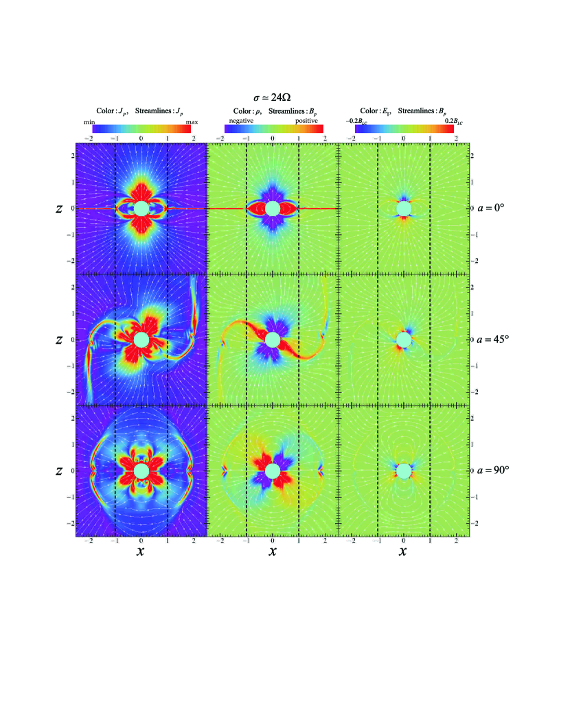
Figure 3: The non-Ideal magnetospheric solutions in the poloidal plane $(\boldsymbol{\mu},\mathbf{\Omega})$ for prescription (B) and for a high $\sigma$ value ($\sigma=24\Omega$). Each row shows the solutions corresponding to the indicated inclination angles $a$. The left-hand column shows the poloidal current modulus (in color scale) together with the streamlines of the poloidal current. The middle column shows the charge density (in color scale) together with the field lines of the poloidal magnetic field. The color ranges purple-green and green-red indicate negative and positive charge density, respectively. The right-hand column shows the parallel electric field component $E_{\parallel}$ (in color scale) together with the lines of the poloidal magnetic field. The color ranges purple-green and green-red indicate antiparallel and parallel directions of $E_{\parallel}$ (relative to the magnetic field) respectively. Note that the color representation for $E_{\parallel}$ saturates beyond the absolute value $0.2B_{LC}/c$ where $B_{LC}$ is the value of the stellar magnetic dipole field at the distance $R_{\text{LC}}$. The structure shown in the first two columns is quite similar to that of the FFE solutions (the main difference from the FFE solution can be seen in the third column).

In Fig. 3 we present the magnetospheric structures that we obtain on the poloidal plane $(\boldsymbol{\mu},\mathbf{\Omega})$ using prescription (B) for $\sigma\simeq 24\Omega$. Each row corresponds to the structure at a different inclination angle $a=(0^{\circ},45^{\circ},90^{\circ})$ as indicated in the figure. The first column shows the modulus of the poloidal current $J_{p}$ in color scale together with its streamlines. The second and third columns show, in color scale, the charge density $\rho$ and $E_{\parallel}$ respectively, together with the streamlines of the poloidal magnetic field $\mathbf{B_{p}}$. We observe that for this high $\sigma$ value the global structures are similar to those of the FFE solutions (see Contopoulos & Kalapotharakos, 2010). Even for the $a=0^{\circ}$ case that has the most different value of the Poynting flux from that of the FFE solution, the current sheet both along the equator (outside the LC) and along the separatrices (inside the LC) does survive despite the effects of non-zero resistivity. However, we do observe magnetic field lines reconnecting gradually on the equatorial current sheet beyond the LC. The main differences between these solutions and the FFE ones are highlighted in the third column where we plot the parallel electric field $E_{\parallel}$ developed during the evolution of the simulation. For $a=0^{\circ}$ there is a significant parallel electric field component along the separatrices as well as over the polar caps. The direction of the $\mathbf{E_{\parallel}}$ follows the direction of the current $\mathbf{J}$. Thus, $\mathbf{E_{\parallel}}$ within the return current region (the separatrices and a small part of the polar cap near them) points outward while in the rest of the polar cap region points inward. There is also a weaker parallel component ${\bf E}_{||}$ along the equatorial current sheet (not clearly shown in the color scale employed). As $a$ increases, the inward pointing $\mathbf{E_{\parallel}}$ component in the central part of the polar cap becomes gradually offset. During this topological transformation the branch of the polar cap area corresponding to the return current becomes narrower while the other one becomes wider. At $a=90^{\circ}$, $\mathbf{E_{\parallel}}$ is directed inwards in half of the polar cap and outwards in the other half. This topological behavior is similar to that of the poloidal current in the FFE solutions. For $a\neq 0^{o}$ there is a clearly visible component of $\mathbf{E_{\parallel}}$ in the closed field lines area as well as along the equatorial current sheet outside the LC.

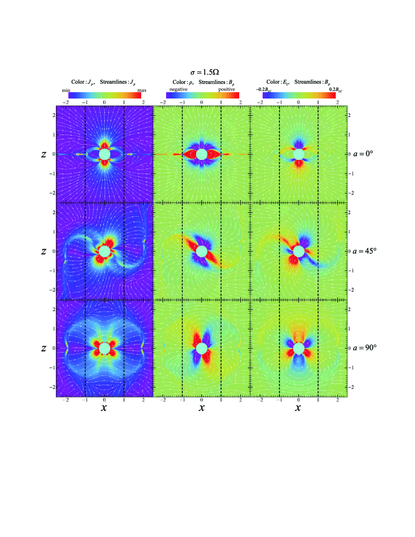
Figure 4: Similar to Fig. 3 but for a much lower $\sigma$ value ($\sigma=1.5\Omega$). The main magnetospheric features such as separatrices and current sheets can still be observed, even though they now appear much weaker. The magnetic field lines close well beyond the LC and the parallel electric field components reach higher values than those of Fig. 3

Figure 4 shows the same plots as Fig. 3 and in the same color scale but for $\sigma\simeq 1.5\Omega$. Although the non-Ideal effects have been amplified, the global topological structure of the magnetosphere has not changed dramatically. We can still distinguish traces of the current sheet even in the $a=0^{\circ}$ case, whose Poynting flux is substantially reduced from that of the FFE case. As noted above, the magnetic field lines close now beyond the LC, due to the finite resistivity that allows them to slip through the outflowing plasma. The parallel electric field component $\mathbf{E_{\parallel}}$ is non-zero in the same regions as those seen in the higher $\sigma-$values; its topology also is not very different from that of these cases, but its maximum value increases with decreasing $\sigma$. We note also that despite the fact that the dissipative energy losses corresponding to the various values of $a$ are quite different (see Fig. 2a), the corresponding maximum values of $E_{\parallel}$ are quite similar.

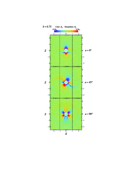
Figure 5: Similar to the third columns of Figs. 3, 4 but for the prescription (A) and for the $b=0.75$ value. For this value of $b$ the corresponding $L$ values are the same to those of the simulations presented in Fig. 4. The structure of these solutions seems very similar (qualitatively) to those of Fig. 4.

We have also run many simulations implementing prescription (A) for various values of the fraction $b$ of the non-zero parallel electric field component $E_{\parallel}$. We have covered this way the entire spectrum of solutions from the vacuum to the FFE one. The ensemble of solutions that connects these two limits seems to be similar to that of prescription (B). It seems that there are pairs of the values of the fraction $b$ and the conductivity $\sigma$ that lead to very similar (qualitatively) solutions. In Fig. 5 we plot the poloidal magnetic field lines together with the parallel electric field component $E_{\parallel}$ in color scale (similar to the third column of Figs. 3 and 4) for $b=0.75$ which has the same Poynting flux with the simulation of prescription (B) with $\sigma=1.5\Omega$. We see that the magnetospheric structures of the two solutions are quite close (compare Fig. 5 with the third column of Fig. 4). Also, our results are qualitatively very similar to those of Li et al. (2011) who, as noted, implemented a much more elaborate prescription for $\mathbf{J}$ based on Ohm’s law.

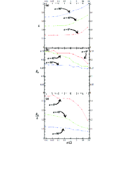
Figure 6: Similar to Fig. 2 but for prescription (C) - SFE. This prescription does not cover the entire spectrum of solutions between the vacuum and FFE ones since for $\sigma\rightarrow 0$ we still get a dissipative configuration rather than the vacuum solution. However, as $\sigma\rightarrow\infty$, the corresponding Poynting flux values tend to those of the FFE solutions. The dissipative energy loss rate $\dot{E}_{D}$ exhibits a maximum value for $\sigma\rightarrow 0$ and remains non-zero even for the high $\sigma$ values due to the persistent dissipation on the current layer outside the LC. This result seems to confirm Gruzinov who argued that the SFE solutions for $\sigma\rightarrow\infty$ present finite dissipation on the current layer.

Figure 6 is similar to Fig. 2 but for prescription (C) - i.e. SFE, assuming the value of $\sigma$ to be constant. This prescription does not tend to the vacuum solution for $\sigma=0$ but to a special solution with $J/\rho c=1$. As in Fig.2 all quantities presented in this figure correspond to average values over 1 stellar period ($4^{\text{th}}$ rotation). The Poynting flux behaves accordingly, relaxing to $L\simeq 0.55\mu^{2}\Omega^{4}/c^{3}$ for $a=0^{\circ}$ (rather than zero), $L\simeq 1.0\mu^{2}\Omega^{4}/c^{3}$ for $a=45^{\circ}$ and $L\simeq 1.4\mu^{2}\Omega^{4}/c^{3}$ for $a=90^{\circ}$ as $\sigma\rightarrow 0$. These values are 55%, 65% and 70% of the corresponding FFE values, respectively. For high $\sigma$ values ($\sigma\rightarrow\infty$) the corresponding solutions have a Poynting flux close to that of the FFE solutions.

The dissipation power in this case is given by

$$\begin{split}\dot{E}_{D}&=\int_{r_{1}<r<r_{2}}\mathbf{J}\cdot\mathbf{E}\ {\rm d}V\\ &=\int_{r_{1}<r<r_{2}}E_{0}\sqrt{\rho^{2}c^{2}+\gamma^{2}\sigma^{2}E_{0}^{2}}\ {\rm d}V\end{split}$$ (11)

and, as expected, is non-zero even for $\sigma=0$. For $\sigma=0$ we get the highest value for $\dot{E}_{D}$, either in absolute sense or as a fraction of the Poynting flux. These reach 45%, 25% and 12% for $a=0^{\circ},a=45^{\circ},a=90^{\circ}$ respectively. These are higher than the highest values we got using prescription (B). Their increased magnitude is mostly due to the increase in the $\dot{E}_{D}$ of the SFE solutions on the current sheet outside the LC. We observe also that the dissipation remains at high levels even for very high values of the conductivity and only the $a=0^{\circ}$ case (which is the most dissipative one) shows a clear tendency of decreasing $\dot{E}_{D}$ with $\sigma$. For $\sigma\gg 1$ the dissipation energy inside the LC decreases significantly while it remains almost constant outside the LC. We have tried higher resolution simulations that allow higher values of $\sigma$ without any apparent decrease of the dissipation on the current sheet. This appears to confirm Gruzinov’s claim that SFE allows for non-zero dissipation on the current sheet even for $\sigma\rightarrow\infty$.

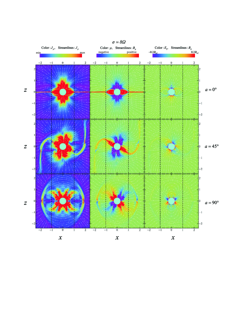
Figure 7: Similar to Figs. 2, 3 but for prescription (C) - SFE and for a high $\sigma$ value ($\sigma=8\Omega$). The Poynting flux of these solutions tend to those of the FFE ones. Nevertheless, we still see magnetic field lines closing well outside the LC (especially for $a=0^{\circ}$). The electric current in the SFE prescription is everywhere space-like ($J/\rho c>1$). However, there are regions that are effectively time-like (as defined in the text). These are the noisy regions in the polar cap vicinity (for $a\neq 90^{\circ}$) seen in the third column. Their noisy character is due to the continuously changing direction of the electric field.

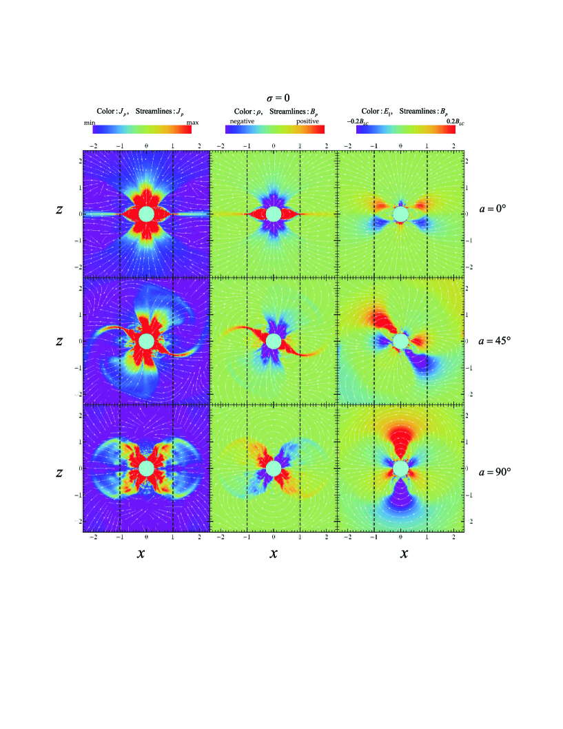
Figure 8: Similar to Fig. 7 but for $\sigma=0$ value. The modulus of the parallel electric field components increases along with the area of their influence. The closed field line regions of the oblique rotators show significant parallel electric field components; however, the dissipation there is insignificant because the value of the product $\mathbf{J}\cdot\mathbf{E}$ is small.

Figure 7 depicts the same quantities as Figs. 3, 4 but for prescription (C) i.e. SFE and for $\sigma\simeq 8\Omega$. We observe that the magnetospheric structures in this case are very close to those of FFE (especially for $a>0^{\circ}$). The magnetic field lines open not much farther than the LC and the usual equatorial current sheet develops beyond that. In the third column, which shows the parallel electric field, we see that in the effectively time-like regions near the star the color is “noisy” as a result of the constant change of its sign during the evolution. In the next section we are going to discuss possible implications of these types of behavior in these regions. The regions with the “calm” (non noisy) electric fields correspond to space-like currents. We discern these electric fields mostly along the separatrix in the aligned rotator and along the undulating equatorial current sheet in the non-aligned rotator. We note that for $a=90^{\circ}$ the entire polar cap region consists of such components. In Fig. 8 we present the results for the same prescription, i.e. (C) - SFE, but for $\sigma=0$. As we have mentioned in §2, these cases are significantly different from the vacuum solution. The magnetic field lines close well outside the LC while we are able to discern traces of the equatorial current sheet. We observe again the “noisy” regions near the star (this is the way that SFE deals with time-like currents, namely as fluctuating space-like ones). In the axisymmetric case ($a=0^{\circ}$) we see that the value of $E_{\parallel}$ as well as the area over which it occurs increase for the smaller values of $\sigma$. For $a>0^{\circ}$ the value that $E_{\parallel}$ reaches near the polar cap is not significantly higher that that of Fig. 7. However, the new interesting feature in the oblique rotators is the development of high $E_{\parallel}$ in specific regions of the closed field lines areas. These configurations do not imply high dissipation since the corresponding currents are very weak there.

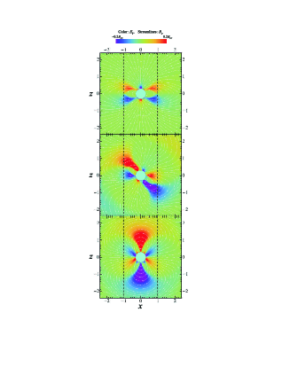
Figure 9: The third column of Fig. 8 considering the average values of the fields within a stellar period. The “noisy” behavior shown in Fig. 8 is now disappeared. These regions reveal their effectively time-like behavior.

In order to reveal the on-average behavior of the effectively time-like regions we considered the average values of the fields within one stellar period. In Fig. 9 we plot for the SFE ($\sigma=0$) the corresponding (average) parallel electric components $\overline{E_{\parallel}}$ together with the magnetic field lines (similar to the third columns in Figs. 7 and 8). We see that the “noisy” behavior has disappeared. As we discussed previously one can imagine the existence of hybrid solutions (e.g. non “noisy” behavior in the closed field line regions like that shown in Fig. 9) and a “noisy” one in the open field line regions like that shown in Fig. 7.

Finally, we note that for all the solutions presented in this section, the regions corresponding to high values of $\mathbf{J}\cdot\mathbf{E}$ are traced mostly by the high values of $J$ (e.g. near the current layers). However, as we observe in Figs. 3-4, 7-8 there are regions corresponding to high values of $E_{\parallel}$ that do not lie near the current sheet. This implies that high energy particles supporting the pulsar emission may be generated not near the regions of high $\dot{E}_{D}$ but near those with high values of $E_{\parallel}$ .

4 Solutions with $J=\rho c$

As argued above, the time evolution of the MHD equations requires a prescription that relates the current density $\mathbf{J}$ and the fields, given above by the different forms of Ohm’s law. However, given that any value of ${\bf E_{\parallel}}$ appropriate for pulsars would quickly accelerate any charges to velocities close to $c$, it would be reasonable to assume that the relation $J\simeq\rho c$ will be attained between the current and charge densities. Motivated by these considerations, rather than determine the current $\mathbf{J}$ from its relation to $\mathbf{E_{\parallel}}$, we determine it from its relation to the local charge density $\rho$. Specifically, we focus our attention to solutions with $J/\rho c=1$. This specific ratio is special because it discriminates between magnetospheres consistent with only a single sign charge carrier ($J/\rho c\mathrel{\raise 1.29167pt\hbox{$<$}\mkern-14.0mu\lower 2.58334pt\hbox{$\sim$}}1$) and those that require carriers of both signs of charges ($J/\rho c>1$) to ensure the counter streaming required in space-like current flows. Since each flow line with $J/\rho c>1$ requires at some point a source of charges of the opposite sign, it is considered that such flows by necessity involve the production of pairs and their associated cascades.

One well-studied location for charge production in the pulsar magnetosphere is the polar cap, where particle acceleration and pair cascades are thought to take place. If charges of either sign are freely supplied by the neutron star surface, as is thought to be the case in all but magnetar-strength fields (Medin & Lai, 2010), then a maximum current of $J/\rho c=1$ can flow outward above the polar cap in Space-Charge Limited Flow (SCLF). In this case, an accelerating electric field $E_{\parallel}$ is produced by a charge deficit $\Delta\rho=(\rho-\rho_{GJ})$ that develops because the GJ density is different from the actual charge flow along the field lines (Arons & Scharlemann, 1979). This electric field then supports a current of primary electrons that radiates $\gamma$-rays, initiating pair cascades. The pairs efficiently screen the $E_{\parallel}$ above a pair formation front (PFF), by downward acceleration of positrons. This charge density excess is small relative to the total charge, i.e. $\Delta\rho/\rho=\epsilon\ll 1$ and the current that flows into the magnetosphere above the PFF has $J/\rho c\simeq 1$ (Harding & Muslimov, 2001). Therefore the steady-state SCLF acceleration models are only compatible with a small range ($J/\rho c\simeq 1$) of the current to charge density ratio. Beloborodov (2008) demonstrated that no discharge occurs if $J/\rho c<1$ and that the $E_{\parallel}$ and the discharge generated when $J/\rho c>1$ or $J/\rho c<0$ (implying that the current direction is opposite to the one that corresponds to outward movement of the Goldreich-Julian charges) are strongly time dependent. This has been confirmed by models of time-dependent SCLF pair cascades (Timokhin & Arons, 2011).

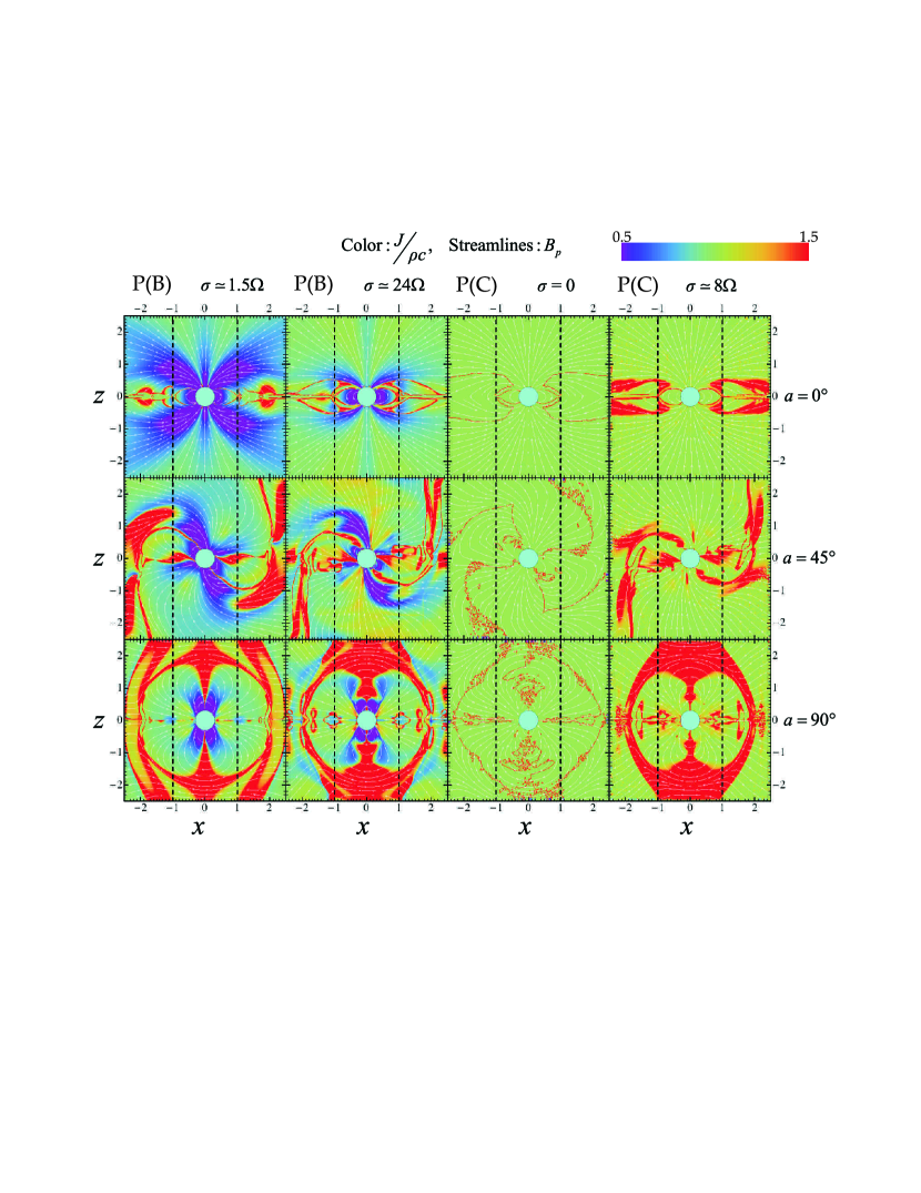
Figure 10: The ratio $J/\rho c$ (in color scale) together with the poloidal magnetic field lines for the solutions presented in Figs. 3, 4, 7, 8 as indicated in the Figure. The ratio $J/\rho c$ in prescription (B) decreases in general as $\sigma$ decreases and goes towards 0 for $\sigma\rightarrow 0$. In prescription (C) - SFE the ratio $J/\rho c$ goes to 1 (null current) as $\sigma\rightarrow 0$ while it is higher than 1 for $\sigma>0$. However, in both these cases there are regions where the current has on average time-like ($J/\rho c<1$) behavior (effectively time-like; see Fig. 9).

With this emphasis on the ratio $J/\rho c=1$, we show in Figure 10 the values of $J/\rho c$ in color scale together with the magnetic field lines on the poloidal plane for the parameters of the simulations of prescription (B) given earlier in Figs. 3-4 and prescription (C) given in Figs. 7-8. These plots can be directly compared to the FFE magnetosphere of Fig. 1.

The first two columns of Fig. 10 indicate that as $\sigma$ in prescription (B) ranges from large values ($\sigma=24\Omega$; the FFE has strictly speaking $\sigma=\infty$) to 0 (vacuum) the ratio $J/\rho c$ decreases tending to 0 for $\sigma\rightarrow 0$. This can be seen by inspection of Eq. (5), the first term of which corresponds always to a time-like current, with a space-like current arising only through the effects of the second term. Hence there must be some spatial distribution of $\sigma$ values below which no space-like region exists because the $\sigma E_{\parallel}$ term is small enough.

The next two columns of Fig. 10, showing the $J/\rho c$ ratio of Prescription (C) - SFE, are interesting because this prescription leads to $J/\rho c=1$ for $\sigma\rightarrow 0$, while tending near the FFE values for $\sigma\rightarrow\infty$, but only in the space-like current regions of the FFE solutions. The time-like current regions of the FFE solutions are now only “effectively time-like”, as discussed by Gruzinov, resulting in the “fluctuating” or “noisy” behavior that is apparent there.

Suspecting that the “fluctuating” (or “noisy”) behavior of the effectively time-like current regions of SFE is due to the imposed relation between $J$ and $\rho c$, we modified prescription (B) to search for local values of $\sigma$ that would be consistent with $J/\rho c=1$. More specifically, we consider a $\sigma$ variable in time and space so that the total $J$ provided by Eq. (5) is everywhere and at every time step, equal to $\rho c$. However, we found that there are regions where $E_{\parallel}$ goes to zero for a current $J$ less than $\rho c$. In these regions the second term in the expression for $J$, namely $\sigma E_{\parallel}$, tends to the second term of the FFE current expression (Eq. 3) being unable to comply with the $J=\rho c$ constraint. These regions demand extremely high values of $\sigma$ in order to achieve the $J/\rho c=1$ relation due to the vanishing $E_{\parallel}$ values. We have dealt with this numerically by setting a maximum value of $\sigma$ ($=50\Omega$) that provided a realistic suppression of the $E_{\parallel}$ in these regions.

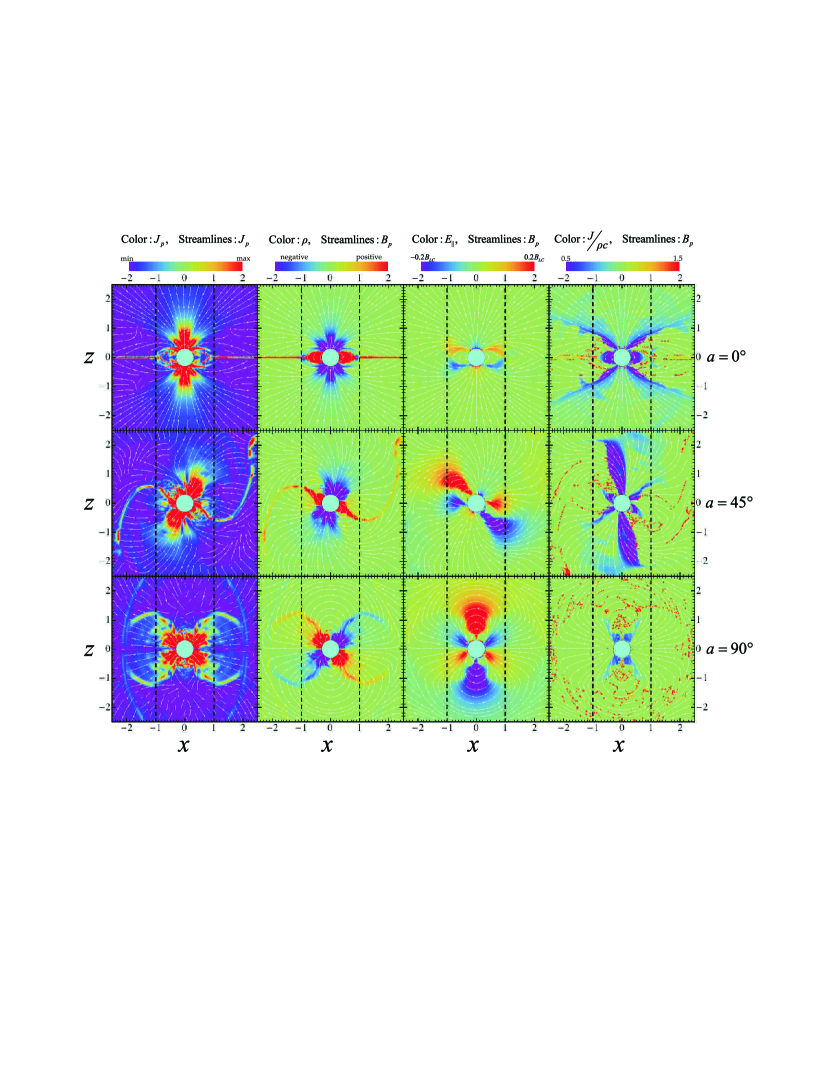
Figure 11: The solutions employing prescription (B) with the $\sigma-$values adapted locally to achieve $J/\rho c$ as close to 1 as possible. The first three columns are similar to those of Figs. 3, 4, 7, 8 while the fourth column shows the corresponding ratio $J/\rho c$ in color scale. The main features (e.g. current sheets, separatrices) of the FFE solutions are still discernible. We observe parallel electric field components across the polar caps and along the separatrices. For the oblique rotators parallel electric field components exist also in parts of the closed field line regions. However, the latter regions show low dissipation energy rate $\dot{E}_{D}$ since the corresponding product $\mathbf{J}\cdot\mathbf{E}$ is small. In the fourth column we observe regions with $J/\rho c<1$. In these regions a current density $J$ smaller than the value $\rho c$ is enough so that the corresponding parallel electric field component vanishes. This kind of solutions are the upper limit of the solutions that can be considered that are supported by charge separated flows.

Figure 11 shows the results of such an approach. The first three columns provide respectively the values of the poloidal current $J_{p}$, charge density $\rho$ and parallel electric component $E_{\parallel}$ and are similar to those presented in Figs. 3, 4, 7, 8, while the fourth column shows the values of the $J/\rho c$ ratio in color scale together with the poloidal magnetic field lines. The corresponding $L$ and $\dot{E}_{D}$ values as well as their ratios $\dot{E}_{D}/L$ have been denoted in Fig. 2 by the horizontal dashed lines. Not surprisingly, these solutions are similar to those of prescription (C) - SFE in the $\sigma\rightarrow 0$ regime (see Fig. 8). The essential difference between these two approaches is that, in distinction with SFE, this approach can handle time-like currents without the need - like SFE - to do so only on average (see blue and purple color regions in the fourth column).

To allow our solutions even larger flexibility in attaining $J=\rho c$ we have looked for prescriptions that divorce $\mathbf{J}$ from ${\bf E_{\parallel}}$, replacing the second term of Eq. (5), with a term of the form

$$\mathbf{J_{\parallel}}=f\;\mathbf{B},$$ (12)

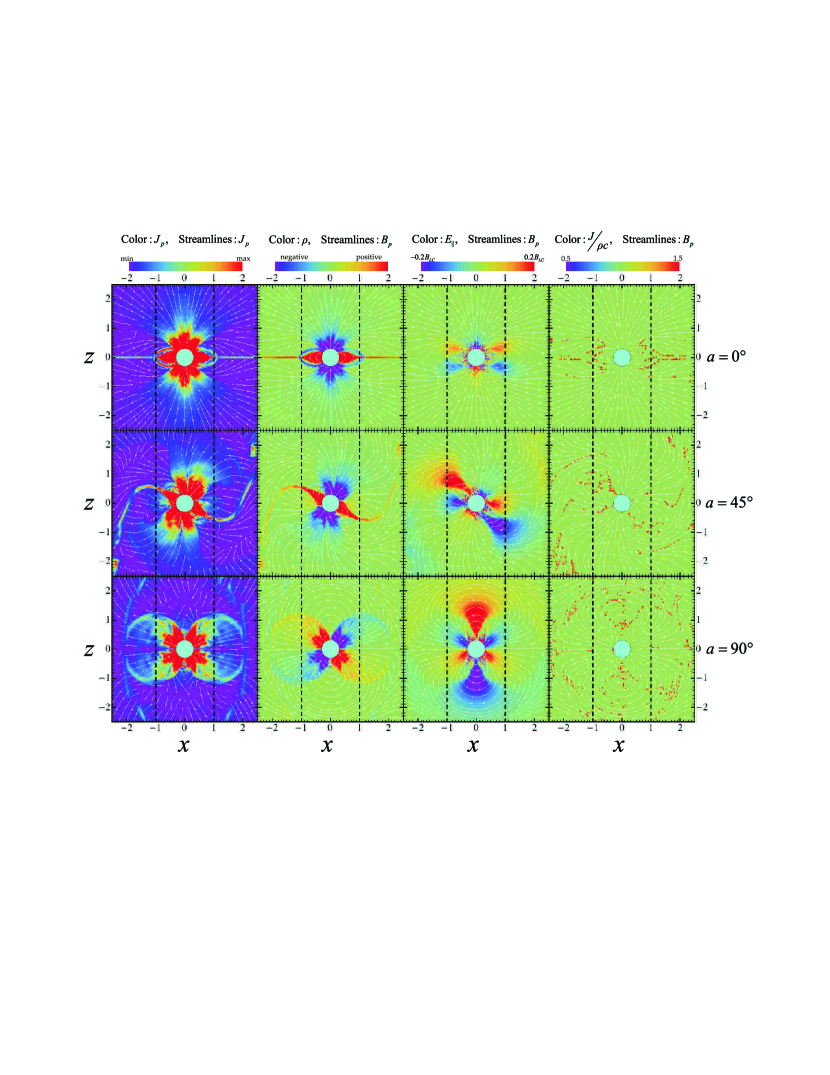
Figure 12: Similar to Fig. 11 but with the parallel current density independent of the modulus of ${\bf E_{\parallel}}$ (see Eq. 12). As shown in the fourth column, this prescription achieves $J/\rho c=1$ in the entire magnetosphere. This leads to an oscillating behavior for ${\bf E_{\parallel}}$ in the time-like current regions of the simulation presented in Fig. 11, similar to that of SFE (Fig. 8). We note that this effect is more general and appears wherever the ratio $J/\rho c$ is enforced to have values above those that are sufficient to cancel out the parallel electric component. This behavior is the result of the mutual response between the electric field and the current density and may be crucial for the coherent radio emission.

where $f$ is a scalar quantity having a local value that ensures the local value of the ratio $J/\rho c$ to be equal to 1. The difference from the previous approach and that of prescription (B) is that this term is not related anymore to the value of $E_{\parallel}$, other than that it is directed along (or against for $f<0$) the direction of the magnetic field. The sign of $f$ is determined so that the direction of $\mathbf{J_{\parallel}}$ coincides with that of $\mathbf{E_{\parallel}}$. The results of these simulations are shown in Fig. 12 the panels of which are similar to those of Fig. 11. The global structure in this case is very similar to that of the simulation presented in Fig. 11 except for the time-like regions (especially those near the star) that now exhibit the “noisy” behavior of the SFE simulations. However, the ratio $J/\rho c$ is now everywhere equal to 1. Our solution has therefore the required property ($J/\rho c=1$) at the expense of producing a “noisy” behavior indicative of time variations at these limited spatial scales.

This oscillatory behavior (both here and in the SFE cases) is a rather generic feature that occurs in the time-like current regions for values of $J/\rho c$ larger than those needed to “kill” the local $\mathbf{E}_{\parallel}$ implied by the field evolution equations; both within the prescription of Eq. (12) and within SFE, at these higher values, $J$ and $E_{\parallel}$ end up pointing in different directions and an oscillatory behavior ensues. Smaller values of $J/\rho c$, cannot drive ${\bf E_{\parallel}}$ to zero and allow the magnetosphere to attain steady state, leaving a non-oscillatory component of $\mathbf{E}_{\parallel}$ along the direction of $\mathbf{J_{\parallel}}$. Viewed this way, the ideal condition ${\bf E\cdot B=0}$ is one that requires a local delicate balance between its parameters (e.g. $J,\rho$). If, for whatever reason or necessity, this balance breaks, the magnetosphere develops locally an oscillatory behavior. The robustness and the true evolution of this behavior will be determined by the microphysical plasma properties as they mesh within the global framework of the magnetosphere electrodynamics.

The conclusion of this exercise is that solutions with a specific value of $J$, for example $J=\rho c$ everywhere, can be implemented with a sufficiently general expression for $\mathbf{J_{\parallel}}$, provided that one is willing to accept locally time varying solutions.

Note that in this prescription, as well as in SFE, the current is forced to follow the relation $J=\rho c$ or $J>\rho c$ (for $\sigma\neq 0$ in SFE) even in the closed field line regions producing even there this “noisy” (fluctuating) behavior. Although applying this $J-\rho$ prescription there is not forbidden a priori, it would be reasonable to consider that this condition is actually not valid in the closed field lines and that a different condition should be used there. However, the implementation of a different prescription for these regions remains cumbersome because it demands that we determine whether the magnetic field lines at each grid point are actually open or closed and then apply for them this different condition. Nevertheless, even if we were to enforce a prescription that removes the fluctuating (noisy) behavior in the closed field line regions, this should not affect the similar behavior on the open field line regions.

5 Discussion and Conclusions

Up to now, the pulsar radiation problem has been studied considering either the vacuum (Deutsch, 1955) or the FFE solutions (Contopoulos et al., 1999; Spitkovsky, 2006; Kalapotharakos & Contopoulos, 2009) for the structure of the underlying magnetosphere. The vacuum solutions have analytical expressions while the FFE solutions have only been studied numerically in the last decade. However, neither solution is compatible with the observed radiation; the former because it is devoid of particles and the latter because it precludes the presence of any ${\bf E_{\parallel}}$. The physically acceptable solutions have to lie somewhere in the middle. As of now, there are no known solutions that incorporate self-consistently the global magnetospheric structure along with the microphysics of particle acceleration and radiation emission. The goal of the present work has been to explore the properties of pulsar magnetospheres under a variety of prescriptions for the macroscopic properties of the underlying microphysics in anticipation of a more detailed future treatment of these processes. It should be noted that these processes lie outside the purview of the equations used to evolve the electric and magnetic fields. Nonetheless, for most models examined the dissipation power does not exceed 10-20% of the spin-down one; this value is consistent with the observed radiative efficiencies of the millisecond pulsars (Abdo et al., 2009a), that are the ones reaching the highest efficiencies of all pulsars, suggesting that energetically, realistic magnetospheres may be well approximated by our models.

In order to explore the non-Ideal ${\bf E\cdot B\neq 0}$ regime we considered several prescriptions discussed in §3, 4 and analyzed their properties in detail (Figures 2 - 9). Despite their intrinsic interest, the solutions discussed above still need to be examined more closely for consistency with the microphysics responsible for the set up and closure of the corresponding magnetospheric circuits, which are characterized by a considerable range in the distribution of the ratio $J/\rho c$. On the other hand, there are studies arguing that it is essential that the ratio $J/\rho c$ be near 1 in order for steady-state pair cascades to be generated near the polar cap. Besides that, solutions corresponding to values $J/\rho c<1$ can be considered as the range of configurations without pair production, since such solutions can be supported by charge separated flows.

With the value $J/\rho c=1$ given this particular significance, we have pursued a search for solutions that are driven by adherence to this condition in as broad a spatial range as possible. As noted in the previous section we did so by searching for solutions of variable conductivity $\sigma$, or by employing expressions for the parallel current unconstrained by the values of the parallel electric field. We found that arbitrary values of $\sigma$, while allowing $J/\rho c=1$ in most areas, in certain others can drive $\mathbf{E}_{\parallel}$ to zero sufficiently fast to restrict $J$ to values $J<\rho c$. As noted in the previous section, a more general expression for $J$ not related to $\mathbf{E}_{\parallel}$ can produce $J/\rho c=1$ everywhere but only at the expense of fluctuations in regions where the value of $J/\rho c$ is larger than that necessary to null the local $\mathbf{E}_{\parallel}$ implied by the field evolution equations. These results indicate the importance of the value of the ratio $J/\rho c$ vis-á-vis the presence of pair cascades and steady-state emission in pulsar magnetospheres.

The actual behavior of the magnetosphere is likely to be more complicated than that described by the current density prescriptions provided in this work (Eqs. 5, 6 and 12). Physics beyond those of the magnetic and electric field evolution equations will introduce novel time scales that will determine the response of the current density to the parallel electric field component and vice versa. The implications of such an oscillatory behavior which involves an electric field that alternates direction, may in fact provide an account of the pulsar coherent radio emission, as such a behavior is the essential ingredient of cyclotron maser emission (Melrose, 1978; Levinson et al., 2005; Melrose, 2006; Luo & Melrose, 2008). To the best of our knowledge, the above argument is the first ever to suggest a relation between the global properties of pulsar magnetospheres and their coherent radio emission.

These more general models of non-ideal magnetospheres discussed above are possibly related to the behavior and properties of intermittent pulsars, which may, if more of them are discovered, provide meaningful constraints on their radiation mechanism and magnetospheric dynamics. Intermittent pulsars are pulsars found in “on” and “off” radio states (Lyne, 2009). The interesting aspect of these objects is that they exhibit different spin-down rates in their “on” and “off” states; even more interesting is the fact that they apparently “remember” the spin-down rate they had in the previous cycle, as they return to the same spin-down rate when switching from “on” to “off” and vice versa. The ratios of the “on” to “off” spin-down rates are 1.5 – 1.7 for pulsars PSR B1931+24 (Kramer et al., 2006) and PSR J1832+0029 (Lorimer et al., 2006; Lyne, 2009), while it is 2.5 for the more recently observed PSR J1841-0500 (Camilo et al., 2012). Interestingly these values are well below the minimum ratio 3 between the FFE and the vacuum spin-down rates. Based on this observation, Li et al. (2011) argued that the “on” state can be the FFE solution while the “off” state simply a resistive solution corresponding to a certain value of $\sigma$.

An alternative view is to identify the “on” state with magnetosperes with $J/\rho c>1$ and the “off” one with those of $J/\rho c<1$, given the necessity of the presence of pairs (accompanied by the radio emission) in the former and their likely absence (and also of radiation) in the latter. In fact, the ratio of spin-down rates between the FFE and the $J/\rho c=1^{-}$ magnetospheres is within $1.4-1.8$ (see Figs. 2 and 6), with the higher values corresponding to the lower values of $a$. This would be consistent with the observations of the first two intermittent pulsars. However, this is not consistent with the spin-down ratio of the third intermittent pulsar whose “on” and “off” states may be magnetospheres with different values of $\sigma$. The discovery of a larger sample of intermittent pulsars (especially if one could also put some limits on their inclination angles) would be extremely useful in constraining magnetospheric models. For example if the ratio of the “on/off” spin-down rate was found not to exceed the value 3, one would have to exclude the vacuum solution being the “off” state, since for sufficiently small $a$ this ratio becomes arbitrarily large.

The solutions we presented in this work, besides their intrinsic interest, can serve to produce model pulsar $\gamma-$ray light curves in a way similar to that of Contopoulos & Kalapotharakos (2010); Bai & Spitkovsky (2010a); Venter et al. (2009); Harding et al. (2011). Such models will provide a means of connecting the structure and physics of magnetospheres to observations, since they constrain the pulsar magnetospheric geometry as well as the regions of anticipated particle acceleration and even the values of the accelerating electric fields. These will therefore provide independent tests of these models for real pulsars.

The next level of this study should include microphysics at a level sufficient to allow some feedback on the global solutions i.e. the production of pairs whose effects are included in the computation of the local $E_{\parallel}$ self–consistently. It will be of interest to examine whether such solutions are consistent with the charge separated flows or whether they require an inherently time dependent magnetosphere, a feature that could be tested observationally. The time dependence should lead to oscillations of the pulsar emission with frequency of order $\nu\mathrel{\raise 2.15277pt\hbox{$>$}\mkern-14.0mu\lower 2.58334pt\hbox{$\sim$}}\Omega/2\pi$ for emission near the LC and $\nu\gg\Omega/2\pi$ for emission near the polar cap. We have searched and found not these oscillations in the X-ray domain of several pulsar light curves. Either they were not present at the objects we searched or they lose their coherence at these much lower energies. Nonetheless, we intend to study the possibility of the presence of such oscillation in a future work.

Figure 2: (a) The Poynting fluxes $L$ (measured on the surface of the star) as a function of $\sigma$ in log-linear scale for prescription (B). Red, green and blue colors correspond to $a=0^{\circ}$ (aligned), $a=45^{\circ}$ and $a=90^{\circ}$ perpendicular rotator, respectively. The horizontal solid line elements denote the $L$ values corresponding to the vacuum (lower value) and the FFE (higher value) solutions. Note that the $L$ value for $a=0^{\circ}$ is similar to the vacuum one for $\sigma\lesssim 0.3\Omega$ ($\Omega$ is the angular frequency of the star) and it reaches that of the FFE solution only for much higher $\sigma$ values; (b) The dissipation energy rate $\dot{E}_{D}$ integrated over the volume bounded by radii $r_{1}=r_{\star}=0.3R_{\text{LC}}$ and $r_{2}=2.5R_{\text{LC}}$ as a function of $\sigma$; (c) The fraction $\dot{E}_{D}/L$ never exceeds the values 10%-20%, while for $\sigma\rightarrow 0$ and $\sigma\rightarrow\infty$ it goes towards 0. The dashed horizontal lines in all three panels denote the values corresponding to simulations with $J/\rho c=1$ (see §4, 5).

References

- Abdo et al. (2009a) Abdo, A. A., et al. 2009a, Science, 325, 848
- Abdo et al. (2009b) —. 2009b, ApJ, 696, 1084
- Arons & Scharlemann (1979) Arons, J., & Scharlemann, E. T. 1979, ApJ, 231, 854
- Bai & Spitkovsky (2010a) Bai, X.-N., & Spitkovsky, A. 2010a, ApJ, 715, 1282
- Bai & Spitkovsky (2010b) —. 2010b, ApJ, 715, 1270
- Beloborodov (2008) Beloborodov, A. M. 2008, ApJL, 683, L41
- Bogovalov (1999) Bogovalov, S. V. 1999, A&A, 349, 1017
- Camilo et al. (2012) Camilo, F., Ransom, S. M., Chatterjee, S., Johnston, S., & Demorest, P. 2012, ApJ, 746, 63
- Contopoulos & Kalapotharakos (2010) Contopoulos, I., & Kalapotharakos, C. 2010, MNRAS, 404, 767
- Contopoulos et al. (1999) Contopoulos, I., Kazanas, D., & Fendt, C. 1999, ApJ, 511, 351
- Daugherty & Harding (1996) Daugherty, J. K., & Harding, A. K. 1996, ApJ, 458, 278
- Deutsch (1955) Deutsch, A. J. 1955, Annales d’Astrophysique, 18, 1
- Goldreich & Julian (1969) Goldreich, P., & Julian, W. H. 1969, ApJ, 157, 869
- Gruzinov (1999) Gruzinov, A. 1999, ArXiv Astrophysics e-prints, astro-ph/9902288
- Gruzinov (2005) —. 2005, Physical Review Letters, 94, 021101
- Gruzinov (2007) —. 2007, ArXiv e-prints, 2007arXiv0710.1875G
- Gruzinov (2008) —. 2008, ArXiv e-prints, 2008arXiv0802.1716G
- Gruzinov (2011) —. 2011, ArXiv e-prints, 2011arXiv1101.3100G
- Harding et al. (2011) Harding, A. K., DeCesar, M. E., Miller, M. C., Kalapotharakos, C., & Contopoulos, I. 2011, ArXiv e-prints 1111.0828
- Harding & Muslimov (2001) Harding, A. K., & Muslimov, A. G. 2001, ApJ, 556, 987
- Harding et al. (2008) Harding, A. K., Stern, J. V., Dyks, J., & Frackowiak, M. 2008, ApJ, 680, 1378
- Kalapotharakos & Contopoulos (2009) Kalapotharakos, C., & Contopoulos, I. 2009, A&A, 496, 495
- Kalapotharakos et al. (2011) Kalapotharakos, C., Contopoulos, I., & Kazanas, D. 2011, MNRAS (in press)
- Komissarov (2006) Komissarov, S. S. 2006, MNRAS, 367, 19
- Kramer et al. (2006) Kramer, M., Lyne, A. G., O’Brien, J. T., Jordan, C. A., & Lorimer, D. R. 2006, Science, 312, 549
- Levinson et al. (2005) Levinson, A., Melrose, D., Judge, A., & Luo, Q. 2005, ApJ, 631, 456
- Li et al. (2011) Li, J., Spitkovsky, A., & Tchekhovskoy, A. 2011, ArXiv e-prints, 2011arXiv1107.0979L
- Lorimer et al. (2006) Lorimer, D. R., et al. 2006, MNRAS, 372, 777
- Luo & Melrose (2008) Luo, Q., & Melrose, D. 2008, MNRAS, 387, 1291
- Lyne (2009) Lyne, A. G. 2009, in Astrophysics and Space Science Library, Vol. 357, Astrophysics and Space Science Library, ed. W. Becker (Berlin Heidelberg: Springer), 67
- Lyubarsky (2008) Lyubarsky, Y. 2008, in American Institute of Physics Conference Series, Vol. 983, 40 Years of Pulsars: Millisecond Pulsars, Magnetars and More, ed. C. Bassa, Z. Wang, A. Cumming, & V. M. Kaspi, 29–37
- Lyubarsky (1996) Lyubarsky, Y. E. 1996, A&A, 311, 172
- Lyutikov (2003) Lyutikov, M. 2003, MNRAS, 346, 540
- McKinney (2006) McKinney, J. C. 2006, MNRAS, 368, L30
- Medin & Lai (2010) Medin, Z., & Lai, D. 2010, MNRAS, 406, 1379
- Meier (2004) Meier, D. L. 2004, ApJ, 605, 340
- Melrose (1978) Melrose, D. B. 1978, ApJ, 225, 557
- Melrose (2006) —. 2006, Chinese Journal of Astronomy and Astrophysics Supplement, 6, 020000
- Mestel & Shibata (1994) Mestel, L., & Shibata, S. 1994, MNRAS, 271, 621
- Michel (1982) Michel, F. C. 1982, Reviews of Modern Physics, 54, 1
- Muslimov & Harding (2004) Muslimov, A. G., & Harding, A. K. 2004, ApJ, 606, 1143
- Romani (1996) Romani, R. W. 1996, ApJ, 470, 469
- Romani & Watters (2010) Romani, R. W., & Watters, K. P. 2010, ApJ, 714, 810
- Romani & Yadigaroglu (1995) Romani, R. W., & Yadigaroglu, I.-A. 1995, ApJ, 438, 314
- Ruderman & Sutherland (1975) Ruderman, M. A., & Sutherland, P. G. 1975, ApJ, 196, 51
- Scharlemann & Wagoner (1973) Scharlemann, E. T., & Wagoner, R. V. 1973, ApJ, 182, 951
- Spitkovsky (2006) Spitkovsky, A. 2006, ApJL, 648, L51
- Takata et al. (2007) Takata, J., Chang, H.-K., & Cheng, K. S. 2007, ApJ, 656, 1044
- Timokhin (2006) Timokhin, A. N. 2006, MNRAS, 368, 1055
- Timokhin & Arons (2011) Timokhin, A. N., & Arons, J. 2011, in preparetion
- Uzdensky (2003) Uzdensky, D. A. 2003, ApJ, 598, 446
- Venter et al. (2009) Venter, C., Harding, A. K., & Guillemot, L. 2009, ApJ, 707, 800