High Velocity Precessing Jets from the Water Fountain IRAS 18286$-$0959 Revealed by VLBA Observations

Abstract

We report the results of multi-epoch VLBA observations of the 22.2 GHz H₂O maser emission associated with the “water fountain” IRAS 18286$-$0959. We suggest that this object is the second example of a highly collimated bipolar precessing outflow traced by H₂O maser emission, the other is W 43A. The detected H₂O emission peaks are distributed over a velocity range from $-50$ km s^-1 to 150 km s^-1. The spatial distribution of over 70% of the identified maser features is found to be highly collimated along a spiral jet (jet 1) extended southeast to northwest, the remaining features appear to trace another spiral jet (jet 2) with a different orientation. The two jets form a “double-helix” pattern which lies across $\sim$200 milliarcseconds. The maser distribution is reasonably fit by a model consisting of two bipolar precessing jets. The 3D velocities of jet 1 and jet 2 are derived to be 138 km s^-1 and 99 km s^-1, respectively. The precession period of jet 1 is about 56 years. For jet 2, three possible models are tested and they give different values for the kinematic parameters. We propose that the appearance of two jets is the result of a single driving source with significant proper motion.

1 Introduction

An asymptotic giant branch (AGB) star is usually spherical in shape, while a planetary nebula often exhibits a bipolar or even multi-polar morphology (Kwok 2008; 2010, and references therein). The mechanism that causes the morphological change is unclear, however it is suggested that high velocity outflows originating from AGB or post-AGB stars are closely related to the shaping of planetary nebulae (Sahai & Trauger 1998).

The term “water fountain” is used to describe a fast, collimated, molecular outflow that can be traced by H₂O maser emission (Likkel & Morris 1988). The outflow velocity is larger than the typical expansion velocity of an OH/IR star’s circumstellar envelope ($10-20$ km s^-1) revealed by 1612 MHz OH maser emission often associated with evolved stars (te Lintel Hekkert et al. 1989). From the view point of stellar evolution, this type of object is in the transition phase from an AGB star to the central star of a planetary nebula, during this phase the mass loss rate reaches its maximum. It is believed that water fountains are closely related to the shaping of planetary nebulae (Imai 2007), and the high mass-loss rate during this stage contributes significantly to the redistribution of matter from the star to interstellar space. IRAS 16342$-$3814 (Sahai et al. 1999, Claussen et al. 2009), W 43A (Diamond & Nyman 1988, Imai et al. 2002), and IRAS 19134$+$2131 (Imai et al. 2004; 2007) are representative examples of water fountain sources. IRAS 19190$+$1102 (Day et al. 2010) and IRAS 18113$-$2503 (Gómez et al. 2011) are arguably the most recent members of this class of object.

There are other discoveries with regard to water fountains besides H₂O and OH masers. The first detection of SiO maser emission associated with W 43A was reported by Nakashima & Deguchi (2003), suggesting there has been on-going, copious mass loss from the stellar surface. Imai et al. (2005) show that the distribution of the SiO maser features are well fitted by a biconically expanding model, which is not typical in AGB stars. He et al. (2008) observed the CO $J=2-1$ emission in IRAS 16342$-$3814 and Imai et al. (2009) found a very high velocity ($\sim$200 km s^-1) CO flow in CO $J=3-2$ emission from the same object. These results suggest that the high velocity outflow plays a significant role in the stellar mass loss.

The jets from water fountains are often highly collimated. Vlemmings et al. (2006) and Amiri et al. (2010) measured the magnetic field around W 43A and suggested that it plays an important role in producing the collimated jet. To date this is the only water fountain where a magnetic field has been detected associated with the jet. W 43A is also the first water fountain in which a precessing jet is observed (Imai et al. 2002; 2005). A similar jet pattern is found in an optical image of IRAS 16342$-$3814 (Sahai et al. 2005), with the authors proposing that it is a “corkscrew jet”, in which the ejecta move along a spiral path rather than having a ballistic motion as in the precessing case. However, the detailed morpho-kinematical structure of the H₂O masers in IRAS 16342$-$3814 is still unknown due to the limited number of detected H₂O maser features. Note that we define here a ballistic motion as a linear, constant velocity motion.

Other than the examples mentioned above, there is another distinctive water fountain candidate: IRAS 18286$-$0959 (hereafter abbreviated as I18286). It is one of the OH maser sources observed by Sevenster et al. (1997), and then by Imai et al. (2008). The H₂O maser emission of I18286 was first detected with the NRO 45 m telescope (Deguchi et al. 2007). Its single-dish spectrum shows many emission peaks throughout the velocity range $-50$ km s^-1 to $150$ km s^-1 with respect to the local standard of rest (LSR). The spectrum resembles the spectral profile of H₂O maser emission towards a young stellar object (YSO), nonetheless, I18286 is expected to be an AGB or a post-AGB star (see Section 5.3). Therefore, in terms of both the jet kinematics and the evolutionary status, this object has the aforementioned properties of a water fountain. The first VLBA observation of this object was undertaken shortly after its discovery (Imai 2007). Over 100 maser features were identified in a region extending more than a hundred milliarcseconds (mas).

In this paper, new VLBA results on I18286 are presented. The aim of this project is to investigate the kinematics of the high velocity component of I18286 through the motions of H₂O maser features, and to discuss the evolutionary status of this object. Details of the observations and data reduction are described in Section 2. The observational results are presented in Section 3. The kinematic models for the jet are given in Section 4, followed by the discussion in Section 5.

We would like to clarify the difference between “maser spots” and “ maser features”, as these terms will appear many times in this paper. A maser feature is composed of a physical clump of gas that emits a maser. The received flux usually spans a small range of frequency due to the effect of Doppler broadening. Hence the emission from a maser feature will be spread across a few (usually less than 10, depending on the frequency resolution in use) velocity channels. In contrast, a maser spot is the emission from one of the velocity channels in such a maser feature. In other words, a maser feature consists of several maser spots; a maser spot represents the flux of one velocity component of the feature received in a single velocity channel. However, in order to simplify the analysis procedure, we will represent a maser feature by its brightest maser spot (see Section 3 for the details).

2 Observations and Data Reduction

Table 1 gives a summary of the status of the VLBA observations of I18286 H₂O masers and the data reduction. The observations were made at 6 epochs (epochs A to F) over a year from 2008 April 21 to 2009 May 19. The duration of each observation was 6 hours in total, including scans on the calibrator OT 081, which was observed for 4 minutes in every 40 minutes for calibration of clock offsets and bandpass characteristics. For high accuracy astrometry, a phase-referencing mode was adopted, in which each antenna nodded between the phase-reference source ICRF J183220.8$-$103511 and the target maser source in a cycle of 60 s. Scans in the geodetic VLBI observation mode were also included for 30 minutes at the beginning and end of the observation. The resulting integration time for I18286 was about 80 minutes. In this paper, only the results obtained on the basis of a self-calibration procedure are presented.

The received signals were recorded at a rate of 128 Mbits s^-1 with 2 bits per sample into two base-band channels (BBCs) for dual circular polarization signals. The total BBC band width was set to 16 MHz, corresponding to a BBC $V_{\mbox{\scriptsize LSR}}$ range of 215.9 km s^-1. The center velocity of the BBCs was set to 50 km s^-1. The recorded data were correlated with the VLBA correlator at Socorro using an accumulation period of 2 s. The data of each BBC were divided into 1024 spectral channels, yielding a velocity spacing of 0.21 km s^-1 per spectral channel. Based on a separate astrometric observation (Imai et al., in preparation), the following coordinates of I18286 were adopted as the delay-tracking center in the data correlation: $\alpha_{\rm J2000}=$18^h31^m22^s.934, $\delta_{\rm J2000}=$ $-$09^∘57^′21$\farcs$70.

For the VLBA data analysis, the NRAO’s AIPS package and MIRIAD (Sault et al. 1995) were used for visibility data calibration and image cube synthesis, respectively. For the astrometry, the phase-referencing technique was applied (e.g., Beasley & Conway 1995). However, in order to obtain higher quality maser image cubes that are not affected by deformation of images due to imperfect phase-referencing, the visibility data were self-calibrated using a spectral channel containing bright maser emission as the reference. Column 3 of Table 1 lists the LSR velocity of the spectral channel for the self-calibration. Columns 4 and 5 in Table 1 list the rms noise level in the maser cubes (in spectral channels without bright maser emission) and the synthesized beam parameters. It is noted that most of the maser spots could be detected with only baselines shorter than 3000 km, leading to a larger effective synthesized beam size. Thanks to the proximity of the phase-referenced maser spot to the delay-tracking center ($<300$ mas), position drifts of maser spots attributed to the phase drift with frequency due to group-delay residuals, were negligible.

3 Results

3.1 Spectra

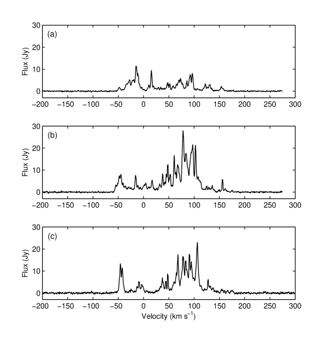
Figure 2: (a): H₂O maser spectrum of I18286 taken by the NRO 45 m telescope on 2006 April 20, the observation details can be found in Deguchi et al. (2007). (b) and (c): Same as (a), but taken on 2008 April 30 and 2010 April 2, respectively.

Figure 1 shows the VLBA spectra of I18286 H₂O maser emission in epochs A and F. The spectra were created by integrating the flux for all the velocity channels in the regions containing maser emission, using the imspec task in MIRIAD. Unlike W 43A, IRAS 19134$+$2131, IRAS 16342$-$3814 (Likkel et al. 1992) and IRAS 16552$-$3050 (Suárez et al. 2008) in which the H₂O maser spectra clearly show two clusters of emission peaks widely separated in velocity space (hereafter referred to as a “double-group profile” for convenience, note that they may not have exactly two peaks), the spectra of I18286 show emission peaks throughout the velocity range from $-50$ km s^-1 to 150 km s^-1. This profile characteristic is similar to that of OH 009.1$-$0.4 (Walsh et al. 2009), which is another known water fountain with many spectral groups of peaks. Figure 2 shows the spectra obtained from the NRO 45 m telescope observations in 2006, 2008 and 2010. It can be seen that the spectral profile changes rapidly with time but the overall velocity range of the H₂O maser emission remains the same over the four years (cf. Imai 2007). However, it is possible that there exist a few weak components with velocity greater than 150 km s^-1, which have not been detected in the VLBA observations. The integrated flux values from the single-dish and VLBA spectra are within the usual range of such radio observations ($\sim$30%). It allows us to be confident that the missing flux in our interferometric observations is not significant.

3.2 Spatial Distribution

The number of identified maser features in the VLBA observations was different from epoch to epoch, as listed in Table 2. The maximum number of features found in a single epoch was 143, which is more than the number collected from the first VLBA observation (Imai 2007). Few maser features survived over all the 6 epochs, but many existed in 2 to 3 consecutive epochs. In the current analysis, it is found that each of the features spans a velocity range of less than 10 spectral channels. The spatial position is obtained by performing a 2-dimensional Gaussian fit at the channel where the maximum flux of each feature is found (i.e. the brightest maser spot). For simplicity, this brightest maser spot of each feature is used in the proper motion calculation, and it is assumed representative of its corresponding feature. Therefore from now on whenever the term “maser feature” is used, it means “the brightest maser spot of the feature”. The maser spots have relatively simple brightness structures so most of them have similar sizes to that of the synthesized beam. Figure 3 shows the spatial distribution of the maser emission peaks. They extend across a region of about 200 mas, with the red-shifted and blue-shifted clusters of the peaks located at the southeast and northwest sides respectively. I18286 lies at a distance of approximately 4.0 kpc according to an annual parallax measurement (Imai et al., in preparation), so 200 mas is equivalent to a linear scale of $\sim$800 AU.

Some characteristics of the outflow pattern are shown in Figure 3, they are summarized as follows:

1. Most of the maser features (over 80% of the total number) are concentrated in two arcs stretching from the center of the structure to both the red-shifted and blue-shifted ends. The two arcs are located almost point-symmetrically with respect to the central part of the distribution. The line-of-sight velocities ($V_{\mbox{\scriptsize LSR}}$) change approximately continuously along the arcs. The features near to the center of the structure have $V_{\mbox{\scriptsize LSR}}$ close to the systemic velocity ($\sim 50$ km s^-1), while those further away have $V_{\mbox{\scriptsize LSR}}$ with larger offsets from the systemic velocity. This characteristic is unique to I18286 amongst all the known water fountains.

2. Some features, though having similar spatial distances from the center, are shown to have significantly different $V_{\mbox{\scriptsize LSR}}$ (difference $>50$ km s^-1). They are observed to be overlapping on both the northern and southern sides of the structure (Region I and II).

3. There are also a few maser features found in the areas loosely defined by Void I and II, which are separated from the two arcs.

Finally, there was one maser feature that survived in all epochs. Its $V_{\mbox{\scriptsize LSR}}$ in epochs A to F is 52.01 km s^-1, 51.58 km s^-1, 51.57 km s^-1, 51.57 km s^-1, 51.58 km s^-1 and 51.58 km s^-1, respectively. These values are in the middle of the whole velocity range of the emission spectrum. In addition, this feature is also near to the spatial center of the structure. Therefore its brightest maser spot has been chosen as a reference point (indicated as the origin in Figure 3); this enables easy comparison between different epochs when finding the proper motion of maser features.

3.3 Proper Motions

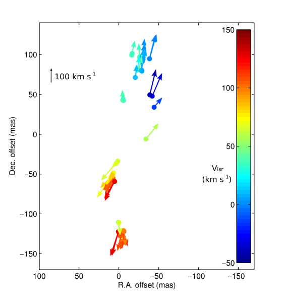
Figure 4: Proper motions of 54 H₂O maser features in I18286 which can be traced in any 3 consecutive epochs. The filled-circles represents the data in Table 3 with index 1.

Figure 4 shows the proper motions of 54 H₂O maser features identified in I18286. Most of them did not survive more than 3 epochs of the observations, with the exception of the chosen reference feature. The proper motions are therefore determined by tracing the features that existed in any 3 consecutive epochs, the velocities (as illustrated by the length of the vectors) are calculated by measuring the shift in position divided by the time over the mentioned period. The coordinates of the 54 maser features (represented by the brightest maser spot in each of them) in 3 different epochs are listed in Table 3. The proper motions reveal the bipolar nature of this water fountain, which is similar to W 43A (Imai et al. 2002) and IRAS 19134$+$2131 (Imai et al. 2007). The vectors all originate from the central region of the structure but it is obvious that they do not converge to a single point and there are notable deviations on the vectors’ directions (see Section 5.2). Table 4 lists the velocity information of these maser features; they are divided into two groups, which correspond to the proposed jet 1 and jet 2, respectively. More details are given in later sections.

4 Kinematic Modeling

It is difficult to propose a unique model using only the data available at the current time. However, any plausible model should be able to reproduce the three main characteristics of I18286 listed in Section 3.2. In the following, we examine models using these characteristics.

4.1 The Bipolar Precessing Jet Model

We propose a bipolar precessing jet model based on the fact that it can reproduce all three aforementioned characteristics. The bipolar jet is assumed to be point-symmetrical in the central part of the maser feature distribution. Qualitatively, precession will generate a helical jet pattern (e.g. the model of W 43A in Imai et al. 2002); the arc-shaped distribution of maser features can be explained by this phenomenon. In addition, as the jet precesses, the gas molecules are ejected in a 3D direction that varies at different instants. Therefore different regions of the arcs do not have the same $V_{\mbox{\scriptsize LSR}}$, which is just the projected velocity along the line-of-sight. The first characteristic is therefore well explained.

We propose that that the second and third characteristics could be reproduced by two modifications to the simple precessing jet model: (1) instead of a stationary driving source, we assume one that is moving; (2) we assume the ejection is episodic. These are reasonable assumptions as a source with significant proper motion is common, and episodic ejections in evolved stellar objects such as planetary nebulae have been observed before (e.g. López et al. 1995). Alternatively, we could assume the existence of two driving stars, rather than a single source with secular motion. Both models are explored in the discussion that follows.

The maser features in region I of Figure 3 can be divided into two groups based on $V_{\mbox{\scriptsize LSR}}$: those represented in “grey”, with $V_{\mbox{\scriptsize LSR}}$ roughly around 20 km s^-1 to 30 km s^-1; and those represented in “blue”, with $V_{\mbox{\scriptsize LSR}}$ $<0$. In region II, the same division is possible, in which there are distinct “yellow” and “red” maser features. The colorbar clearly shows that the two groups in both regions have very different $V_{\mbox{\scriptsize LSR}}$. We suggest the two groups are formed by different ejections of an episodic outflow, consistent with the above assumptions. For simplicity, we fit the jet pattern in the two ejection episodes independently by using two apparent jets.

The basic set of parametric equations for one bipolar jet is:

$$X_{\mathrm{R.A.}} = -V_{\mathrm{jet}}t\cos(\frac{2\pi t}{T})\sin\alpha+X_{0}~{};$$ (1)

$$Y_{\mathrm{Dec.}} = V_{\mathrm{jet}}t\cos\alpha+Y_{0}~{};$$ (2)

$$Z_{\mathrm{LOS}} = -V_{\mathrm{jet}}|t|\sin(\frac{2\pi t}{T})\sin\alpha+Z_{0}~{},$$ (3)

where $X_{\mathrm{R.A.}}$, $Y_{\mathrm{Dec.}}$ and $Z_{\mathrm{LOS}}$ (LOS stands for line-of-sight from the local standard of rest) are spatial coordinates of any point on the jet in 3D space, and $t$ is the time of travel to the supposed point. $t$ also acts as a running parameter linking eq. (1) to (3): when $t$ is positive, the equations represent the northern part of the bipolar jet; when $t$ is negative, the southern part is being considered. This set of equations is derived from the equations of a helix. A helix is chosen because mathematically this represents the spatial and kinematical pattern formed by a precession jet. The projected (2D) curves from the two model jets are used to fit the spatial and $V_{\mbox{\scriptsize LSR}}$ distribution of the H₂O maser features in each epoch independently. The free parameters for any model of the jets are the systemic LSR velocity of the jet ($V_{\mathrm{sys}}$, not shown in the equations, see below), precession period ($T$), precession angle ($\alpha$), position angle (P.A.) of the jet axis, the inclination angle (I.A.) of the axis with respect to the sky plane, and the position of the driving source, $X_{0}$ and $Y_{0}$. Since we are fitting the 2D projection only, $Z_{0}$ is set to 0. The jet velocity, $V_{\mathrm{jet}}$, is determined in the following way: the maser features listed in Table 4 are divided into two groups for each bipolar jet, one group is for the features that are travelling to the north, the other group is for those travelling to the south. The mean 3D velocity of each group is calculated, and $V_{\mathrm{jet}}$ is derived from the difference of the group velocities divided by 2. $V_{\mathrm{jet}}$ is assumed to be constant over the observation period. For jet 1, $V_{\mathrm{jet}}$ is equal to $138\pm 41$ km s^-1, and for jet 2 it is equal to $99\pm 21$ km s^-1. The resultant helix pattern can be spatially transformed and rotated (by Euler’s rotation) in order to find the position of the driving source and the jet’s axis direction such that the 2D projection of the model is best fitted with the observed maser distribution. The P.A. and I.A. can then be deduced from the Euler angles. Let $X^{\prime}_{\mathrm{R.A.}}$, $Y^{\prime}_{\mathrm{Dec.}}$ and $Z^{\prime}_{\mathrm{LOS}}$ be the new coordinates of each point on the jet model after any spatial transformation. Then the $V_{\mbox{\scriptsize LSR}}$ of each point is given by

$$V_{\mathrm{LSR}}=\frac{Z^{\prime}_{\mathrm{LOS}}}{t}+V_{\mathrm{sys}}~{}.$$ (4)

For the fitting, the dimensionless coefficient of determination, $R^{2}$, is used to measure the goodness of fit, where $R^{2}\leq 1$ (Steel & Torrie 1960).

In a normal curve fitting process, the data points only carry spatial information. However in our case, in addition to the R.A. and Dec., each point is also associated with a $V_{\mbox{\scriptsize LSR}}$ value that should not be neglected. Therefore the final $R^{2}$ is defined as

$$R^{2}=R^{2}_{\mathrm{spatial}}+R^{2}_{\mathrm{velocity}}~{},$$ (5)

where $R^{2}_{\mathrm{spatial}}$ measures the difference of the spatial component between the observation and the model; $R^{2}_{\mathrm{velocity}}$ measures the difference of the observed $V_{\mbox{\scriptsize LSR}}$ and that predicted in eq. (4). The weightings for the two $R^{2}$ components are set to 1, as we suggest that both spatial and $V_{\mbox{\scriptsize LSR}}$ information are equally important.

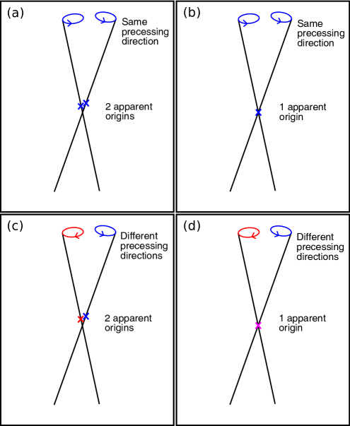
Figure 5: Four different possible scenarios for the precessing jet model. The main differences between each of them are the choice of precessing directions and the number of apparent jet origins.

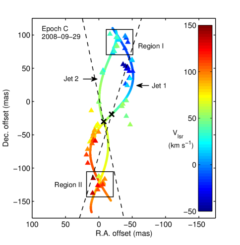
Figure 6: Illustration of the double precessing jet model with two resolvable driving sources, superposed on Figure 3. Since for every epoch the fitting procedure is the same, here only the fitted curve and maser data of epoch C are shown as an example. The two jets have the same anti-clockwise precessing direction. The black dotted lines show the projection of the jet axes on the sky plane. Jet 1 is the dominant jet with more H₂O maser features lying on it, while jet 2 is more subtle. The two driving sources (represented by two black crosses) are separated by $\sim$16 mas.

Figure 5 shows the schematic view of the four different possible scenarios for the model. Since we assume two jet patterns, we have to objectively consider all the cases in which they have different/similar apparent origins, and whether they have different/similar precessing directions. The best fit parameters are obtained by maximizing $R^{2}$. The fitting results of the four scenarios are shown in Table 5, and the graphical illustrations for different variations of the model are shown in Figure 6 to 8. Note that the small fitting errors listed in Table 5 only include the statistical variance from the fitting routine, and they give a 68% confidence level (1 sigma). Jet 1 is easily identified because many maser features can be found along nearly the whole jet, from the driving source up to the northern and southern tips, as shown in the figures. Statistically the fitting result for jet 1 is the most reliable among those presented in this paper, with $R^{2}=0.86$. The systemic velocity of the driving source is $\sim$47 km s^-1, and the precession period is $\sim$56 years. Jet 1 has a counter-clockwise precessing direction (note that in this paper, “clockwise” or “counter-clockwise” refers to the precessing direction observed from the northern side of the jet axis). On the contrary, in jet 2, few maser features appear in the region near to its driving source as most of them are located at the tips. In this case, it is numerically possible to fit several variations of the model to jet 2.

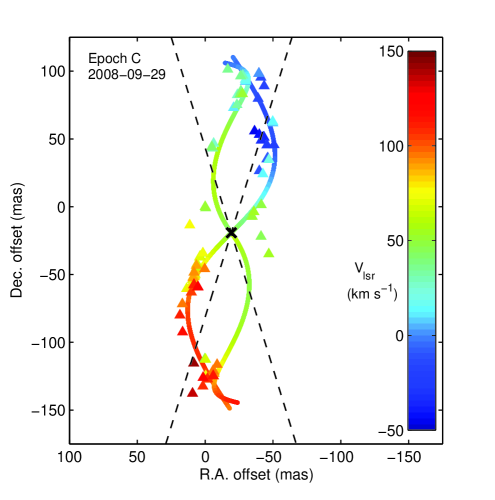
Figure 7: Same as Figure 6 but for the double precessing jet model with one driving source (i.e. the driving sources, even if there are more than one, are assumed to be unresolvable). The two jets have the same anti-clockwise precessing direction.

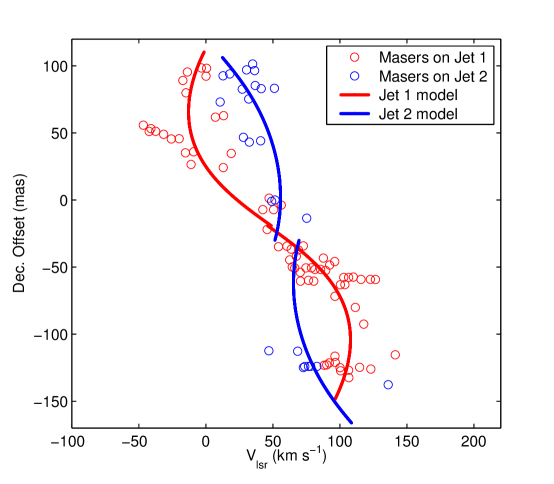
Figure 9: Declination offset of the maser features in epoch C against the corresponding line-of-sight velocities, together with the predicted values from the model fitting as shown in Figure 6. The data points and the model curve for jet 1 are represented by open-circles and line in red, while those for jet 2 are in blue. The declination of the reference maser feature is zero.

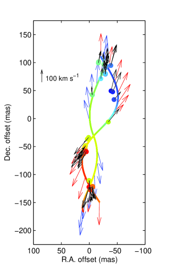
Figure 12: A comparison between the double-jet model in Figure 6 and the observed proper motions of H₂O maser features. Black arrows: Observed proper motions of I18286, which are the same as those illustrated in Figure 4. Red and blue arrows: Model predicted proper motions for maser features lying on jet 1 and jet 2.

From the model, jet 1 can reproduce the gradual change of the line-of-sight velocity of the maser features distributed along the helix curve, which is a typical pattern due to precession. For jet 2, there is not enough data, so even though we obtain reasonable values of $R^{2}$, the numerical results obtained by fitting might not be very accurate. Nonetheless, the existence of jet 2 should not be rejected solely because of the relatively small number of maser features. In fact, the inclusion of jet 2 in our model is necessary to explain a clear characteristic of the observations: in region I and II of Figure 6, the mixing of maser features with different line-of-sight velocities is well explained by the (apparently) overlapping effect of the two jets. The same thing happens for the two other scenarios as illustrated in Figure 7 and 8. In addition, the deviation of vector direction, as mentioned previously, can be interpreted by having two jets with different driving sources spatially close to each other as demonstrated by our model (be it resolvable or not). More support for our hypothesis is given in the three position-velocity diagrams (figure 9 to 11, jet $2a$ is chosen as an example as it gives the best $R^{2}$). It is observed that a single jet is not enough to describe the wide velocity distribution of the H₂O maser features at different positions. Figure 12 shows another qualitative comparison between the model predicted proper motions and the observed proper motions of the H₂O maser features. The model can correctly describe not only the spatial and $V_{\mathrm{LSR}}$ distribution (indicated by the colors), but the proper motions of the features as well (indicated by the arrows).

The best fit result for jet 2 is obtained when it is assumed that both jets are precessing in a counter-clockwise direction but originate from two resolvable driving sources (jet $2a$ in Table 5); in this case $R^{2}=0.73$. The systemic velocity and precession period for jet $2a$ are $\sim$61 km s^-1 and $\sim$73 years respectively, which are clearly different from those of jet 1. The second plausible case is that jet 2 precesses in the counter-clockwise direction and originates from the same point as jet 1 (jet $2b$ in Table 5). It does not necessarily mean that the two jets have physically the same driving source, but it represents the scenario in which the two sources are spatially unresolvable. Under this setting $R^{2}=0.54$, this is the lowest among all three trials. The systemic velocity is $\sim$54 km s^-1 and the precession period takes the value of $\sim$53 years, which is very close to that of jet 1. The third possible case is significantly different from the above two, jet 2 is now assumed to be precessing in an opposite direction to jet 1, i.e. in the clockwise direction, and they have two resolvable driving sources (jet $2c$ in Table 5). Even though the precessing direction is different, this model is able to produce a 2D projection well fitted with the observation. Here $R^{2}=0.70$, which is similar to the first case; the systemic velocity and precession period for jet $2c$ are $\sim$56 km s^-1 and $\sim$95 years respectively. This case has the longest precession period. Logically, there should be a fourth case, which corresponds to scenario (d) in Figure 5. In this case jet 2 has opposite precessing direction to jet 1 but they share the same origin point (i.e. unresolvable driving sources). However, it is found that the fitting result is untenable and so is not discussed further.

There are still some discrepancies between the model and the observations even if we fit two jets on the position-velocity diagrams, and the model cannot handle the few maser features that are scattered in the area near to the driving sources. They could hint at an as yet undiscovered equatorial outflow. Such an outflow associated with water fountains has been predicted by Imai (2007) to explain the existence of low velocity maser components in W 43A and IRAS 18460$-$0151, together with the narrow profile of the CO $J=3-2$ emission line in I18286 (Imai et al. 2009). Unfortunately, with only a few features identified in this area, quantitative analysis for this possible new component is out of the question for now, but at least we are confident that the masers are not lying on the proposed jets. If there are other kinematical components in addition to the jets, then the current model is not able to give very accurate answers. Nonetheless, the double-jet model offers one possible explanation for the observational results with a statistical basis. A discussion about the three different choices for jet 2 is given in Section 5.1.

4.2 Other Possibilities

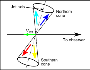
Figure 13: Illustration of the bi-cone model. The arrows show the outflow directions, and the colors indicate different line-of-sight velocities of the corresponding parts of the cone, with reference to the colorbar in Figure 3.

A bi-cone model, consisting of two jet cones connected by the tips, can also be tested. The bi-cone shape is typical in planetary nebula (Kwok 2008). If we assume water fountains play an important role in the shaping process as described in the introduction, the jet might somehow have a morphology similar to that of a planetary nebula. This model is simple in construction, and no unusual assumption is required. A schematic view of this model is given in Figure 13. If the jet axis is tilted as shown, then in the northern cone, the side closer to the observer has a larger red-shift than the opposite side. A similar argument can be applied to the blue-shifted southern cone. Therefore, the wide-angled jet cones are able to explain why there are maser features with significantly different $V_{\mbox{\scriptsize LSR}}$ appearing in the same region (e.g. region I and II) along the line-of-sight direction (i.e. the second characteristic of the outflow from I18286 listed in Section 3.2). However, this model cannot explain the continuously changing $V_{\mbox{\scriptsize LSR}}$ along the jet, the collimated arc-shaped distribution of the maser features, and the formation of the void regions (i.e. the first and third characteristics) and is therefore not considered further.

An outflow consisting of multiple outbursts could be another possible explanation to the maser distribution. However, to produce such large variations in the $V_{\mbox{\scriptsize LSR}}$ as shown in Figure 3, either the velocity of an individual outburst is very different from one to the other, or the jet axis is continually changing. It is difficult to explain such a physical condition, and we therefore consider such a model unfeasible.

5 Discussion

We have shown in the model that the maser distribution can be explained by two precessing jet patterns, but several questions remain unresolved. What is the origin of such jet patterns? What causes the spiky spectral profile of I18286? Such profiles are not commonly observed in water fountain sources but are often found in YSOs. How can we deduce the evolutionary status of this object? We have mentioned another water fountain with a precessing jet, W 43A, what are the similarities and differences between I18286 and W 43A? These questions are discussed in this section.

5.1 How to Produce Two Jet Patterns?

In Section 4.1, we demonstrated that the distribution and kinematic properties of the maser features can be explained by two precessing jet patterns. The scenario for jet 1 is quite clear, and for jet 2 three possible cases are investigated. Each of them gives a different set of best fit parameters (see Table 5) and naturally lead to different physical interpretations. The pros and cons of each case are discussed before we come to a conclusion.

Jet $2a$ in Table 5, for which $R^{2}=0.73$, gives the best fit model for jet 2. It is assumed in this model that jet 2 precesses in a counter-clockwise direction, similar to jet 1, but they have two resolvable driving sources separated by $\sim$16 mas (equivalent to 64 AU at 4 kpc). A possible scenario is that the “two” jets are actually formed by one single source but at different instants, and the source itself has a secular motion across the sky, moving from the position of jet $2a$’s driving source to that of jet 1 . This argument can explain why jet 2 has few maser features along the jet path other than at its tips. If the outflow is episodic, such that it will stop and resume after some time, the maser features at the tips of jet 2 mark the end of the previous ejection. The estimated “age” of this jet ($\sim$30 years) then reveals the time passed since this ejection. Jet 1 has a dynamical age of $\sim$19 years, which means at least 19 years ago the driving source was located at (or almost at) the current position, which is the fitted center of jet 1. In that case the driving source has taken less than 11 years to travel 64 AU (if only the projected 2D motion is considered), and its secular motion velocity is estimated to be $\sim$27 km s^-1, if constant. The deviation in the systemic velocity might favor the fact that the secular velocity is in fact changing. In that case the driving source is probably accelerated or has an orbital motion. Nonetheless, the idea of a positional shift for the driving source does not contradict previous observations of I18286.

The 3D velocity difference between jet 1 and jet 2 might also suggest that they represent two separate expulsion events. When the driving source is moving, the jet orientation with respect to Earth can vary. Therefore, the change in the projected jet axis (shown in Figure 6) between the events is not surprising. Figure 14 shows a schematic diagram of this moving-source model. The maser features that produce jet 2 are excited by the previous ejection, and as time passes they move to the tip of the jet leaving almost no traces along the path (the “void” regions of Figure 3). The OH maser, whose position is shown in Figure 3, is excited in the circumstellar envelope that moves along with the central star, and it provides an approximation of the latest position of the central star, which is consistent with our model. Jet 1 is “newly formed” and the ejection is probably still on going, therefore we can see the water maser features along the jet path, with the origin of jet 1 being the current position of the driving source. However, since the number of maser features associated with jet 2 is relatively small and they are concentrated at the tips, the fitting results have a larger uncertainty comparing to that of jet 1. This could be one of the reasons why jet 1 and jet $2a$ have different apparent precession angles and periods, while it is assumed that they are from the same source.

Jet $2b$ in Table 5 is the second possible case for modelling jet 2. It has almost the same construction as jet $2a$, but the number of apparent driving sources is different. In this scenario, jet 2 is also assumed to have the same precessing direction as jet 1 but this time both jets appear to originate from the same point, i.e. their driving sources are spatially unresolvable. Though the construction is similar, it is noted that the goodness of fit of jet $2b$ ($R^{2}=0.54$) is much worse than that of jet $2a$. It seems that the choice of having two resolvable/unresolvable driving sources is a crucial issue. Nonetheless, the same hypothesis as proposed for jet $2a$ can be applied here, and this time the problem of the discrepancy in precession period and precession angle does not occur as $T\sim 56$ years, $\alpha\sim 28$ degrees for jet 1, and $T\sim 53$ years, $\alpha\sim 22$ degrees for jet $2b$. The only difference between this scenario and that discussed above is the assumption that the proper motion of the driving source is too slow to be observed in this case, and thus it appears to be stationary.

Jet $2c$ in Table 5 is the third possible case, with $R^{2}=0.70$. The appearance of the fitted 2D curve looks similar to jet $2a$, but the two cases (i.e. jet $2a$ and $2c$) are actually quite different, as seen from the orientation of the jet axes (Figure 6 and 8). Here, jet 2 is assumed to be precessing in the opposite direction to jet 1, and the driving sources are spatially resolvable. In the previous model cases of jet $2a$ and $2b$, there is in fact only one jet with one driving source but it produces the pattern of two jets. This idea does not apply here because of the opposite precessing direction. Under this assumption we require two independent jets. This is kinematically possible and this time the missing maser features of jet 2 might be explained by the uneven distribution of ambient matter. The main problem is whether it is really physically possible to have two systems, of almost identical evolutionary status, launching jets in such close proximity. The two driving sources are separated by $\sim$17 mas (about 68 AU at 4 kpc), the radial separation is unknown.

The combination of jet 1 and jet $2a$ is the most plausible case from both a statistical and physical point of view. With the current data, we cannot expect this to be a unique model, but we believe it can satisfactorily explain the observational characteristics of I18286. In Section 4.1, we mentioned that it is possible to explain all the jet characteristics by using two independent driving sources. That would mean the two jet patterns are really formed by two different systems. It is clear that this construction gives us a lot of freedom in our modelling and the kinematical difference between jet 1 and jet 2 would be naturally explained. Nonetheless, this idea would imply that there are two “water fountain” objects at the same spot on the sky. We cannot totally reject this possibility, but given the fact that there are only 13 water fountains so far discovered across the sky, the probability of having two such objects at one site is very small. Hence we suggest that the two jet patterns are more likely coming from a single but moving source. Note that even though jet $2a$ and $2c$ have very different configurations, they both have their best fitted centers at similar locations. We believe this provides a constraint on the appropriate distance ($\sim$16 mas) between the two apparent driving sources, if they are resolvable. Finally, in our fitting, although the driving source(s) are assumed to be stationary for simplicity, this assumption does not contradict the above moving-source idea because the travelling speed of the driving source is slow compared with the jet velocity. A detailed kinematical model, which includes a travelling source, will be part of our future work.

5.2 The Feasibility of Having Two Resolvable Apparent Sources

From the above discussion, the models for jet $2a$ and $2b$ (i.e. one single jet forming the pattern of two jets) are seen to be most plausible. In the former case, the two jets are apparently driven from two resolvable sources in order to obtain reasonable $R^{2}$ values in the fitting. The remaining issue is whether this prediction of having two visually resolvable radiant points is feasible or not. A quantitative analysis is helpful for this matter.

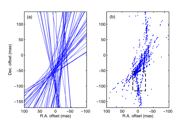
Figure 15: (a): The extensions of the proper motion vectors. Each straight line goes along the direction of a vector showing in Figure 4. (b): The interception points between any pair of straight lines as illustrated in (a). The driving sources are most likely lying within the dense region. The dotted black box denotes the “inverted triangle” feature, which is also found in Figure 16(b).

The straight lines in Figure 15 represent the extension of each proper motion vector as shown in Figure 4. For ballistic motion, if all the vectors originate from a single point, the straight lines should converge to one point. This happens when a single source model is being considered, or a model with two unresolvable sources (jet $2b$). The other case is of course, a model with two resolvable sources in which the straight lines should intercept at two distinct points. In reality, owing to the uncertainty of the maser positions, the observed proper motion for each maser feature has a measurement error and the extensions do not converge to one or two points only, instead the interception points for every pair of lines are distributed in an extended region around the real radiant point(s). The pattern in Figure 15(a) is therefore expected. However, this figure alone is inconclusive as the pattern can be generated by a single radiant point or two radiant points that are visually close to each other (e.g. jet $2a$).

We will build two simulation models, one with a pair of unresolvable driving sources (single apparent radiant point) and another one with a pair of resolvable driving sources, to compare them with the observations. Figure 15(b) shows the interception points for every two lines in Figure 15(a). The distribution of the points hints at the possible locations in which the dynamical centers could be found (i.e. the dense region at the center). The elongated pattern for the dense region is due to the bipolarity of the system (most of the maser features are concentrated along the north-south direction). As mentioned in the previous paragraph, one of the main reasons for the dispersion of the points is the error in the measured proper motion, this has to be taken into account for the models. The driving source for jet 1 is chosen as the single-radiant-point model due to its high degree of reliability as mentioned in the previous discussion. For the other model with two resolvable origins, we use the driving sources of jet 1 and jet $2a$ as the radiant points. In order to do a fair comparison, the same 54 maser features as listed in Table 3 are used for generating the “artificial” proper motions. The steps for one simulation of a model are as follows:

1. The maser features with index 1 in Table 3 are used, for simplicity, we group these coordinates as set A.

2. Assuming the features move along straight lines from the chosen radiant point(s), we can calculate the new positions of the features half a year later. This new set of coordinates are referred to as set B. Therefore, each member in set B represents the predicted location of each corresponding member in set A half year later, under ideal conditions.

3. Table 2 shows that the positional uncertainty of the maser features is $\sim$0.1 mas in all the epochs. Therefore, in order to reproduce the positional uncertainties in the real observables, random “errors” following a 2D Gaussian distribution with $\sigma=0.1$ mas are added to all the coordinates in set B.

4. Now we have two epochs of data, set A and B. We can calculate the proper motions and make a map similar to Figure 15(b). The data points here are grouped in set C.

The above steps are repeated 1000 times for both models.

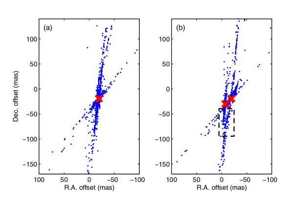
Figure 16: (a): Similar to Figure 15(b), but the data are generated by a model with a single radiant point (to represent the case where the two driving sources are unresolvable) The cross indicates the location of the assumed single radiant point, which has the coordinates of the driving source for jet 1. (b): Similar to (a), but the model has two resolvable radiant points. The red crosses indicate the positions of the driving sources of jet 1 and jet $2a$. The dotted black box denotes the “inverted triangle” feature, which is also found in Figure 15(b).

Figure 16(a) shows one of the simulation results (set C) for the model with unresolvable driving sources, and Figure 16(b) shows the result for the model with resolvable driving sources. The model for the resolvable case is able to reproduce the “inverted triangle” feature found in the observation data (indicated by the dotted black boxes in Figure 15(b) and 16(b)), while the other fails to do so. To produce this feature, two different trends of proper motions are needed and therefore only the resolvable case could fulfil this criteria.

For further analysis, each time set C is obtained, it is compared with the observed data (Figure 15(b)) by the Kolmogorov-Smirnov test (or K-S test, see for example, Lupton 1993). The “bins” of the K-S test are assigned in such a way that each bin represents different distances between a data point to the radiant point(s), with a resolution of 1 mas bin^-1. The averaged p-value, which represents the null hypothesis of the two sets of data being “the same”, has a value of 5% for the unresolvable-driving-sources model, while for the resolvable case, the value is 51%. We believe that the unresolvable case can be rejected with a 95% confidence level.

The above results are therefore consistent with the idea of having two resolvable radiant points, and the jet 1 and jet $2a$ combination remains as a plausible explanation to the observed maser distribution, even though some of the parameters require confirmation. Finally, it should be noted that the crossing of the two jets in region I and II of Figure 6 is just a visual effect, the jets actually do not meet as seen from our 3D version of the model. In fact, if the jets really collide with each other, the maser kinematics in the colliding regions would be more complicated than that observed.

5.3 Evolutionary Status and a Comparison with W 43A

I18286 appears as a very red point source in both MSX and GLIMPSE images (Deguchi et al. 2007). Its position on the MSX color-color diagram suggests that it is an evolved star (see, e.g. Figure 3 in Day et al. 2010). However, I18286 exhibits a spiky spectral profile as presented in Figure 1; such a line profile, showing a number of peaks, is not typical in AGB and post-AGB stars, but is often found in star forming regions. Therefore, it is necessary to consider some basic characteristics of I18286 to understand its evolved star status before undertaking any further interpretation with this assumption.

Even though many YSOs also have a spiky spectral profile, their velocity range is quite different. Water fountains such as I18286 and other examples mentioned in this paper exhibit H₂O spectra with a large velocity range ($\geq$100 km s^-1), while for many YSOs the range is usually less than 50 km s^-1 (see, for example, Ellingsen et al. 2010, Urquhart et al. 2009). Nonetheless, there are cases such as W 49 (McGrath et al. 2004) and W 51 (Genzel et al. 1979) in which the spectra show emission peaks spread across 100 km s^-1 or more, so only considering the velocity range is not sufficient to determine whether I18286 is an evolved star or a YSO. However, for YSO spectra, the high velocity H₂O maser features are usually significantly weaker in flux than those at low velocity. This is not the case for I18286  where its spectra show bright peaks in the high velocity range (Figure 1).

In addition, the NRAO VLA Sky Survey at 1.4 GHz ($\lambda=21$ cm) shows no continuum detection in the direction of I18286 (Condon et al. 1998), which means it has no significant H_II source there and hence the object is unlikely to be lying in a high-mass star forming region. The report on the detection of 1612 MHz OH maser by Sevenster et al. (1997) also suggests that I18286 is not a low-mass YSO, as there are currently no such OH masers found in this type of object (Sahai et al. 2007). Therefore, I18286 is likely to be an evolved star.

I18286 is the second example of a water fountain other than W 43A in which a highly collimated precessing outflow is observed. Imai et al. (2002) state that the molecular jet of W 43A has a precession period of 55 years and an outflow velocity of about 150 km s^-1. These values are of the same order of magnitude as the jet(s) in I18286 (see Table 5). It is unclear whether the similar kinematic parameters are just a coincidence or that there is a physical reason behind it. However, it is worth looking at the similarities and differences between the two objects. The properties of the H₂O and OH masers are discussed below.

The H₂O maser features of W 43A are found in two well separated clusters on spatial maps, and they show a double-group spectral profile, which is common in water fountains as mentioned previously. Generally, H₂O maser emission is thought to be found in a shocked region which is formed by the collision between an outflowing jet and the ambient gas of the star (Elitzur 1992). For water fountains such as W 43A, this happens at the tips of the bipolar jets with high velocity, hence the double-group profile is produced, and the maser features appear to be collected in two isolated clusters on spatial maps. In the case of I18286, however, other than the spiky spectral profile, the maser features seem to trace the jet starting from the region close to the central star all the way up to the blue-shifted and red-shifted tips, as indicated in the spatial distribution of maser emission (Figure 3). If the inner-wall of the ambient gas envelope is relatively close to the central star, H₂O maser excitation would occur in the vicinity of the star and move along with the jet penetrating into the gas envelope. The whole jet can then be traced out by maser emission. Furthermore, if the maser features have different line-of-sight velocities in various positions on the jet (as in the case of a precessing jet), a spiky profile with emission peaks of different velocities will be observed (Figure 1).

Imai et al. (2008) reports on VLBI observations of 1612 MHz OH maser for both W 43A and I18286. The spatio-kinematical structure of the OH maser emission associated with W 43A can be described as a spherically expanding shell with an expansion velocity of $\sim$9 km s^-1 and radius of 500 AU, assuming a distance of 2.6 kpc. For I18286, only a single emission peak was detected with line-of-sight velocity equal to 39.5 km s^-1. If we assume that the OH maser detection is also part of a spherical expanding shell, then the expansion velocity is estimated to be $\sim$7.5 km s^-1 if the line-of-sight velocity for the central star of I18286 is taken as $\sim$47 km s^-1 ($V_{\mathrm{sys}}$ of jet 1). The ambient shells of the two objects then have similar expansion velocities.

6 Conclusions

Our VLBA observations reveal a double-helix pattern traced by 22.2 GHz H₂O maser emission. Modelling results show that the pattern can be fit by two bipolar precessing ballistic jets. Jet 1 has a period of $\sim$56 years which is similar to that of W 43A (Imai et al. 2002), while jet 2 has a longer period of $\sim$73 years (if the case of jet $2a$ is adopted). The two apparent driving sources are separated by $\sim$16 mas on the sky plane, which is about 64 AU at 4 kpc. From the proper motions of the maser features, the 3D jet velocities are found to be $\sim$138 km s^-1 and $\sim$99 km s^-1 for jet 1 and jet 2 respectively, if they are assumed to be constant throughout the observation period. It is suggested from the above analysis that there is in fact one driving source only, but its secular motion and the episodic outflow possibly produce the two jet patterns. I18286 is likely to be an evolved star because of the wide velocity span of the H₂O maser emission, the detection of a 1612 MHz OH maser and its infrared characteristics. Further investigation is needed to search for the existence of an equatorial outflow as hinted by the maser detection near to the driving sources but not lying on the jets. It is also worth obtaining additional interferometry data covering the high velocity components that have not been included in the current VLBA results. An enhanced model, which includes the possible proper motion of the driving source, could be used in our future analysis. The discovery of I18286 shows that a precessing collimated jet is not just confined to W 43A. These two objects have kinematical similarities, and it may mean that there are specific conditions for precessing jets to occur, but they are yet to be discovered.

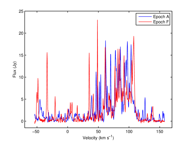
Figure 1: H₂O maser spectra of I18286 in epoch A (2008 April 21) and F (2009 May 19) of the VLBA observations. The spectra are created by the MIRIAD task IMSPEC, and the integration regions are selected in a way such that all the maser features are included. The spectrum for epoch A is displayed in blue while that for epoch F is in red. The spiky profile is one of the characteristics of I18286. Emission peaks are found in the range of $-50$ km s^-1 to $150$ km s^-1 for all the epochs, but a significant change in the profile is noticed over the observation period.

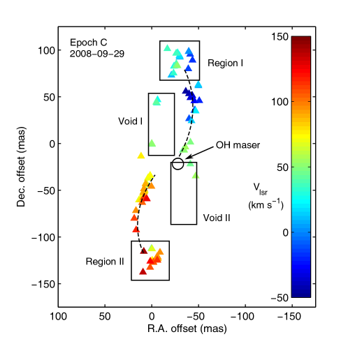
Figure 3: Spatial distribution of I18286 H₂O maser features in Epoch C. Since the appearance looks very similar for all epochs, only this one is shown here. In Epoch C, most of the features with measured proper motions were detected. (shown in Figure 4). Each maser feature is represented by a filled-triangle and the color denotes its line-of-sight velocity according to the scale of the color bar. Most of the maser features are lying on the two dotted arcs, but in Void I and Void II only a few of them are found. Region I and Region II show clusters of maser features with wide ranges of line-of-sight velocities ($-40$ km s^-1$\,<\,$$V_{\mbox{\scriptsize LSR}}$$\,<40$ km s^-1 and $70$ km s^-1$\,<\,$$V_{\mbox{\scriptsize LSR}}$$\,<150$ km s^-1, at the northern and southern end of the structure, respectively). The map origin is set at the chosen reference feature. The black circle indicates the position of the OH maser emission (Imai et al. 2008).

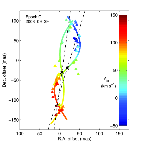
Figure 8: Same as Figure 6 but the two jets have opposite precessing directions. The two driving sources (represented by two black crosses) are separated by $\sim$17 mas.

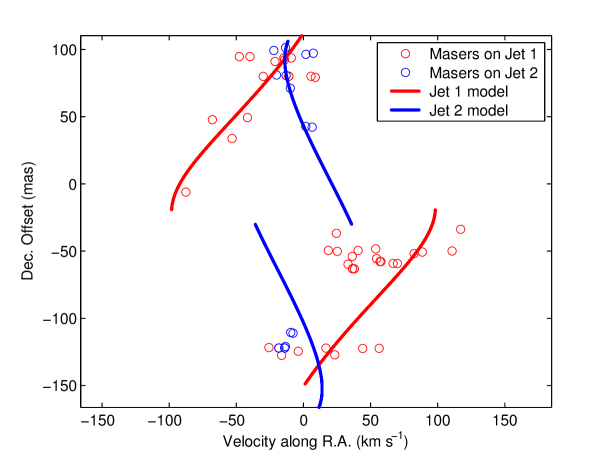
Figure 10: Same as Figure 10 but for the declination of the maser features in Figure 4 against the corresponding proper motion velocities along the R.A. direction, together with the predicted values from the model fitting as shown in Figure 6.

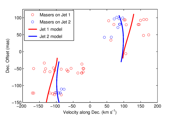
Figure 11: Same as Figure 10 but for the declination of the maser features in Figure 4 against the corresponding proper motion velocities along the Dec. direction, together with the predicted values from the model fitting as shown in Figure 6.

Figure 14: Illustration of the moving-source model which produces two jet patterns from one driving source only.

Table 1: Parameters of the VLBA observations and data reduction for each individual epoch.

Observation	Epoch			Beam
code	(yyyy-mm-dd)	$V_{\mbox{\scriptsize ref}}$	Noise	(mas)	$N_{\mbox{\scriptsize f}}$
BI37A	2008-04-21	59.8	1.1	1.81$\times$1.05, $-1\fdg$5	143
BI37B	2008-05-29	59.8	4.9	3.09$\times$1.47, 15$\fdg$0	120
BI37C	2008-09-29	42.5	2.7	1.99$\times$1.12, 25$\fdg$9	94
BI37D	2008-11-28	43.3	1.0	2.31$\times$1.33, 22$\fdg$5	134
BI37E	2009-02-13	51.6	16.9	3.28$\times$1.48, 16$\fdg$2	41
BI37F	2009-05-19	61.3	16.9	3.28$\times$1.48, 16$\fdg$2	97

Table 2: Parameters of the brightest H₂O maser spot from each detected maser feature in epoch A to F (see Section 3 for details).

$V_{\mbox{\tiny LSR}}$	R.A. offset		Decl. offset		$I$
(km s-1)	(mas)		(mas)
2008 April 21 (epoch A)
$-50.75$	$-39.45$ $\pm$	$0.04$	$49.40$ $\pm$	$0.09$	$0.42$
$-51.17$	$-43.79$ $\pm$	$0.07$	$68.31$ $\pm$	$0.08$	$1.03$
$-49.69$	$-39.96$ $\pm$	$0.04$	$57.82$ $\pm$	$0.04$	$0.39$
$-44.42$	$-38.15$ $\pm$	$0.04$	$49.98$ $\pm$	$0.05$	$2.10$
$-45.47$	$-35.04$ $\pm$	$0.01$	$53.01$ $\pm$	$0.04$	$1.98$
$-42.94$	$-38.95$ $\pm$	$0.01$	$49.44$ $\pm$	$0.06$	$1.78$
$-39.57$	$-40.84$ $\pm$	$0.02$	$51.32$ $\pm$	$0.07$	$1.18$
$-40.20$	$-45.21$ $\pm$	$0.06$	$56.78$ $\pm$	$0.07$	$0.55$
$-37.03$	$-41.92$ $\pm$	$0.03$	$47.79$ $\pm$	$0.02$	$0.65$
$-33.66$	$-40.89$ $\pm$	$0.08$	$36.99$ $\pm$	$0.08$	$0.41$
$-33.66$	$-41.30$ $\pm$	$0.08$	$47.24$ $\pm$	$0.01$	$0.51$
$-31.13$	$-40.88$ $\pm$	$0.09$	$46.52$ $\pm$	$0.04$	$1.39$
$-30.49$	$-38.40$ $\pm$	$0.05$	$44.97$ $\pm$	$0.07$	$0.63$
$-28.81$	$-44.17$ $\pm$	$0.03$	$67.67$ $\pm$	$0.07$	$0.81$
$-25.43$	$-38.49$ $\pm$	$0.03$	$22.98$ $\pm$	$0.04$	$0.85$
$-23.53$	$-48.51$ $\pm$	$0.05$	$54.10$ $\pm$	$0.07$	$0.43$
$-18.89$	$-34.21$ $\pm$	$0.07$	$89.68$ $\pm$	$0.08$	$0.61$
$-16.78$	$-40.92$ $\pm$	$0.04$	$23.30$ $\pm$	$0.03$	$0.32$
$-15.51$	$-34.29$ $\pm$	$0.05$	$89.65$ $\pm$	$0.02$	$1.18$
$-14.04$	$-39.93$ $\pm$	$0.06$	$92.28$ $\pm$	$0.03$	$1.11$
$-13.61$	$-44.36$ $\pm$	$0.08$	$33.86$ $\pm$	$0.04$	$0.89$
$-5.17$	$-42.38$ $\pm$	$0.02$	$85.96$ $\pm$	$0.03$	$0.34$
$-4.12$	$-40.05$ $\pm$	$0.07$	$93.65$ $\pm$	$0.08$	$1.48$
$-0.53$	$-38.58$ $\pm$	$0.06$	$94.80$ $\pm$	$0.01$	$1.33$
$1.58$	$-48.60$ $\pm$	$0.04$	$58.06$ $\pm$	$0.06$	$0.47$
$3.69$	$-48.36$ $\pm$	$0.08$	$58.84$ $\pm$	$0.02$	$0.76$
$46.73$	$-34.02$ $\pm$	$0.04$	$-7.06$ $\pm$	$0.08$	$1.22$
$46.31$	$-40.33$ $\pm$	$0.02$	$1.16$ $\pm$	$0.02$	$4.82$
$49.05$	$-33.98$ $\pm$	$0.06$	$-7.20$ $\pm$	$0.05$	$5.55$
$53.91$	$-38.49$ $\pm$	$0.06$	$9.78$ $\pm$	$0.09$	$0.46$
$53.69$	$-42.11$ $\pm$	$0.04$	$15.32$ $\pm$	$0.04$	$1.84$
$56.65$	$-34.09$ $\pm$	$0.07$	$-6.06$ $\pm$	$0.01$	$1.18$
$57.28$	$-42.27$ $\pm$	$0.09$	$15.46$ $\pm$	$0.03$	$0.76$
$60.03$	$-41.77$ $\pm$	$0.09$	$13.82$ $\pm$	$0.04$	$0.67$
$53.91$	$-46.28$ $\pm$	$0.02$	$-34.62$ $\pm$	$0.04$	$5.31$
$-25.85$	$-31.00$ $\pm$	$0.03$	$60.09$ $\pm$	$0.03$	$0.66$
$-9.82$	$-31.38$ $\pm$	$0.01$	$90.74$ $\pm$	$0.08$	$0.75$
$-7.07$	$-30.93$ $\pm$	$0.06$	$90.87$ $\pm$	$0.06$	$0.31$
$1.58$	$-29.31$ $\pm$	$0.02$	$91.16$ $\pm$	$0.09$	$1.71$
$4.32$	$-27.59$ $\pm$	$0.04$	$75.67$ $\pm$	$0.05$	$1.06$
$5.38$	$-29.71$ $\pm$	$0.08$	$91.46$ $\pm$	$0.09$	$0.83$
$11.28$	$-20.75$ $\pm$	$0.05$	$71.26$ $\pm$	$0.01$	$1.25$
$12.97$	$-30.11$ $\pm$	$0.04$	$91.05$ $\pm$	$0.06$	$1.31$
$19.09$	$-16.40$ $\pm$	$0.03$	$49.53$ $\pm$	$0.07$	$0.86$
$19.09$	$-27.85$ $\pm$	$0.05$	$79.74$ $\pm$	$0.03$	$0.55$
$18.04$	$-27.99$ $\pm$	$0.09$	$89.65$ $\pm$	$0.08$	$0.94$
$20.15$	$-12.18$ $\pm$	$0.02$	$55.01$ $\pm$	$0.07$	$0.68$
$22.26$	$-22.34$ $\pm$	$0.05$	$78.48$ $\pm$	$0.08$	$0.41$
$27.95$	$-6.41$ $\pm$	$0.08$	$45.75$ $\pm$	$0.06$	$0.33$
$27.11$	$-23.47$ $\pm$	$0.01$	$80.75$ $\pm$	$0.07$	$1.25$
$27.95$	$-28.00$ $\pm$	$0.07$	$93.42$ $\pm$	$0.04$	$0.53$
$31.75$	$-5.66$ $\pm$	$0.09$	$42.28$ $\pm$	$0.03$	$0.73$
$31.12$	$-33.26$ $\pm$	$0.03$	$99.31$ $\pm$	$0.03$	$0.33$
$33.65$	$-24.60$ $\pm$	$0.02$	$81.68$ $\pm$	$0.06$	$1.15$
$33.23$	$-29.09$ $\pm$	$0.06$	$95.23$ $\pm$	$0.08$	$0.64$
$36.60$	$-27.31$ $\pm$	$0.08$	$95.07$ $\pm$	$0.03$	$0.95$
$35.55$	$-16.21$ $\pm$	$0.06$	$99.32$ $\pm$	$0.04$	$0.59$
$37.66$	$-5.62$ $\pm$	$0.08$	$42.09$ $\pm$	$0.08$	$0.74$
$38.29$	$-26.01$ $\pm$	$0.03$	$94.38$ $\pm$	$0.06$	$1.50$
$40.61$	$-4.91$ $\pm$	$0.07$	$42.77$ $\pm$	$0.09$	$0.59$
$39.35$	$-23.85$ $\pm$	$0.04$	$75.97$ $\pm$	$0.03$	$3.97$
$40.19$	$-27.11$ $\pm$	$0.04$	$94.97$ $\pm$	$0.08$	$0.45$
$41.03$	$-25.25$ $\pm$	$0.02$	$81.08$ $\pm$	$0.06$	$1.12$
$44.20$	$-24.93$ $\pm$	$0.08$	$75.51$ $\pm$	$0.03$	$1.55$
$43.15$	$-30.22$ $\pm$	$0.06$	$93.29$ $\pm$	$0.05$	$0.38$
$47.15$	$-27.17$ $\pm$	$0.07$	$81.69$ $\pm$	$0.04$	$0.73$
$48.63$	$-0.33$ $\pm$	$0.07$	$-0.99$ $\pm$	$0.06$	$0.81$
$52.01$	$0$ $\pm$	$0.02$	$0$ $\pm$	$0.07$	$4.35$
$51.80$	$-25.71$ $\pm$	$0.09$	$80.44$ $\pm$	$0.02$	$1.68$
$61.92$	$6.51$ $\pm$	$0.05$	$-1.19$ $\pm$	$0.08$	$0.34$
$62.98$	$-19.47$ $\pm$	$0.07$	$67.06$ $\pm$	$0.08$	$0.33$
$97.37$	$9.08$ $\pm$	$0.07$	$6.70$ $\pm$	$0.04$	$0.33$
$43.57$	$4.49$ $\pm$	$0.08$	$-101.47$ $\pm$	$0.04$	$0.55$
$44.83$	$9.73$ $\pm$	$0.02$	$-61.42$ $\pm$	$0.06$	$0.36$
$46.73$	$0.47$ $\pm$	$0.05$	$-110.51$ $\pm$	$0.07$	$0.64$
$59.81$	$-29.69$ $\pm$	$0.06$	$-12.61$ $\pm$	$0.07$	$0.93$
$61.71$	$-4.20$ $\pm$	$0.08$	$-72.09$ $\pm$	$0.07$	$0.41$
$61.71$	$2.65$ $\pm$	$0.08$	$-35.72$ $\pm$	$0.04$	$11.36$
$61.71$	$-1.11$ $\pm$	$0.08$	$-28.53$ $\pm$	$0.04$	$0.35$
$63.19$	$-30.52$ $\pm$	$0.06$	$-11.90$ $\pm$	$0.09$	$1.07$
$66.14$	$-0.19$ $\pm$	$0.06$	$-111.02$ $\pm$	$0.06$	$0.71$
$64.25$	$7.07$ $\pm$	$0.08$	$-49.45$ $\pm$	$0.08$	$0.71$
$64.67$	$1.20$ $\pm$	$0.01$	$-33.72$ $\pm$	$0.03$	$5.10$
$67.20$	$8.31$ $\pm$	$0.08$	$-51.69$ $\pm$	$0.06$	$0.82$
$67.20$	$3.55$ $\pm$	$0.04$	$-36.69$ $\pm$	$0.06$	$1.38$
$67.41$	$-31.59$ $\pm$	$0.01$	$-11.36$ $\pm$	$0.09$	$0.39$
$69.94$	$-0.96$ $\pm$	$0.07$	$-122.82$ $\pm$	$0.02$	$10.60$
$69.31$	$9.29$ $\pm$	$0.02$	$-55.70$ $\pm$	$0.05$	$0.77$
$70.79$	$13.40$ $\pm$	$0.02$	$-59.95$ $\pm$	$0.05$	$0.39$
$71.42$	$9.66$ $\pm$	$0.06$	$-46.47$ $\pm$	$0.02$	$0.40$
$71.21$	$5.20$ $\pm$	$0.03$	$-40.97$ $\pm$	$0.08$	$0.96$
$73.95$	$6.78$ $\pm$	$0.04$	$-48.28$ $\pm$	$0.08$	$2.24$
$75.43$	$11.25$ $\pm$	$0.04$	$-13.58$ $\pm$	$0.05$	$0.32$
$77.96$	$-4.21$ $\pm$	$0.04$	$-122.03$ $\pm$	$0.07$	$6.31$
$77.75$	$-0.25$ $\pm$	$0.04$	$-87.80$ $\pm$	$0.02$	$0.38$
$77.75$	$3.47$ $\pm$	$0.06$	$-84.80$ $\pm$	$0.06$	$0.38$
$79.01$	$0.51$ $\pm$	$0.02$	$-87.16$ $\pm$	$0.03$	$0.36$
$79.65$	$7.48$ $\pm$	$0.03$	$-50.16$ $\pm$	$0.05$	$7.08$
$81.97$	$1.12$ $\pm$	$0.02$	$-86.42$ $\pm$	$0.08$	$0.39$
$81.12$	$11.51$ $\pm$	$0.04$	$-60.61$ $\pm$	$0.03$	$1.19$
$82.18$	$7.75$ $\pm$	$0.07$	$-49.98$ $\pm$	$0.03$	$6.81$
$83.24$	$-6.70$ $\pm$	$0.03$	$-120.17$ $\pm$	$0.05$	$2.57$
$84.08$	$8.32$ $\pm$	$0.07$	$-53.31$ $\pm$	$0.04$	$7.81$
$85.35$	$-0.12$ $\pm$	$0.07$	$-125.54$ $\pm$	$0.07$	$1.07$
$86.19$	$13.16$ $\pm$	$0.08$	$-63.78$ $\pm$	$0.09$	$0.51$
$85.98$	$8.33$ $\pm$	$0.08$	$-53.40$ $\pm$	$0.02$	$9.76$
$85.98$	$16.17$ $\pm$	$0.03$	$-16.17$ $\pm$	$0.03$	$0.42$
$87.67$	$-7.85$ $\pm$	$0.03$	$-122.46$ $\pm$	$0.07$	$0.95$
$89.35$	$8.28$ $\pm$	$0.05$	$-53.49$ $\pm$	$0.04$	$3.66$
$91.04$	$-5.93$ $\pm$	$0.04$	$-120.95$ $\pm$	$0.09$	$1.70$
$92.73$	$8.85$ $\pm$	$0.08$	$-60.20$ $\pm$	$0.09$	$8.24$
$95.47$	$-5.82$ $\pm$	$0.07$	$-119.20$ $\pm$	$0.06$	$1.21$
$96.95$	$-1.49$ $\pm$	$0.05$	$-124.97$ $\pm$	$0.08$	$2.68$
$97.16$	$5.31$ $\pm$	$0.03$	$-96.65$ $\pm$	$0.04$	$0.34$
$97.16$	$-2.34$ $\pm$	$0.06$	$-84.99$ $\pm$	$0.06$	$0.34$
$97.58$	$9.31$ $\pm$	$0.03$	$-62.01$ $\pm$	$0.09$	$9.68$
$100.33$	$-1.63$ $\pm$	$0.05$	$-124.71$ $\pm$	$0.05$	$2.63$
$100.54$	$7.16$ $\pm$	$0.04$	$-55.44$ $\pm$	$0.08$	$3.12$
$103.49$	$-1.60$ $\pm$	$0.05$	$-131.93$ $\pm$	$0.07$	$0.33$
$103.49$	$-1.58$ $\pm$	$0.09$	$-124.63$ $\pm$	$0.05$	$4.07$
$102.65$	$2.36$ $\pm$	$0.07$	$-98.45$ $\pm$	$0.06$	$0.34$
$103.28$	$9.20$ $\pm$	$0.09$	$-62.19$ $\pm$	$0.08$	$8.35$
$108.13$	$-1.66$ $\pm$	$0.03$	$-124.45$ $\pm$	$0.03$	$3.22$
$107.08$	$7.14$ $\pm$	$0.05$	$-55.33$ $\pm$	$0.04$	$0.46$
$114.04$	$-6.29$ $\pm$	$0.01$	$-122.15$ $\pm$	$0.09$	$0.35$
$114.88$	$15.59$ $\pm$	$0.07$	$-108.03$ $\pm$	$0.04$	$1.85$
$120.16$	$-1.67$ $\pm$	$0.06$	$-123.34$ $\pm$	$0.06$	$0.46$
$119.53$	$15.49$ $\pm$	$0.08$	$-107.69$ $\pm$	$0.08$	$0.33$
$122.48$	$0.32$ $\pm$	$0.09$	$-122.29$ $\pm$	$0.09$	$0.55$
$122.27$	$16.21$ $\pm$	$0.08$	$-109.37$ $\pm$	$0.06$	$1.56$
$122.06$	$17.85$ $\pm$	$0.04$	$-86.36$ $\pm$	$0.02$	$0.34$
$126.07$	$0.58$ $\pm$	$0.01$	$-122.37$ $\pm$	$0.01$	$0.88$
$126.07$	$16.21$ $\pm$	$0.05$	$-109.42$ $\pm$	$0.06$	$3.00$
$130.50$	$15.03$ $\pm$	$0.03$	$-107.81$ $\pm$	$0.06$	$0.65$
$130.92$	$16.95$ $\pm$	$0.03$	$-85.52$ $\pm$	$0.09$	$0.37$
$133.88$	$-0.96$ $\pm$	$0.04$	$-120.61$ $\pm$	$0.07$	$0.37$
$137.88$	$9.30$ $\pm$	$0.02$	$-134.12$ $\pm$	$0.06$	$0.49$
$137.04$	$15.80$ $\pm$	$0.07$	$-119.27$ $\pm$	$0.05$	$0.50$
$136.83$	$15.16$ $\pm$	$0.07$	$-107.60$ $\pm$	$0.03$	$2.02$
$140.84$	$15.28$ $\pm$	$0.05$	$-107.57$ $\pm$	$0.09$	$0.70$
$149.49$	$15.22$ $\pm$	$0.04$	$-106.89$ $\pm$	$0.05$	$1.48$
$156.66$	$7.25$ $\pm$	$0.08$	$-128.14$ $\pm$	$0.01$	$1.42$
$155.19$	$15.23$ $\pm$	$0.05$	$-106.72$ $\pm$	$0.07$	$1.76$
2008 May 29 (epoch B)
$-48.85$	$-35.59$ $\pm$	$0.05$	$53.07$ $\pm$	$0.02$	$2.87$
$-44.21$	$-39.21$ $\pm$	$0.01$	$50.88$ $\pm$	$0.03$	$1.26$
$-39.57$	$-42.31$ $\pm$	$0.08$	$48.77$ $\pm$	$0.02$	$2.72$
$-37.46$	$-41.57$ $\pm$	$0.04$	$39.49$ $\pm$	$0.06$	$0.35$
$-38.09$	$-45.61$ $\pm$	$0.03$	$57.62$ $\pm$	$0.02$	$1.83$
$-35.56$	$-45.69$ $\pm$	$0.02$	$57.18$ $\pm$	$0.08$	$0.43$
$-34.51$	$-40.15$ $\pm$	$0.03$	$49.08$ $\pm$	$0.07$	$0.84$
$-31.76$	$-39.65$ $\pm$	$0.03$	$22.71$ $\pm$	$0.08$	$0.44$
$-32.82$	$-41.50$ $\pm$	$0.06$	$38.97$ $\pm$	$0.05$	$0.33$
$-29.02$	$-39.51$ $\pm$	$0.02$	$23.07$ $\pm$	$0.06$	$0.42$
$-28.81$	$-38.42$ $\pm$	$0.03$	$45.53$ $\pm$	$0.08$	$0.92$
$-28.60$	$-41.97$ $\pm$	$0.03$	$35.88$ $\pm$	$0.05$	$1.26$
$-25.01$	$-39.35$ $\pm$	$0.08$	$23.06$ $\pm$	$0.03$	$0.39$
$-23.96$	$-39.42$ $\pm$	$0.05$	$49.12$ $\pm$	$0.09$	$0.79$
$-20.58$	$-42.60$ $\pm$	$0.07$	$86.59$ $\pm$	$0.01$	$0.48$
$-19.53$	$-39.98$ $\pm$	$0.06$	$48.96$ $\pm$	$0.04$	$0.83$
$-16.99$	$-39.04$ $\pm$	$0.07$	$23.72$ $\pm$	$0.09$	$0.37$
$-17.84$	$-34.48$ $\pm$	$0.02$	$90.50$ $\pm$	$0.04$	$1.75$
$-15.94$	$-34.43$ $\pm$	$0.09$	$90.48$ $\pm$	$0.03$	$0.61$
$-14.67$	$-40.48$ $\pm$	$0.08$	$92.91$ $\pm$	$0.02$	$0.36$
$-12.98$	$-40.30$ $\pm$	$0.01$	$23.16$ $\pm$	$0.08$	$1.54$
$-12.56$	$-44.75$ $\pm$	$0.05$	$34.35$ $\pm$	$0.02$	$7.91$
$-12.35$	$-41.69$ $\pm$	$0.04$	$75.90$ $\pm$	$0.04$	$0.40$
$-4.97$	$-42.69$ $\pm$	$0.06$	$87.03$ $\pm$	$0.08$	$0.43$
$-1.17$	$-38.78$ $\pm$	$0.03$	$95.78$ $\pm$	$0.05$	$0.66$
$37.87$	$-42.22$ $\pm$	$0.06$	$4.11$ $\pm$	$0.06$	$1.83$
$45.46$	$-40.54$ $\pm$	$0.06$	$1.47$ $\pm$	$0.06$	$6.44$
$48.42$	$-34.05$ $\pm$	$0.06$	$-6.96$ $\pm$	$0.07$	$16.05$
$50.74$	$-40.55$ $\pm$	$0.05$	$1.83$ $\pm$	$0.01$	$0.67$
$54.53$	$-36.34$ $\pm$	$0.01$	$-1.92$ $\pm$	$0.05$	$1.02$
$53.69$	$-42.37$ $\pm$	$0.05$	$15.65$ $\pm$	$0.01$	$5.66$
$57.07$	$-34.36$ $\pm$	$0.04$	$-5.88$ $\pm$	$0.08$	$0.86$
$59.18$	$-40.72$ $\pm$	$0.02$	$10.07$ $\pm$	$0.04$	$1.28$
$53.90$	$-46.47$ $\pm$	$0.05$	$-34.58$ $\pm$	$0.08$	$4.91$
$-6.02$	$-33.19$ $\pm$	$0.05$	$90.70$ $\pm$	$0.03$	$0.34$
$2.63$	$-29.45$ $\pm$	$0.05$	$92.13$ $\pm$	$0.06$	$2.40$
$6.01$	$-27.15$ $\pm$	$0.07$	$76.33$ $\pm$	$0.09$	$0.88$
$8.11$	$-26.05$ $\pm$	$0.07$	$87.71$ $\pm$	$0.01$	$0.67$
$8.75$	$-29.43$ $\pm$	$0.08$	$90.79$ $\pm$	$0.01$	$1.52$
$11.28$	$-20.79$ $\pm$	$0.01$	$71.83$ $\pm$	$0.01$	$0.59$
$18.45$	$-16.37$ $\pm$	$0.03$	$49.85$ $\pm$	$0.06$	$0.49$
$19.72$	$-27.99$ $\pm$	$0.05$	$80.46$ $\pm$	$0.06$	$5.52$
$18.24$	$-27.03$ $\pm$	$0.09$	$90.86$ $\pm$	$0.02$	$1.56$
$20.35$	$-12.24$ $\pm$	$0.07$	$55.53$ $\pm$	$0.07$	$0.38$
$22.25$	$-22.40$ $\pm$	$0.05$	$79.02$ $\pm$	$0.06$	$0.49$
$27.10$	$-23.57$ $\pm$	$0.04$	$81.38$ $\pm$	$0.02$	$0.70$
$31.75$	$-5.68$ $\pm$	$0.01$	$42.76$ $\pm$	$0.02$	$0.93$
$32.80$	$-29.31$ $\pm$	$0.07$	$95.79$ $\pm$	$0.02$	$0.64$
$34.91$	$-24.41$ $\pm$	$0.05$	$82.28$ $\pm$	$0.07$	$0.60$
$36.39$	$-25.63$ $\pm$	$0.03$	$91.96$ $\pm$	$0.02$	$1.38$
$35.12$	$-16.33$ $\pm$	$0.04$	$99.87$ $\pm$	$0.03$	$0.49$
$37.02$	$-5.53$ $\pm$	$0.02$	$42.75$ $\pm$	$0.03$	$0.58$
$40.61$	$-4.83$ $\pm$	$0.07$	$43.25$ $\pm$	$0.02$	$0.74$
$39.55$	$-23.98$ $\pm$	$0.04$	$76.49$ $\pm$	$0.08$	$2.36$
$40.82$	$-25.36$ $\pm$	$0.09$	$81.71$ $\pm$	$0.07$	$0.69$
$42.93$	$-25.09$ $\pm$	$0.01$	$76.17$ $\pm$	$0.07$	$1.81$
$48.84$	$-0.34$ $\pm$	$0.08$	$-0.87$ $\pm$	$0.06$	$0.63$
$47.36$	$-27.32$ $\pm$	$0.06$	$82.30$ $\pm$	$0.05$	$1.33$
$51.37$	$-25.80$ $\pm$	$0.05$	$80.89$ $\pm$	$0.04$	$0.88$
$51.58$	$0$ $\pm$	$0.06$	$0$ $\pm$	$0.06$	$3.72$
$41.45$	$8.82$ $\pm$	$0.07$	$-62.56$ $\pm$	$0.02$	$0.45$
$42.09$	$-33.05$ $\pm$	$0.02$	$-8.25$ $\pm$	$0.02$	$1.31$
$46.73$	$0.37$ $\pm$	$0.08$	$-110.83$ $\pm$	$0.01$	$2.91$
$50.95$	$0.33$ $\pm$	$0.01$	$-110.78$ $\pm$	$0.09$	$0.33$
$58.54$	$-26.81$ $\pm$	$0.03$	$-116.90$ $\pm$	$0.09$	$0.40$
$59.81$	$-29.41$ $\pm$	$0.02$	$-12.61$ $\pm$	$0.02$	$1.12$
$60.65$	$2.74$ $\pm$	$0.08$	$-35.37$ $\pm$	$0.05$	$10.22$
$62.55$	$7.43$ $\pm$	$0.02$	$-49.70$ $\pm$	$0.06$	$0.56$
$62.13$	$2.66$ $\pm$	$0.06$	$-35.40$ $\pm$	$0.03$	$10.68$
$65.93$	$-0.16$ $\pm$	$0.06$	$-111.30$ $\pm$	$0.07$	$0.39$
$64.24$	$1.25$ $\pm$	$0.06$	$-33.59$ $\pm$	$0.05$	$4.09$
$66.35$	$8.54$ $\pm$	$0.08$	$-51.74$ $\pm$	$0.04$	$0.53$
$66.77$	$3.93$ $\pm$	$0.01$	$-37.87$ $\pm$	$0.03$	$0.33$
$69.31$	$-0.99$ $\pm$	$0.08$	$-123.10$ $\pm$	$0.07$	$1.85$
$69.73$	$9.15$ $\pm$	$0.05$	$-54.41$ $\pm$	$0.08$	$0.42$
$68.67$	$3.82$ $\pm$	$0.07$	$-37.01$ $\pm$	$0.07$	$0.57$
$70.78$	$13.31$ $\pm$	$0.03$	$-59.96$ $\pm$	$0.04$	$0.40$
$70.99$	$5.74$ $\pm$	$0.05$	$-41.26$ $\pm$	$0.09$	$0.52$
$73.31$	$3.91$ $\pm$	$0.07$	$-37.19$ $\pm$	$0.03$	$1.07$
$75.21$	$-4.26$ $\pm$	$0.09$	$-122.31$ $\pm$	$0.05$	$2.24$
$76.48$	$7.75$ $\pm$	$0.05$	$-49.70$ $\pm$	$0.09$	$1.09$
$77.96$	$-4.41$ $\pm$	$0.02$	$-122.21$ $\pm$	$0.03$	$4.48$
$77.11$	$11.25$ $\pm$	$0.01$	$-59.22$ $\pm$	$0.03$	$1.44$
$80.49$	$-4.17$ $\pm$	$0.06$	$-122.47$ $\pm$	$0.08$	$5.23$
$80.49$	$5.96$ $\pm$	$0.07$	$-69.25$ $\pm$	$0.02$	$0.35$
$80.49$	$7.57$ $\pm$	$0.07$	$-50.22$ $\pm$	$0.03$	$16.69$
$80.49$	$9.33$ $\pm$	$0.04$	$-27.33$ $\pm$	$0.06$	$0.35$
$84.92$	$11.66$ $\pm$	$0.09$	$-61.03$ $\pm$	$0.03$	$0.74$
$86.40$	$8.50$ $\pm$	$0.05$	$-51.39$ $\pm$	$0.06$	$12.79$
$88.08$	$1.51$ $\pm$	$0.09$	$-128.86$ $\pm$	$0.07$	$0.78$
$87.66$	$-7.84$ $\pm$	$0.02$	$-122.76$ $\pm$	$0.05$	$1.90$
$90.83$	$-5.92$ $\pm$	$0.03$	$-121.51$ $\pm$	$0.06$	$0.91$
$89.56$	$8.49$ $\pm$	$0.07$	$-53.60$ $\pm$	$0.07$	$10.94$
$92.73$	$9.00$ $\pm$	$0.08$	$-60.21$ $\pm$	$0.03$	$4.17$
$91.88$	$8.71$ $\pm$	$0.07$	$-49.51$ $\pm$	$0.06$	$0.66$
$94.41$	$-6.54$ $\pm$	$0.03$	$-120.99$ $\pm$	$0.02$	$0.55$
$97.37$	$-5.62$ $\pm$	$0.02$	$-119.50$ $\pm$	$0.05$	$0.68$
$97.37$	$9.03$ $\pm$	$0.08$	$-60.99$ $\pm$	$0.08$	$3.67$
$96.52$	$8.36$ $\pm$	$0.07$	$-53.88$ $\pm$	$0.08$	$0.64$
$99.90$	$8.50$ $\pm$	$0.03$	$-57.01$ $\pm$	$0.05$	$2.51$
$104.12$	$1.52$ $\pm$	$0.03$	$-133.01$ $\pm$	$0.03$	$1.03$
$103.70$	$-4.14$ $\pm$	$0.04$	$-119.86$ $\pm$	$0.06$	$0.32$
$107.50$	$7.04$ $\pm$	$0.08$	$-55.49$ $\pm$	$0.08$	$0.64$
$108.97$	$-1.70$ $\pm$	$0.08$	$-124.75$ $\pm$	$0.05$	$10.88$
$114.25$	$-6.34$ $\pm$	$0.06$	$-122.47$ $\pm$	$0.09$	$3.69$
$116.36$	$15.73$ $\pm$	$0.06$	$-108.29$ $\pm$	$0.03$	$0.71$
$116.99$	$-0.59$ $\pm$	$0.03$	$-123.58$ $\pm$	$0.02$	$1.02$
$120.79$	$-1.61$ $\pm$	$0.07$	$-123.77$ $\pm$	$0.03$	$3.49$
$121.84$	$19.90$ $\pm$	$0.07$	$-93.60$ $\pm$	$0.04$	$0.42$
$125.22$	$0.60$ $\pm$	$0.05$	$-122.69$ $\pm$	$0.04$	$1.61$
$126.27$	$16.43$ $\pm$	$0.05$	$-110.06$ $\pm$	$0.03$	$0.92$
$131.34$	$15.31$ $\pm$	$0.05$	$-108.98$ $\pm$	$0.07$	$0.40$
$132.82$	$-0.26$ $\pm$	$0.03$	$-120.08$ $\pm$	$0.02$	$0.95$
$135.35$	$15.26$ $\pm$	$0.06$	$-108.28$ $\pm$	$0.04$	$0.36$
$136.61$	$15.96$ $\pm$	$0.08$	$-119.92$ $\pm$	$0.03$	$0.43$
$139.57$	$15.49$ $\pm$	$0.08$	$-108.10$ $\pm$	$0.03$	$1.60$
$142.31$	$15.35$ $\pm$	$0.07$	$-108.10$ $\pm$	$0.02$	$0.40$
$149.06$	$15.52$ $\pm$	$0.03$	$-107.52$ $\pm$	$0.06$	$0.44$
$152.02$	$15.51$ $\pm$	$0.07$	$-107.65$ $\pm$	$0.03$	$0.43$
$155.81$	$15.42$ $\pm$	$0.02$	$-107.40$ $\pm$	$0.02$	$1.99$
2008 September 29 (epoch C)
$-46.76$	$-36.35$ $\pm$	$0.01$	$55.76$ $\pm$	$0.08$	$1.83$
$-42.33$	$-42.77$ $\pm$	$0.03$	$51.18$ $\pm$	$0.06$	$0.41$
$-41.06$	$-39.86$ $\pm$	$0.05$	$53.20$ $\pm$	$0.04$	$3.56$
$-37.48$	$-43.39$ $\pm$	$0.08$	$51.23$ $\pm$	$0.03$	$1.71$
$-31.57$	$-41.33$ $\pm$	$0.01$	$49.00$ $\pm$	$0.03$	$3.66$
$-25.87$	$-45.56$ $\pm$	$0.08$	$45.50$ $\pm$	$0.05$	$28.54$
$-19.96$	$-50.76$ $\pm$	$0.02$	$45.74$ $\pm$	$0.04$	$0.85$
$-17.22$	$-43.51$ $\pm$	$0.08$	$89.12$ $\pm$	$0.07$	$1.09$
$-15.32$	$-45.51$ $\pm$	$0.07$	$35.20$ $\pm$	$0.02$	$0.30$
$-14.90$	$-39.07$ $\pm$	$0.08$	$79.85$ $\pm$	$0.08$	$0.40$
$-13.84$	$-41.08$ $\pm$	$0.02$	$95.46$ $\pm$	$0.06$	$0.41$
$-11.10$	$-39.93$ $\pm$	$0.05$	$26.50$ $\pm$	$0.02$	$0.39$
$-9.20$	$-46.11$ $\pm$	$0.04$	$35.97$ $\pm$	$0.08$	$2.13$
$-3.51$	$-39.61$ $\pm$	$0.02$	$98.43$ $\pm$	$0.03$	$0.36$
$0.08$	$-29.77$ $\pm$	$0.06$	$92.36$ $\pm$	$0.06$	$0.72$
$0.50$	$-39.44$ $\pm$	$0.06$	$98.25$ $\pm$	$0.05$	$0.30$
$7.05$	$-49.89$ $\pm$	$0.03$	$61.78$ $\pm$	$0.02$	$0.27$
$12.95$	$-42.51$ $\pm$	$0.05$	$24.23$ $\pm$	$0.01$	$0.61$
$13.16$	$-49.79$ $\pm$	$0.09$	$62.86$ $\pm$	$0.07$	$0.40$
$12.74$	$-30.08$ $\pm$	$0.05$	$92.58$ $\pm$	$0.07$	$0.50$
$18.86$	$-46.94$ $\pm$	$0.07$	$34.69$ $\pm$	$0.04$	$1.55$
$17.81$	$-29.67$ $\pm$	$0.04$	$93.97$ $\pm$	$0.01$	$2.58$
$42.49$	$-33.53$ $\pm$	$0.01$	$-7.13$ $\pm$	$0.06$	$1.12$
$47.13$	$-41.34$ $\pm$	$0.03$	$1.39$ $\pm$	$0.02$	$3.06$
$50.51$	$-34.65$ $\pm$	$0.07$	$-7.18$ $\pm$	$0.07$	$1.01$
$56.21$	$-35.98$ $\pm$	$0.04$	$-3.77$ $\pm$	$0.05$	$0.34$
$45.66$	$-41.19$ $\pm$	$0.02$	$-21.91$ $\pm$	$0.03$	$0.28$
$54.10$	$-46.94$ $\pm$	$0.05$	$-34.81$ $\pm$	$0.08$	$2.68$
$10.63$	$-20.96$ $\pm$	$0.04$	$73.05$ $\pm$	$0.07$	$1.48$
$27.93$	$-6.25$ $\pm$	$0.07$	$46.70$ $\pm$	$0.08$	$0.30$
$27.09$	$-23.75$ $\pm$	$0.05$	$82.64$ $\pm$	$0.02$	$1.19$
$30.25$	$-27.64$ $\pm$	$0.07$	$96.99$ $\pm$	$0.02$	$0.28$
$32.37$	$-5.52$ $\pm$	$0.08$	$43.20$ $\pm$	$0.07$	$0.49$
$31.94$	$-23.37$ $\pm$	$0.03$	$75.30$ $\pm$	$0.07$	$0.52$
$36.37$	$-26.12$ $\pm$	$0.02$	$96.46$ $\pm$	$0.07$	$2.10$
$34.90$	$-16.69$ $\pm$	$0.08$	$101.41$ $\pm$	$0.05$	$1.26$
$36.80$	$-26.30$ $\pm$	$0.06$	$85.33$ $\pm$	$0.04$	$0.47$
$40.81$	$-4.87$ $\pm$	$0.01$	$44.14$ $\pm$	$0.06$	$0.34$
$41.23$	$-25.69$ $\pm$	$0.08$	$83.00$ $\pm$	$0.08$	$1.09$
$49.03$	$-0.37$ $\pm$	$0.05$	$-0.93$ $\pm$	$0.06$	$0.38$
$51.14$	$-27.50$ $\pm$	$0.05$	$83.27$ $\pm$	$0.05$	$0.71$
$51.57$	$0$ $\pm$	$0.06$	$0$ $\pm$	$0.03$	$1.13$
$46.92$	$0.27$ $\pm$	$0.07$	$-112.35$ $\pm$	$0.07$	$1.53$
$60.43$	$1.61$ $\pm$	$0.08$	$-34.41$ $\pm$	$0.04$	$1.47$
$62.54$	$6.40$ $\pm$	$0.04$	$-44.62$ $\pm$	$0.06$	$0.91$
$63.59$	$3.74$ $\pm$	$0.02$	$-36.66$ $\pm$	$0.08$	$0.76$
$64.44$	$7.47$ $\pm$	$0.07$	$-49.90$ $\pm$	$0.08$	$1.06$
$66.34$	$7.95$ $\pm$	$0.04$	$-50.67$ $\pm$	$0.08$	$0.76$
$67.39$	$5.98$ $\pm$	$0.08$	$-41.96$ $\pm$	$0.09$	$0.52$
$68.45$	$-0.35$ $\pm$	$0.04$	$-112.69$ $\pm$	$0.08$	$0.55$
$70.35$	$9.32$ $\pm$	$0.08$	$-53.90$ $\pm$	$0.01$	$0.35$
$69.08$	$4.08$ $\pm$	$0.02$	$-37.22$ $\pm$	$0.01$	$0.35$
$70.56$	$13.61$ $\pm$	$0.02$	$-60.42$ $\pm$	$0.02$	$0.28$
$72.67$	$-0.45$ $\pm$	$0.08$	$-124.85$ $\pm$	$0.03$	$0.40$
$73.72$	$-4.42$ $\pm$	$0.01$	$-124.10$ $\pm$	$0.01$	$0.62$
$74.57$	$7.94$ $\pm$	$0.06$	$-50.63$ $\pm$	$0.04$	$1.05$
$72.67$	$1.70$ $\pm$	$0.07$	$-34.21$ $\pm$	$0.04$	$10.78$
$76.46$	$-4.60$ $\pm$	$0.04$	$-124.04$ $\pm$	$0.05$	$0.55$
$76.46$	$11.53$ $\pm$	$0.04$	$-59.81$ $\pm$	$0.08$	$1.60$
$75.20$	$11.34$ $\pm$	$0.09$	$-13.56$ $\pm$	$0.03$	$0.34$
$78.15$	$-4.51$ $\pm$	$0.04$	$-123.94$ $\pm$	$0.04$	$0.47$
$78.79$	$8.03$ $\pm$	$0.05$	$-50.56$ $\pm$	$0.08$	$1.10$
$80.47$	$11.82$ $\pm$	$0.02$	$-60.45$ $\pm$	$0.04$	$0.64$
$82.79$	$-4.70$ $\pm$	$0.04$	$-123.99$ $\pm$	$0.02$	$4.11$
$81.32$	$8.03$ $\pm$	$0.04$	$-51.75$ $\pm$	$0.05$	$0.97$
$85.54$	$8.83$ $\pm$	$0.08$	$-51.71$ $\pm$	$0.08$	$6.66$
$88.28$	$-6.22$ $\pm$	$0.03$	$-123.13$ $\pm$	$0.04$	$0.52$
$89.33$	$8.92$ $\pm$	$0.03$	$-52.47$ $\pm$	$0.07$	$3.28$
$87.65$	$6.51$ $\pm$	$0.04$	$-43.24$ $\pm$	$0.06$	$0.28$
$90.18$	$-6.61$ $\pm$	$0.07$	$-122.89$ $\pm$	$0.05$	$1.76$
$92.08$	$-6.49$ $\pm$	$0.02$	$-121.42$ $\pm$	$0.05$	$1.08$
$92.29$	$8.27$ $\pm$	$0.08$	$-48.44$ $\pm$	$0.09$	$0.51$
$96.51$	$-5.75$ $\pm$	$0.02$	$-121.06$ $\pm$	$0.02$	$4.89$
$96.30$	$-8.84$ $\pm$	$0.05$	$-116.45$ $\pm$	$0.03$	$0.48$
$96.30$	$16.81$ $\pm$	$0.01$	$-71.74$ $\pm$	$0.05$	$0.33$
$96.09$	$0.34$ $\pm$	$0.07$	$-45.83$ $\pm$	$0.06$	$0.50$
$100.52$	$-1.66$ $\pm$	$0.07$	$-127.28$ $\pm$	$0.08$	$1.03$
$100.10$	$-6.18$ $\pm$	$0.03$	$-124.94$ $\pm$	$0.05$	$0.36$
$100.31$	$10.19$ $\pm$	$0.06$	$-63.09$ $\pm$	$0.04$	$1.64$
$103.68$	$10.20$ $\pm$	$0.05$	$-63.08$ $\pm$	$0.07$	$4.27$
$102.84$	$8.34$ $\pm$	$0.08$	$-57.72$ $\pm$	$0.05$	$2.92$
$106.64$	$1.67$ $\pm$	$0.05$	$-132.43$ $\pm$	$0.08$	$0.38$
$106.43$	$-1.74$ $\pm$	$0.08$	$-126.85$ $\pm$	$0.05$	$8.16$
$106.43$	$8.32$ $\pm$	$0.04$	$-57.72$ $\pm$	$0.05$	$1.11$
$110.01$	$8.17$ $\pm$	$0.04$	$-57.47$ $\pm$	$0.05$	$0.40$
$111.49$	$18.59$ $\pm$	$0.05$	$-80.03$ $\pm$	$0.03$	$0.50$
$114.66$	$-5.93$ $\pm$	$0.03$	$-124.72$ $\pm$	$0.02$	$0.28$
$115.71$	$5.33$ $\pm$	$0.08$	$-59.15$ $\pm$	$0.02$	$0.68$
$117.82$	$16.62$ $\pm$	$0.05$	$-92.47$ $\pm$	$0.08$	$0.39$
$123.09$	$1.54$ $\pm$	$0.03$	$-125.99$ $\pm$	$0.03$	$1.49$
$122.67$	$5.40$ $\pm$	$0.04$	$-59.13$ $\pm$	$0.08$	$2.66$
$126.47$	$5.29$ $\pm$	$0.07$	$-59.22$ $\pm$	$0.07$	$0.78$
$135.97$	$9.29$ $\pm$	$0.04$	$-137.68$ $\pm$	$0.08$	$0.34$
$141.24$	$8.48$ $\pm$	$0.02$	$-115.42$ $\pm$	$0.09$	$0.87$
2008 November 28 (epoch D)
$-50.55$	$-36.99$ $\pm$	$0.02$	$57.31$ $\pm$	$0.06$	$0.83$
$-46.12$	$-43.60$ $\pm$	$0.04$	$53.48$ $\pm$	$0.09$	$0.89$
$-43.80$	$-47.51$ $\pm$	$0.09$	$18.26$ $\pm$	$0.08$	$0.21$
$-44.01$	$-39.72$ $\pm$	$0.06$	$54.75$ $\pm$	$0.09$	$3.60$
$-43.80$	$-43.76$ $\pm$	$0.08$	$53.17$ $\pm$	$0.06$	$0.42$
$-39.16$	$-35.84$ $\pm$	$0.05$	$58.56$ $\pm$	$0.04$	$0.29$
$-37.89$	$-47.27$ $\pm$	$0.01$	$61.01$ $\pm$	$0.05$	$0.31$
$-35.78$	$-43.12$ $\pm$	$0.06$	$43.03$ $\pm$	$0.08$	$0.45$
$-37.05$	$-43.49$ $\pm$	$0.03$	$52.05$ $\pm$	$0.01$	$0.46$
$-34.94$	$-46.16$ $\pm$	$0.05$	$71.59$ $\pm$	$0.02$	$0.17$
$-31.14$	$-46.10$ $\pm$	$0.07$	$72.06$ $\pm$	$0.05$	$0.50$
$-30.30$	$-41.87$ $\pm$	$0.06$	$50.45$ $\pm$	$0.05$	$2.17$
$-24.39$	$-40.97$ $\pm$	$0.06$	$26.15$ $\pm$	$0.01$	$0.15$
$-24.18$	$-41.12$ $\pm$	$0.04$	$82.27$ $\pm$	$0.06$	$0.26$
$-20.59$	$-43.89$ $\pm$	$0.03$	$90.40$ $\pm$	$0.08$	$0.40$
$-18.48$	$-43.92$ $\pm$	$0.04$	$90.44$ $\pm$	$0.02$	$0.75$
$-14.05$	$-41.48$ $\pm$	$0.01$	$96.76$ $\pm$	$0.05$	$0.64$
$-11.94$	$-42.31$ $\pm$	$0.06$	$25.53$ $\pm$	$0.03$	$0.95$
$-10.89$	$-46.78$ $\pm$	$0.09$	$37.02$ $\pm$	$0.09$	$2.32$
$-5.61$	$-40.81$ $\pm$	$0.02$	$27.72$ $\pm$	$0.06$	$0.44$
$-3.71$	$-40.70$ $\pm$	$0.01$	$27.84$ $\pm$	$0.03$	$0.54$
$-2.87$	$-39.85$ $\pm$	$0.08$	$99.92$ $\pm$	$0.02$	$0.56$
$-0.34$	$-30.21$ $\pm$	$0.03$	$93.78$ $\pm$	$0.05$	$0.15$
$1.77$	$-28.91$ $\pm$	$0.01$	$79.31$ $\pm$	$0.08$	$1.92$
$2.83$	$-30.33$ $\pm$	$0.08$	$93.71$ $\pm$	$0.08$	$1.06$
$1.35$	$-39.80$ $\pm$	$0.02$	$99.72$ $\pm$	$0.08$	$0.22$
$4.31$	$-28.84$ $\pm$	$0.08$	$80.10$ $\pm$	$0.03$	$2.20$
$6.21$	$-30.42$ $\pm$	$0.02$	$94.01$ $\pm$	$0.05$	$4.90$
$8.74$	$-28.43$ $\pm$	$0.04$	$80.04$ $\pm$	$0.08$	$1.33$
$15.07$	$-50.38$ $\pm$	$0.06$	$63.81$ $\pm$	$0.02$	$0.23$
$14.86$	$-30.11$ $\pm$	$0.06$	$93.77$ $\pm$	$0.08$	$0.77$
$18.23$	$-27.65$ $\pm$	$0.06$	$92.98$ $\pm$	$0.08$	$0.72$
$22.24$	$-47.53$ $\pm$	$0.06$	$35.06$ $\pm$	$0.03$	$1.09$
$22.88$	$-50.15$ $\pm$	$0.04$	$61.57$ $\pm$	$0.02$	$0.16$
$22.45$	$-29.82$ $\pm$	$0.02$	$95.52$ $\pm$	$0.05$	$0.19$
$33.00$	$-34.28$ $\pm$	$0.07$	$102.14$ $\pm$	$0.08$	$0.18$
$35.96$	$-26.33$ $\pm$	$0.03$	$97.23$ $\pm$	$0.05$	$4.14$
$42.71$	$-33.75$ $\pm$	$0.06$	$-7.03$ $\pm$	$0.04$	$0.73$
$41.87$	$-47.63$ $\pm$	$0.08$	$27.28$ $\pm$	$0.05$	$0.16$
$48.41$	$-34.94$ $\pm$	$0.02$	$-6.92$ $\pm$	$0.02$	$0.41$
$50.52$	$-35.05$ $\pm$	$0.09$	$-5.65$ $\pm$	$0.02$	$0.18$
$49.67$	$-41.67$ $\pm$	$0.01$	$1.69$ $\pm$	$0.08$	$0.26$
$50.52$	$-27.97$ $\pm$	$0.08$	$84.37$ $\pm$	$0.06$	$1.05$
$53.26$	$-43.16$ $\pm$	$0.08$	$12.98$ $\pm$	$0.03$	$0.30$
$55.16$	$-40.41$ $\pm$	$0.01$	$1.71$ $\pm$	$0.08$	$1.05$
$55.79$	$-34.91$ $\pm$	$0.05$	$-7.15$ $\pm$	$0.01$	$0.36$
$62.97$	$-31.67$ $\pm$	$0.09$	$-11.34$ $\pm$	$0.05$	$1.88$
$63.39$	$-26.83$ $\pm$	$0.04$	$80.18$ $\pm$	$0.07$	$0.28$
$66.34$	$-41.38$ $\pm$	$0.07$	$9.38$ $\pm$	$0.04$	$0.30$
$73.30$	$-42.41$ $\pm$	$0.06$	$10.55$ $\pm$	$0.04$	$0.21$
$45.45$	$-41.33$ $\pm$	$0.07$	$-21.83$ $\pm$	$0.05$	$0.47$
$54.31$	$-47.12$ $\pm$	$0.07$	$-34.77$ $\pm$	$0.08$	$3.02$
$-3.29$	$-21.01$ $\pm$	$0.01$	$72.21$ $\pm$	$0.07$	$0.18$
$12.54$	$-21.00$ $\pm$	$0.03$	$73.74$ $\pm$	$0.02$	$1.57$
$19.08$	$-6.78$ $\pm$	$0.06$	$31.00$ $\pm$	$0.03$	$0.17$
$27.31$	$-6.27$ $\pm$	$0.05$	$47.34$ $\pm$	$0.04$	$0.83$
$26.46$	$-23.84$ $\pm$	$0.09$	$83.51$ $\pm$	$0.08$	$0.68$
$32.16$	$-5.56$ $\pm$	$0.07$	$43.96$ $\pm$	$0.04$	$1.06$
$31.74$	$-24.59$ $\pm$	$0.06$	$85.19$ $\pm$	$0.03$	$0.34$
$34.06$	$-5.50$ $\pm$	$0.03$	$43.70$ $\pm$	$0.06$	$0.44$
$34.90$	$-24.93$ $\pm$	$0.03$	$64.51$ $\pm$	$0.05$	$0.17$
$34.90$	$-16.78$ $\pm$	$0.08$	$102.29$ $\pm$	$0.08$	$4.11$
$40.81$	$-4.95$ $\pm$	$0.05$	$44.29$ $\pm$	$0.08$	$0.22$
$41.44$	$-24.44$ $\pm$	$0.08$	$78.32$ $\pm$	$0.08$	$0.52$
$42.29$	$-25.63$ $\pm$	$0.02$	$83.77$ $\pm$	$0.07$	$0.36$
$43.34$	$-24.54$ $\pm$	$0.08$	$78.44$ $\pm$	$0.07$	$0.61$
$49.25$	$-0.38$ $\pm$	$0.01$	$-0.73$ $\pm$	$0.08$	$0.46$
$47.77$	$-16.43$ $\pm$	$0.08$	$103.99$ $\pm$	$0.02$	$0.30$
$51.57$	$0$ $\pm$	$0.08$	$0$ $\pm$	$0.04$	$0.54$
$75.41$	$11.33$ $\pm$	$0.05$	$-13.24$ $\pm$	$0.01$	$0.60$
$85.12$	$-6.95$ $\pm$	$0.02$	$-8.66$ $\pm$	$0.08$	$2.16$
$43.76$	$4.65$ $\pm$	$0.02$	$-103.37$ $\pm$	$0.05$	$0.16$
$46.93$	$0.31$ $\pm$	$0.07$	$-112.84$ $\pm$	$0.04$	$0.16$
$51.78$	$0.85$ $\pm$	$0.08$	$-122.63$ $\pm$	$0.03$	$0.25$
$52.20$	$8.57$ $\pm$	$0.01$	$-61.85$ $\pm$	$0.05$	$0.29$
$53.68$	$-6.91$ $\pm$	$0.07$	$-133.19$ $\pm$	$0.03$	$0.17$
$59.38$	$1.55$ $\pm$	$0.09$	$-34.13$ $\pm$	$0.02$	$0.95$
$61.49$	$1.66$ $\pm$	$0.04$	$-34.31$ $\pm$	$0.02$	$1.18$
$62.33$	$6.56$ $\pm$	$0.06$	$-44.88$ $\pm$	$0.02$	$2.13$
$65.92$	$9.47$ $\pm$	$0.04$	$-53.50$ $\pm$	$0.04$	$0.86$
$67.82$	$9.87$ $\pm$	$0.03$	$-55.64$ $\pm$	$0.02$	$1.08$
$68.03$	$5.33$ $\pm$	$0.07$	$-39.77$ $\pm$	$0.05$	$0.16$
$69.72$	$-25.13$ $\pm$	$0.07$	$-127.35$ $\pm$	$0.08$	$0.20$
$69.08$	$-0.37$ $\pm$	$0.03$	$-113.25$ $\pm$	$0.04$	$0.50$
$70.35$	$17.02$ $\pm$	$0.06$	$-89.39$ $\pm$	$0.02$	$0.23$
$68.45$	$11.10$ $\pm$	$0.04$	$-58.60$ $\pm$	$0.06$	$1.18$
$70.35$	$4.46$ $\pm$	$0.02$	$-37.67$ $\pm$	$0.08$	$0.49$
$72.46$	$8.15$ $\pm$	$0.01$	$-51.04$ $\pm$	$0.04$	$0.65$
$71.62$	$6.72$ $\pm$	$0.05$	$-42.92$ $\pm$	$0.01$	$1.34$
$73.30$	$-17.42$ $\pm$	$0.03$	$-144.67$ $\pm$	$0.02$	$0.24$
$74.57$	$17.37$ $\pm$	$0.04$	$-87.21$ $\pm$	$0.02$	$0.25$
$73.09$	$13.62$ $\pm$	$0.03$	$-62.70$ $\pm$	$0.07$	$0.34$
$72.67$	$9.63$ $\pm$	$0.02$	$-55.15$ $\pm$	$0.05$	$0.78$
$73.73$	$6.22$ $\pm$	$0.04$	$-42.07$ $\pm$	$0.06$	$0.35$
$76.05$	$11.73$ $\pm$	$0.07$	$-59.90$ $\pm$	$0.07$	$2.44$
$76.68$	$8.27$ $\pm$	$0.03$	$-50.93$ $\pm$	$0.06$	$3.37$
$77.95$	$-4.51$ $\pm$	$0.06$	$-124.75$ $\pm$	$0.06$	$2.77$
$76.89$	$0.71$ $\pm$	$0.05$	$-88.75$ $\pm$	$0.08$	$0.19$
$79.85$	$13.68$ $\pm$	$0.04$	$-63.64$ $\pm$	$0.06$	$0.63$
$80.48$	$11.91$ $\pm$	$0.02$	$-60.39$ $\pm$	$0.08$	$0.66$
$81.74$	$-4.56$ $\pm$	$0.03$	$-124.66$ $\pm$	$0.05$	$1.05$
$81.53$	$14.86$ $\pm$	$0.06$	$-67.04$ $\pm$	$0.02$	$0.60$
$81.74$	$6.71$ $\pm$	$0.03$	$-43.04$ $\pm$	$0.02$	$0.26$
$84.07$	$9.27$ $\pm$	$0.05$	$-53.20$ $\pm$	$0.07$	$15.23$
$89.34$	$-6.73$ $\pm$	$0.09$	$-123.45$ $\pm$	$0.03$	$2.45$
$88.50$	$8.49$ $\pm$	$0.07$	$-48.57$ $\pm$	$0.06$	$1.15$
$97.57$	$-5.97$ $\pm$	$0.06$	$-121.72$ $\pm$	$0.06$	$1.02$
$101.58$	$10.32$ $\pm$	$0.09$	$-63.20$ $\pm$	$0.05$	$7.57$
$100.73$	$8.57$ $\pm$	$0.07$	$-58.09$ $\pm$	$0.07$	$3.26$
$104.53$	$-1.74$ $\pm$	$0.06$	$-127.51$ $\pm$	$0.05$	$2.29$
$106.43$	$-2.60$ $\pm$	$0.09$	$-127.08$ $\pm$	$0.05$	$2.34$
$107.70$	$8.53$ $\pm$	$0.01$	$-57.95$ $\pm$	$0.05$	$2.37$
$111.28$	$-1.98$ $\pm$	$0.03$	$-127.00$ $\pm$	$0.08$	$2.77$
$115.29$	$-5.94$ $\pm$	$0.09$	$-125.57$ $\pm$	$0.04$	$1.03$
$115.08$	$5.84$ $\pm$	$0.07$	$-60.38$ $\pm$	$0.02$	$0.55$
$118.67$	$-0.86$ $\pm$	$0.05$	$-125.50$ $\pm$	$0.03$	$1.22$
$117.82$	$-6.19$ $\pm$	$0.06$	$-125.30$ $\pm$	$0.06$	$0.64$
$120.99$	$5.84$ $\pm$	$0.04$	$-60.19$ $\pm$	$0.08$	$3.91$
$123.10$	$-3.00$ $\pm$	$0.04$	$-126.52$ $\pm$	$0.09$	$0.56$
$126.05$	$-0.25$ $\pm$	$0.03$	$-124.25$ $\pm$	$0.03$	$0.24$
$126.05$	$-5.54$ $\pm$	$0.04$	$-125.38$ $\pm$	$0.07$	$0.24$
$126.05$	$5.90$ $\pm$	$0.01$	$-60.24$ $\pm$	$0.06$	$3.32$
$129.01$	$8.78$ $\pm$	$0.05$	$-70.33$ $\pm$	$0.04$	$0.27$
$130.70$	$5.94$ $\pm$	$0.04$	$-60.22$ $\pm$	$0.05$	$0.65$
$132.81$	$16.80$ $\pm$	$0.09$	$-113.03$ $\pm$	$0.05$	$0.17$
$134.28$	$11.13$ $\pm$	$0.05$	$-139.68$ $\pm$	$0.06$	$0.19$
$137.45$	$16.53$ $\pm$	$0.08$	$-113.18$ $\pm$	$0.07$	$0.51$
$135.97$	$5.94$ $\pm$	$0.04$	$-60.31$ $\pm$	$0.03$	$0.70$
$138.29$	$8.26$ $\pm$	$0.05$	$-141.85$ $\pm$	$0.02$	$0.30$
$138.29$	$4.76$ $\pm$	$0.08$	$-136.83$ $\pm$	$0.08$	$0.16$
$138.29$	$17.37$ $\pm$	$0.09$	$-131.59$ $\pm$	$0.04$	$0.16$
$138.08$	$10.15$ $\pm$	$0.05$	$-127.75$ $\pm$	$0.07$	$0.18$
$150.11$	$11.81$ $\pm$	$0.08$	$-138.00$ $\pm$	$0.02$	$0.22$
$153.91$	$12.03$ $\pm$	$0.07$	$-144.05$ $\pm$	$0.02$	$0.27$
2009 February 13 (epoch E)
$-47.80$	$-37.14$ $\pm$	$0.08$	$58.85$ $\pm$	$0.06$	$2.56$
$-39.78$	$-40.68$ $\pm$	$0.08$	$56.00$ $\pm$	$0.06$	$1.75$
$-31.34$	$-42.11$ $\pm$	$0.09$	$51.99$ $\pm$	$0.03$	$4.35$
$-28.81$	$-41.12$ $\pm$	$0.08$	$27.98$ $\pm$	$0.04$	$9.93$
$-28.39$	$-46.94$ $\pm$	$0.01$	$48.94$ $\pm$	$0.06$	$3.90$
$-21.00$	$-46.10$ $\pm$	$0.05$	$48.75$ $\pm$	$0.05$	$1.60$
$-9.82$	$-47.29$ $\pm$	$0.09$	$37.94$ $\pm$	$0.02$	$3.00$
$-3.70$	$-30.70$ $\pm$	$0.05$	$94.74$ $\pm$	$0.02$	$2.54$
$1.37$	$-29.01$ $\pm$	$0.08$	$80.68$ $\pm$	$0.01$	$2.17$
$1.79$	$-30.07$ $\pm$	$0.02$	$95.60$ $\pm$	$0.04$	$3.12$
$7.06$	$-28.56$ $\pm$	$0.09$	$81.41$ $\pm$	$0.05$	$2.49$
$35.76$	$-26.08$ $\pm$	$0.08$	$98.02$ $\pm$	$0.02$	$4.66$
$34.92$	$-16.98$ $\pm$	$0.06$	$103.13$ $\pm$	$0.06$	$3.92$
$41.46$	$-33.81$ $\pm$	$0.04$	$-7.14$ $\pm$	$0.01$	$2.84$
$51.58$	$0$ $\pm$	$0.04$	$0$ $\pm$	$0.02$	$4.24$
$62.13$	$-31.67$ $\pm$	$0.07$	$-11.49$ $\pm$	$0.09$	$2.00$
$67.20$	$-40.69$ $\pm$	$0.01$	$8.28$ $\pm$	$0.09$	$3.72$
$79.86$	$-6.09$ $\pm$	$0.04$	$-125.07$ $\pm$	$0.01$	$1.63$
$94.84$	$-6.04$ $\pm$	$0.08$	$-122.66$ $\pm$	$0.05$	$3.84$
$99.69$	$-1.69$ $\pm$	$0.05$	$-128.53$ $\pm$	$0.08$	$1.73$
$103.49$	$-1.98$ $\pm$	$0.05$	$-128.01$ $\pm$	$0.03$	$6.79$
$106.23$	$-1.94$ $\pm$	$0.05$	$-128.34$ $\pm$	$0.08$	$4.40$
$59.81$	$2.06$ $\pm$	$0.03$	$-34.52$ $\pm$	$0.08$	$3.86$
$65.30$	$9.87$ $\pm$	$0.09$	$-53.53$ $\pm$	$0.06$	$6.42$
$70.79$	$10.11$ $\pm$	$0.09$	$-55.40$ $\pm$	$0.01$	$5.23$
$76.06$	$12.25$ $\pm$	$0.05$	$-60.25$ $\pm$	$0.04$	$1.76$
$81.97$	$9.81$ $\pm$	$0.09$	$-53.60$ $\pm$	$0.08$	$5.28$
$86.61$	$9.69$ $\pm$	$0.05$	$-52.13$ $\pm$	$0.06$	$5.09$
$91.25$	$10.22$ $\pm$	$0.04$	$-60.02$ $\pm$	$0.04$	$3.10$
$90.41$	$9.79$ $\pm$	$0.03$	$-55.55$ $\pm$	$0.06$	$2.42$
$89.78$	$9.64$ $\pm$	$0.03$	$-49.85$ $\pm$	$0.03$	$1.72$
$92.73$	$10.20$ $\pm$	$0.08$	$-59.97$ $\pm$	$0.06$	$2.74$
$96.11$	$10.32$ $\pm$	$0.07$	$-59.70$ $\pm$	$0.09$	$3.83$
$98.21$	$11.02$ $\pm$	$0.05$	$-63.87$ $\pm$	$0.08$	$1.94$
$98.43$	$9.74$ $\pm$	$0.08$	$-58.56$ $\pm$	$0.03$	$1.82$
$101.59$	$10.99$ $\pm$	$0.05$	$-63.62$ $\pm$	$0.06$	$10.94$
$104.33$	$9.57$ $\pm$	$0.05$	$-59.14$ $\pm$	$0.04$	$5.98$
$112.77$	$10.91$ $\pm$	$0.03$	$-63.79$ $\pm$	$0.09$	$4.02$
$116.78$	$6.77$ $\pm$	$0.06$	$-62.06$ $\pm$	$0.02$	$1.80$
$126.28$	$6.80$ $\pm$	$0.02$	$-61.80$ $\pm$	$0.03$	$2.16$
$138.73$	$12.45$ $\pm$	$0.01$	$-126.54$ $\pm$	$0.07$	$1.71$
2009 May 19 (epoch F)
$-50.12$	$-38.02$ $\pm$	$0.02$	$61.19$ $\pm$	$0.07$	$2.70$
$-48.43$	$-38.22$ $\pm$	$0.05$	$61.45$ $\pm$	$0.04$	$3.81$
$-33.66$	$-43.56$ $\pm$	$0.07$	$54.49$ $\pm$	$0.02$	$5.84$
$-24.80$	$-45.65$ $\pm$	$0.07$	$92.38$ $\pm$	$0.07$	$0.31$
$-20.37$	$-42.26$ $\pm$	$0.02$	$29.95$ $\pm$	$0.06$	$1.54$
$-20.16$	$-47.09$ $\pm$	$0.05$	$50.56$ $\pm$	$0.02$	$0.74$
$-20.16$	$-42.68$ $\pm$	$0.04$	$95.22$ $\pm$	$0.02$	$0.39$
$-10.45$	$-44.97$ $\pm$	$0.05$	$93.75$ $\pm$	$0.09$	$0.67$
$-6.86$	$-43.98$ $\pm$	$0.06$	$29.30$ $\pm$	$0.05$	$0.36$
$-2.22$	$-40.75$ $\pm$	$0.02$	$103.54$ $\pm$	$0.01$	$0.34$
$45.89$	$-35.89$ $\pm$	$0.08$	$-5.92$ $\pm$	$0.01$	$0.44$
$48.63$	$-35.82$ $\pm$	$0.06$	$-7.16$ $\pm$	$0.02$	$9.03$
$53.90$	$-35.99$ $\pm$	$0.02$	$-6.75$ $\pm$	$0.08$	$0.45$
$57.70$	$-36.07$ $\pm$	$0.06$	$-6.08$ $\pm$	$0.05$	$2.02$
$55.80$	$-41.29$ $\pm$	$0.08$	$1.63$ $\pm$	$0.05$	$0.49$
$61.71$	$-35.99$ $\pm$	$0.07$	$-6.01$ $\pm$	$0.05$	$0.63$
$66.56$	$-42.25$ $\pm$	$0.06$	$9.32$ $\pm$	$0.02$	$0.58$
$69.73$	$-42.00$ $\pm$	$0.05$	$9.17$ $\pm$	$0.08$	$0.52$
$44.20$	$-41.76$ $\pm$	$0.03$	$-17.64$ $\pm$	$0.03$	$0.56$
$55.17$	$-47.66$ $\pm$	$0.06$	$-34.98$ $\pm$	$0.03$	$0.49$
$-2.86$	$-28.98$ $\pm$	$0.03$	$81.31$ $\pm$	$0.06$	$0.25$
$0.52$	$-30.52$ $\pm$	$0.04$	$95.97$ $\pm$	$0.05$	$1.14$
$4.53$	$-28.72$ $\pm$	$0.08$	$81.64$ $\pm$	$0.04$	$1.32$
$7.06$	$-29.08$ $\pm$	$0.08$	$83.20$ $\pm$	$0.06$	$1.60$
$12.13$	$-30.96$ $\pm$	$0.07$	$97.36$ $\pm$	$0.09$	$0.30$
$15.50$	$-29.69$ $\pm$	$0.08$	$96.66$ $\pm$	$0.06$	$1.39$
$17.82$	$-26.63$ $\pm$	$0.02$	$93.62$ $\pm$	$0.03$	$0.58$
$25.42$	$-24.01$ $\pm$	$0.05$	$85.17$ $\pm$	$0.03$	$0.59$
$28.37$	$-6.18$ $\pm$	$0.06$	$48.68$ $\pm$	$0.05$	$0.33$
$32.59$	$-5.35$ $\pm$	$0.08$	$44.21$ $\pm$	$0.01$	$0.66$
$35.97$	$-24.40$ $\pm$	$0.06$	$80.20$ $\pm$	$0.08$	$0.60$
$35.12$	$-26.17$ $\pm$	$0.04$	$99.10$ $\pm$	$0.06$	$5.47$
$34.91$	$-17.15$ $\pm$	$0.07$	$104.29$ $\pm$	$0.03$	$1.32$
$38.92$	$-24.68$ $\pm$	$0.08$	$80.35$ $\pm$	$0.05$	$0.32$
$41.03$	$-34.20$ $\pm$	$0.06$	$-7.19$ $\pm$	$0.01$	$0.55$
$41.88$	$-25.98$ $\pm$	$0.02$	$98.70$ $\pm$	$0.08$	$2.64$
$43.78$	$-25.71$ $\pm$	$0.08$	$85.58$ $\pm$	$0.05$	$0.41$
$49.26$	$-0.38$ $\pm$	$0.01$	$-0.76$ $\pm$	$0.05$	$0.35$
$51.16$	$-6.96$ $\pm$	$0.05$	$9.45$ $\pm$	$0.06$	$0.33$
$51.58$	$0$ $\pm$	$0.02$	$0$ $\pm$	$0.06$	$1.00$
$52.43$	$-26.57$ $\pm$	$0.04$	$85.13$ $\pm$	$0.04$	$0.63$
$55.17$	$-6.61$ $\pm$	$0.08$	$8.38$ $\pm$	$0.02$	$0.38$
$59.81$	$4.24$ $\pm$	$0.03$	$-38.17$ $\pm$	$0.05$	$0.37$
$61.08$	$7.00$ $\pm$	$0.08$	$-46.10$ $\pm$	$0.01$	$3.91$
$61.29$	$-31.97$ $\pm$	$0.07$	$-11.79$ $\pm$	$0.07$	$3.36$
$63.82$	$10.44$ $\pm$	$0.04$	$-61.97$ $\pm$	$0.01$	$0.71$
$62.13$	$7.88$ $\pm$	$0.03$	$-49.82$ $\pm$	$0.09$	$0.47$
$62.13$	$4.73$ $\pm$	$0.03$	$-38.21$ $\pm$	$0.07$	$1.63$
$64.67$	$2.56$ $\pm$	$0.07$	$-34.68$ $\pm$	$0.08$	$0.55$
$67.41$	$5.58$ $\pm$	$0.01$	$-39.76$ $\pm$	$0.05$	$1.78$
$68.25$	$3.42$ $\pm$	$0.06$	$-35.58$ $\pm$	$0.03$	$0.89$
$70.15$	$2.03$ $\pm$	$0.06$	$-131.14$ $\pm$	$0.03$	$0.29$
$69.94$	$10.25$ $\pm$	$0.07$	$-55.97$ $\pm$	$0.07$	$1.63$
$70.15$	$7.89$ $\pm$	$0.09$	$-50.10$ $\pm$	$0.09$	$0.26$
$72.47$	$-20.25$ $\pm$	$0.04$	$-147.28$ $\pm$	$0.04$	$0.30$
$71.63$	$2.12$ $\pm$	$0.03$	$-127.91$ $\pm$	$0.07$	$0.27$
$70.57$	$-0.38$ $\pm$	$0.08$	$-116.64$ $\pm$	$0.02$	$0.98$
$72.47$	$18.01$ $\pm$	$0.07$	$-88.63$ $\pm$	$0.06$	$0.48$
$72.89$	$-1.04$ $\pm$	$0.05$	$-127.96$ $\pm$	$0.04$	$0.44$
$74.58$	$10.19$ $\pm$	$0.02$	$-54.35$ $\pm$	$0.07$	$0.30$
$74.37$	$7.04$ $\pm$	$0.06$	$-42.62$ $\pm$	$0.03$	$0.29$
$75.21$	$11.37$ $\pm$	$0.02$	$-13.72$ $\pm$	$0.02$	$0.79$
$77.32$	$-5.09$ $\pm$	$0.05$	$-126.89$ $\pm$	$0.05$	$2.68$
$77.11$	$12.20$ $\pm$	$0.04$	$-60.65$ $\pm$	$0.06$	$3.12$
$79.01$	$18.86$ $\pm$	$0.04$	$-84.89$ $\pm$	$0.02$	$2.22$
$79.22$	$13.86$ $\pm$	$0.07$	$-63.52$ $\pm$	$0.05$	$1.23$
$81.76$	$-6.50$ $\pm$	$0.05$	$-126.31$ $\pm$	$0.06$	$2.46$
$81.97$	$5.39$ $\pm$	$0.07$	$-96.23$ $\pm$	$0.08$	$0.25$
$81.97$	$14.63$ $\pm$	$0.03$	$-89.58$ $\pm$	$0.03$	$0.28$
$81.97$	$1.56$ $\pm$	$0.06$	$-90.43$ $\pm$	$0.04$	$0.30$
$81.97$	$15.56$ $\pm$	$0.01$	$-68.11$ $\pm$	$0.08$	$1.21$
$81.97$	$6.41$ $\pm$	$0.07$	$-42.76$ $\pm$	$0.07$	$0.51$
$84.92$	$9.90$ $\pm$	$0.06$	$-53.47$ $\pm$	$0.03$	$3.49$
$85.76$	$-7.29$ $\pm$	$0.09$	$-126.05$ $\pm$	$0.07$	$2.37$
$88.30$	$-4.86$ $\pm$	$0.02$	$-127.36$ $\pm$	$0.03$	$1.66$
$91.25$	$-4.84$ $\pm$	$0.08$	$-128.91$ $\pm$	$0.03$	$2.44$
$89.77$	$9.37$ $\pm$	$0.05$	$-61.26$ $\pm$	$0.01$	$1.82$
$91.88$	$-8.08$ $\pm$	$0.06$	$-126.89$ $\pm$	$0.04$	$4.30$
$92.52$	$10.24$ $\pm$	$0.04$	$-59.16$ $\pm$	$0.04$	$1.59$
$92.10$	$9.65$ $\pm$	$0.02$	$-50.17$ $\pm$	$0.03$	$0.59$
$95.05$	$-6.52$ $\pm$	$0.08$	$-123.97$ $\pm$	$0.03$	$1.81$
$96.10$	$11.69$ $\pm$	$0.02$	$-65.88$ $\pm$	$0.03$	$1.81$
$97.16$	$10.05$ $\pm$	$0.04$	$-60.04$ $\pm$	$0.08$	$0.93$
$98.43$	$11.74$ $\pm$	$0.06$	$-65.87$ $\pm$	$0.08$	$1.29$
$101.38$	$-2.16$ $\pm$	$0.09$	$-129.30$ $\pm$	$0.04$	$0.92$
$100.32$	$-8.24$ $\pm$	$0.05$	$-126.38$ $\pm$	$0.05$	$1.98$
$100.32$	$11.94$ $\pm$	$0.09$	$-66.85$ $\pm$	$0.06$	$0.77$
$102.01$	$9.83$ $\pm$	$0.03$	$-59.90$ $\pm$	$0.05$	$1.47$
$105.39$	$-7.38$ $\pm$	$0.04$	$-127.01$ $\pm$	$0.03$	$0.66$
$104.54$	$11.14$ $\pm$	$0.07$	$-64.37$ $\pm$	$0.09$	$4.04$
$104.97$	$9.69$ $\pm$	$0.02$	$-59.99$ $\pm$	$0.02$	$1.10$
$107.50$	$-2.10$ $\pm$	$0.07$	$-129.36$ $\pm$	$0.08$	$7.60$
$111.30$	$9.28$ $\pm$	$0.04$	$-62.55$ $\pm$	$0.01$	$0.88$
$113.19$	$13.77$ $\pm$	$0.07$	$-113.39$ $\pm$	$0.04$	$0.46$
$116.78$	$-0.78$ $\pm$	$0.04$	$-127.94$ $\pm$	$0.07$	$0.74$
$126.91$	$-1.92$ $\pm$	$0.04$	$-128.69$ $\pm$	$0.06$	$0.29$
$130.07$	$0.91$ $\pm$	$0.09$	$-127.04$ $\pm$	$0.02$	$0.78$

Table 3: Coordinates of 54 H₂O maser features that appear in any 3 consecutive epochs, selected from Table 2. They are used for the proper motion calculation of individual maser feature.

R.A. offset	Dec. offset	Index	Epoch
(mas)	(mas)
$-38.954$	$49.436$	$1$	$A$
$-39.207$	$50.884$	$2$	$B$
$-39.857$	$53.203$	$3$	$C$
$-41.919$	$47.795$	$1$	$A$
$-42.312$	$48.766$	$2$	$B$
$-43.388$	$51.23$	$3$	$C$
$-44.362$	$33.861$	$1$	$A$
$-44.748$	$34.352$	$2$	$B$
$-45.515$	$35.199$	$3$	$C$
$-38.575$	$94.796$	$1$	$A$
$-38.778$	$95.776$	$2$	$B$
$-39.61$	$98.431$	$3$	$C$
$-38.575$	$94.796$	$1$	$A$
$-38.778$	$95.776$	$2$	$B$
$-39.437$	$98.248$	$3$	$C$
$-34.086$	$-6.0632$	$1$	$A$
$-34.361$	$-5.8828$	$2$	$B$
$-35.983$	$-3.7677$	$3$	$C$
$-29.306$	$91.159$	$1$	$A$
$-29.453$	$92.127$	$2$	$B$
$-29.766$	$92.357$	$3$	$C$
$-20.751$	$71.258$	$1$	$A$
$-20.789$	$71.834$	$2$	$B$
$-20.964$	$73.047$	$3$	$C$
$-23.471$	$80.747$	$1$	$A$
$-23.568$	$81.377$	$2$	$B$
$-23.752$	$82.642$	$3$	$C$
$-5.657$	$42.278$	$1$	$A$
$-5.6837$	$42.757$	$2$	$B$
$-5.5175$	$43.199$	$3$	$C$
$-16.208$	$99.316$	$1$	$A$
$-16.334$	$99.869$	$2$	$B$
$-16.687$	$101.41$	$3$	$C$
$-4.907$	$42.772$	$1$	$A$
$-4.831$	$43.246$	$2$	$B$
$-4.87$	$44.139$	$3$	$C$
$-25.254$	$81.081$	$1$	$A$
$-25.365$	$81.705$	$2$	$B$
$-25.69$	$83.003$	$3$	$C$
$0.4745$	$-110.51$	$1$	$A$
$0.36925$	$-110.83$	$2$	$B$
$0.26825$	$-112.35$	$3$	$C$
$-0.185$	$-111.02$	$1$	$A$
$-0.15675$	$-111.3$	$2$	$B$
$-0.35275$	$-112.69$	$3$	$C$
$7.0715$	$-49.451$	$1$	$A$
$7.4255$	$-49.698$	$2$	$B$
$7.4722$	$-49.901$	$3$	$C$
$7.0715$	$-49.451$	$1$	$A$
$7.4255$	$-49.698$	$2$	$B$
$7.9517$	$-50.67$	$3$	$C$
$1.2047$	$-33.721$	$1$	$A$
$2.659$	$-35.404$	$2$	$B$
$3.7395$	$-36.659$	$3$	$C$
$3.5537$	$-36.693$	$1$	$A$
$3.822$	$-37.012$	$2$	$B$
$4.084$	$-37.215$	$3$	$C$
$6.78$	$-48.277$	$1$	$A$
$7.7538$	$-49.703$	$2$	$B$
$7.9443$	$-50.63$	$3$	$C$
$-4.2052$	$-122.03$	$1$	$A$
$-4.2568$	$-122.31$	$2$	$B$
$-4.6033$	$-124.04$	$3$	$C$
$-4.2052$	$-122.03$	$1$	$A$
$-4.2568$	$-122.31$	$2$	$B$
$-4.5075$	$-123.94$	$3$	$C$
$7.4835$	$-50.156$	$1$	$A$
$7.5728$	$-50.218$	$2$	$B$
$8.028$	$-50.561$	$3$	$C$
$-5.9282$	$-120.95$	$1$	$A$
$-5.919$	$-121.51$	$2$	$B$
$-6.2188$	$-123.13$	$3$	$C$
$7.1555$	$-55.444$	$1$	$A$
$8.4968$	$-57.01$	$2$	$B$
$8.335$	$-57.723$	$3$	$C$
$-1.6585$	$-124.45$	$1$	$A$
$-1.6978$	$-124.75$	$2$	$B$
$-1.742$	$-126.85$	$3$	$C$
$-6.2897$	$-122.15$	$1$	$A$
$-6.34$	$-122.47$	$2$	$B$
$-5.9272$	$-124.72$	$3$	$C$
$0.319$	$-122.29$	$1$	$A$
$0.60325$	$-122.69$	$2$	$B$
$1.5388$	$-125.99$	$3$	$C$
$0.58275$	$-122.37$	$1$	$A$
$0.60325$	$-122.69$	$2$	$B$
$1.5388$	$-125.99$	$3$	$C$
$-29.766$	$92.357$	$1$	$C$
$-30.209$	$93.781$	$2$	$D$
$-30.072$	$95.604$	$3$	$E$
$-26.121$	$96.465$	$1$	$C$
$-26.333$	$97.231$	$2$	$D$
$-26.082$	$98.017$	$3$	$E$
$-16.687$	$101.41$	$1$	$C$
$-16.783$	$102.29$	$2$	$D$
$-16.976$	$103.13$	$3$	$E$
$7.4722$	$-49.901$	$1$	$C$
$9.4718$	$-53.504$	$2$	$D$
$9.8683$	$-53.525$	$3$	$E$
$7.9517$	$-50.67$	$1$	$C$
$9.4718$	$-53.504$	$2$	$D$
$9.8683$	$-53.525$	$3$	$E$
$9.32$	$-53.9$	$1$	$C$
$9.6335$	$-55.145$	$2$	$D$
$10.106$	$-55.397$	$3$	$E$
$11.534$	$-59.811$	$1$	$C$
$11.735$	$-59.896$	$2$	$D$
$12.253$	$-60.252$	$3$	$E$
$8.0307$	$-51.749$	$1$	$C$
$9.2695$	$-53.196$	$2$	$D$
$9.8148$	$-53.601$	$3$	$E$
$10.194$	$-63.093$	$1$	$C$
$10.32$	$-63.197$	$2$	$D$
$11.016$	$-63.874$	$3$	$E$
$10.194$	$-63.093$	$1$	$C$
$10.32$	$-63.197$	$2$	$D$
$10.988$	$-63.618$	$3$	$E$
$10.197$	$-63.08$	$1$	$C$
$10.32$	$-63.197$	$2$	$D$
$10.988$	$-63.618$	$3$	$E$
$8.335$	$-57.723$	$1$	$C$
$8.5672$	$-58.088$	$2$	$D$
$9.5695$	$-59.14$	$3$	$E$
$8.3198$	$-57.717$	$1$	$C$
$8.5292$	$-57.947$	$2$	$D$
$9.5695$	$-59.14$	$3$	$E$
$5.3287$	$-59.147$	$1$	$C$
$5.8373$	$-60.377$	$2$	$D$
$6.774$	$-62.063$	$3$	$E$
$5.2888$	$-59.221$	$1$	$C$
$5.8965$	$-60.235$	$2$	$D$
$6.805$	$-61.797$	$3$	$E$
$-30.209$	$93.781$	$1$	$D$
$-30.072$	$95.604$	$2$	$E$
$-30.524$	$95.968$	$3$	$F$
$-28.909$	$79.312$	$1$	$D$
$-29.006$	$80.683$	$2$	$E$
$-28.718$	$81.635$	$3$	$F$
$-30.325$	$93.715$	$1$	$D$
$-30.072$	$95.604$	$2$	$E$
$-30.524$	$95.968$	$3$	$F$
$-28.839$	$80.103$	$1$	$D$
$-29.006$	$80.683$	$2$	$E$
$-29.076$	$83.197$	$3$	$F$
$-28.839$	$80.103$	$1$	$D$
$-28.564$	$81.407$	$2$	$E$
$-28.718$	$81.635$	$3$	$F$
$-28.426$	$80.039$	$1$	$D$
$-28.564$	$81.407$	$2$	$E$
$-29.076$	$83.197$	$3$	$F$
$-26.333$	$97.231$	$1$	$D$
$-26.082$	$98.017$	$2$	$E$
$-26.175$	$99.1$	$3$	$F$
$-5.9688$	$-121.72$	$1$	$D$
$-6.0441$	$-122.66$	$2$	$E$
$-6.5245$	$-123.97$	$3$	$F$
$-1.7428$	$-127.51$	$1$	$D$
$-1.9764$	$-128.01$	$2$	$E$
$-2.0957$	$-129.36$	$3$	$F$
$-2.6015$	$-127.08$	$1$	$D$
$-1.9391$	$-128.34$	$2$	$E$
$-2.0957$	$-129.36$	$3$	$F$

Table 4: Velocity information of the 54 H₂O maser features where their proper motion can be identified according to Table 3.

R.A. offset	Dec. offset	$V_{\mathrm{R.A.}}$	$V_{\mathrm{Dec.}}$	$V_{\mathrm{LSR}}$	$V_{\mathrm{3D}}$
(mas)	(mas)	( km s-1)	( km s-1)	( km s-1)	( km s-1)
Jet 1
$-38.95$	$49.44$	$-41.70$	$173.95$	$-42.94$	$183.96$
$-41.92$	$47.80$	$-67.83$	$158.62$	$-37.03$	$176.44$
$-44.36$	$33.86$	$-53.24$	$61.78$	$-13.61$	$82.69$
$-38.58$	$94.80$	$-47.79$	$167.85$	$-0.53$	$174.53$
$-38.58$	$94.80$	$-39.80$	$159.40$	$-0.53$	$164.30$
$-34.09$	$-6.06$	$-87.60$	$106.00$	$56.65$	$148.72$
$-29.31$	$91.16$	$-21.24$	$55.32$	$1.58$	$59.28$
$7.07$	$-49.45$	$18.50$	$-20.78$	$64.25$	$70.01$
$7.07$	$-49.45$	$40.65$	$-56.29$	$64.25$	$94.59$
$1.20$	$-33.72$	$117.05$	$-135.67$	$64.67$	$190.49$
$3.55$	$-36.69$	$24.49$	$-24.10$	$67.20$	$75.47$
$6.78$	$-48.28$	$53.76$	$-108.65$	$73.95$	$142.00$
$7.48$	$-50.16$	$25.14$	$-18.70$	$79.65$	$85.59$
$7.16$	$-55.44$	$54.47$	$-105.24$	$100.54$	$155.40$
$-1.66$	$-124.45$	$-3.86$	$-110.82$	$108.13$	$154.88$
$-6.29$	$-122.15$	$16.74$	$-118.67$	$114.04$	$165.44$
$0.32$	$-122.29$	$56.33$	$-170.85$	$122.48$	$217.64$
$0.58$	$-122.37$	$44.15$	$-167.16$	$126.07$	$213.98$
$-29.77$	$92.36$	$-14.13$	$149.94$	$0.08$	$150.60$
$7.47$	$-49.90$	$110.64$	$-167.35$	$64.44$	$210.71$
$7.95$	$-50.67$	$88.50$	$-131.84$	$66.34$	$172.09$
$9.32$	$-53.90$	$36.30$	$-69.13$	$70.34$	$105.09$
$11.53$	$-59.81$	$33.20$	$-20.36$	$76.46$	$85.81$
$8.03$	$-51.75$	$82.38$	$-85.52$	$81.32$	$143.92$
$10.19$	$-63.09$	$37.96$	$-36.06$	$100.31$	$113.15$
$10.19$	$-63.09$	$36.66$	$-24.24$	$100.31$	$109.52$
$10.20$	$-63.08$	$36.53$	$-24.84$	$103.68$	$112.70$
$8.34$	$-57.72$	$57.01$	$-65.43$	$102.84$	$134.56$
$8.32$	$-57.72$	$57.71$	$-65.71$	$106.43$	$137.75$
$5.33$	$-59.15$	$66.74$	$-134.65$	$115.71$	$189.67$
$5.29$	$-59.22$	$70.01$	$-118.95$	$126.47$	$187.21$
$-30.21$	$93.78$	$-14.55$	$100.99$	$-0.34$	$102.03$
$-28.91$	$79.31$	$8.82$	$107.27$	$1.77$	$107.65$
$-30.32$	$93.72$	$-9.19$	$104.04$	$2.83$	$104.48$
$-28.84$	$80.10$	$-10.94$	$142.87$	$4.31$	$143.35$
$-28.84$	$80.10$	$5.59$	$70.74$	$4.31$	$71.09$
$-28.43$	$80.04$	$-30.02$	$145.83$	$8.74$	$149.14$
$-5.97$	$-121.72$	$-25.66$	$-103.90$	$97.57$	$144.82$
$-1.74$	$-127.51$	$-16.30$	$-85.43$	$104.53$	$135.98$
$-2.60$	$-127.08$	$23.36$	$-105.28$	$106.43$	$151.52$
Jet 2
$-16.69$	$101.41$	$-13.35$	$79.42$	$34.90$	$87.77$
$-16.21$	$99.32$	$-22.12$	$96.69$	$35.55$	$105.37$
$-26.33$	$97.23$	$7.30$	$86.30$	$35.96$	$93.78$
$-26.12$	$96.47$	$1.80$	$71.67$	$36.37$	$80.39$
$-25.25$	$81.08$	$-20.13$	$88.75$	$41.03$	$99.83$
$-23.47$	$80.75$	$-12.98$	$87.51$	$27.11$	$92.52$
$-20.75$	$71.26$	$-9.84$	$82.61$	$11.28$	$83.96$
$-4.91$	$42.77$	$1.71$	$63.12$	$40.61$	$75.08$
$-5.66$	$42.28$	$6.44$	$42.53$	$31.75$	$53.46$
$0.47$	$-110.51$	$-9.52$	$-84.97$	$46.73$	$97.44$
$-0.18$	$-111.02$	$-7.75$	$-77.12$	$66.14$	$101.89$
$-4.21$	$-122.03$	$-18.38$	$-92.82$	$77.96$	$122.60$
$-4.21$	$-122.03$	$-13.96$	$-88.20$	$77.96$	$118.54$
$-5.93$	$-120.95$	$-13.42$	$-100.67$	$91.04$	$136.39$

Table 5: Parameters of the precessing ballistic jets in different models. The errors give the 68% confidence level for each parameter. The outflow velocity of jet 1 is taken to be $138$ km s^-1, while that of jet 2 is $99$ km s^-1. These values are estimated from the proper motion of H₂O maser features.

Jet	$V_{\mathrm{sys}}$	$T$	$\alpha$	Age	P.A.	I.A.	$R^{2}$	Note
	( km s-1)	(years)	(degrees)	(years)	(degrees)	(degrees)
$1$	$47.44\pm 0.61$	$56.03\pm 1.28$	$28.04\pm 0.29$	$\sim$19	$-17.22\pm 0.64$	$-2.13\pm 0.35$	$0.86$
$2a$	$60.50\pm 0.51$	$73.32\pm 3.44$	$18.91\pm 0.74$	$\sim$30	$11.70\pm 0.73$	$21.69\pm 1.26$	$0.73$	s, r
$2b$	$54.28\pm 0.60$	$52.57\pm 1.25$	$22.17\pm 0.58$	$\sim$30	$17.07\pm 0.66$	$19.15\pm 0.93$	$0.54$	s, u
$2c$	$55.88\pm 0.44$	$94.90\pm 2.21$	$17.97\pm 0.38$	$\sim$26	$-7.80\pm 0.55$	$-4.39\pm 1.83$	$0.70$	o, r

References

- Amiri et al. (2010) Amiri, N., Vlemmings, W., & van Langevelde, H. J. 2010, A&A, 509, A26
- Beasley & Conway (1995) Beasley, J. A., & Conway, J. E. 1995, in ASP Conf. Ser. 82, Very Long Baseline Interferometry and the VLBA, ed. J. A. Zensus, P. J. Diamond, & P. J. Napier (San Francisco: ASP), 328
- Claussen et al. (2009) Claussen, M. J., Sahai, R., & Morris, M. R. 2009, ApJ, 691, 219
- Condon et al. (1998) Condon, J. J., Cotton, W. D., Greisen, E. W., & Yin, Q. F. 1998, AJ, 115, 1693
- Day et al. (2010) Day, F. M., Pihlstrom, Y. M., Claussen, M. J., & Sahai, R. 2010, ApJ, 713, 986
- Deguchi et al. (2007) Deguchi, S., Nakashima, J., Kwok, S., & Koning, N. 2007, ApJ, 664, 1130
- Diamond & Nyman (1988) Diamond, P. J., & Nyman, L. A. 1988, in IAU Symp. 129, The Impact of VLBI on Astrophysics and Geophysics, ed. M. J. Reid & J. M. Moran (Dordrecht: Kluwer Academic Publishers), 249
- Elitzur (1992) Elitzur, M. 1992, Astronomical Masers (Dordrecht: Kluwer Academic Publishers)
- Ellingsen et al. (2010) Ellingsen, S. P., Breen, S. L., Caswell, J. L., Quinn, L. J., & Fuller, G. A. 2010, MNRAS, 404, 779
- Genzel et al. (1979) Genzel, R., et al. 1979, A&A, 78, 239
- Gómez et al. (2011) Gómez, J. F., Rizzo, J. R., Suárez, O., Miranda, L. F., Guerrero, M. A., & Ramos-Larios, G. 2011, ApJ, in press
- He et al. (2008) He, J. H., Imai, H., Hasegawa, T. I., Campbell, S. W., & Nakashima, J. 2008, A&A, 488, L21
- Imai (2007) Imai, H. 2007, in IAU Symp. 242, Astrophysical Masers and Their Environments, ed. W. Baan & J. Chapman (Cambridge: Cambridge University Press), 279
- Imai et al. (2008) Imai, H., Diamond, P., Nakashima, J., Kwok, S., & Deguchi, S. 2008, in Proceedings of the 9th European VLBI Network Symposium on The role of VLBI in the Golden Age for Radio Astronomy and EVN Users Meetin, 60
- Imai et al. (2009) Imai, H., He, J. H., Nakashima, J., Ukita, N., Deguchi, S., & Koning, N. 2009, PASJ, 61, 1365
- Imai et al. (2004) Imai, H., Morris, M., Sahai, R., Hachisuka, K., & Azzollini F., J. R. 2004, A&A, 420, 265
- Imai et al. (2005) Imai, H., Nakashima, J., Diamond, P. J., Miyazaki, A., & Deguchi, S. 2005, ApJ, 622, L125
- Imai et al. (2002) Imai, H., Obara, K., Diamond, P. J., Omodaka, T., & Sasao, T. 2002, Nature, 417, 829
- Imai et al. (2007) Imai, H., Sahai, R., & Morris, M. 2007, ApJ, 669, 424
- Kwok (2008) Kwok, S. 2008, in IAU Symp. 252, The Art of Modelling Stars in the 21st Century, ed. L. Deng & K. L. Chan (Cambridge: Cambridge University Press), 197
- Kwok (2010) Kwok, S. 2010, PASA, 27, 174
- Likkel & Morris (1988) Likkel, L., & Morris, M. 1988, ApJ, 329, 914
- Likkel et al. (1992) Likkel, L., Morris, M., & Maddalena, R. J. 1992, A&A, 256, 581
- López et al. (1995) López, J. A., Vázquez, R., & Rodríguez, L. F. 1995, ApJ, 455, L63
- Lupton (1993) Lupton, R. 1993, Statistics in Theory and Practice (New Jersey: Princeton University Press)
- McGrath et al. (2004) McGrath, E. J., Goss, W. M., & De Pree, C. G. 2004, ApJS, 155, 577
- Nakashima & Deguchi (2003) Nakashima, J., & Deguchi, S. 2003, PASJ, 55, 229
- Sahai et al. (1999) Sahai, R., Hekkert, P. T. L., Morris, M., Zijlstra, A., & Likkel, L. 1999, ApJ, 514, L115
- Sahai et al. (2005) Sahai, R., Le Mignant, D., Sanchez Contreras, C., Campbell, R. D., & Chaffee, F. H. 2005, ApJ, 622, L53
- Sahai et al. (2007) Sahai, R., Morris, M., S. C. C., & Claussen, M. 2007, AJ, 134, 2200
- Sahai & Trauger (1998) Sahai, R., & Trauger, J. T. 1998, AJ, 116, 1357
- Sault et al. (1995) Sault, R. J., Teuben, P. J., & Wright, M. C. H. 1995, in ASP Conf. Ser. 77, Astronomical Data Analysis Software and Systems IV, ed. R. A. Shaw, H. E. Payne, & J. J. E. Hayes (San Francisco: ASP), 433
- Sevenster et al. (1997) Sevenster, M. N., Chapman, J. M., Habing, H. J., Killeen, N. E. B., & Lindqvist, M. 1997, A&AS, 122, 79
- Steel & Torrie (1960) Steel, R. G. D., & Torrie, J. H. 1960, Principles and Procedures of Statistics (New York: McGraw-Hill Book Company)
- Suárez et al. (2008) Suárez, O., Gómez, J. F., & Miranda, L. F. 2008, ApJ, 689, 430
- te Lintel Hekkert et al. (1989) te Lintel Hekkert, P., Versteege-Hansel, H. A., Habing, H. J., & Wiertz, M. 1989, A&AS, 78, 399
- Urquhart et al. (2009) Urquhart, J. S., et al. 2009, A&A, 507, 795
- Vlemmings et al. (2006) Vlemmings, W. H. T., Diamond, P. J., & Imai, H. 2006, Nature, 440, 58
- Walsh et al. (2009) Walsh, A. J., Breen, S. L., Bains, I., & Vlemmings, W. H. T. 2009, MNRAS, 394, L70