Multiscale Analysis for a Vector-Borne Epidemic Model

Max O. Souza Departamento de Matemática Aplicada, Universidade Federal Fluminense, R. Mário Santos Braga, s/n, 22240-920, Niterói, RJ, Brasil. msouza@mat.uff.br
Abstract.

Traditional studies about disease dynamics have focused on global stability issues, due to their epidemiological importance. We study a classical SIR-SI model for arboviruses in two different directions: we begin by describing an alternative proof of previously known global stability results by using only a Lyapunov approach. In the sequel, we take a different view and we argue that vectors and hosts can have very distinctive intrinsic time-scales, and that such distinctiveness extends to the disease dynamics. Under these hypothesis, we show that two asymptotic regimes naturally appear: the fast host dynamics and the fast vector dynamics. The former regime yields, at leading order, a SIR model for the hosts, but with a rational incidence rate. In this case, the vector disappears from the model, and the dynamics is similar to a directly contagious disease. The latter yields a SI model for the vectors, with the hosts disappearing from the model. Numerical results show the performance of the approximation, and a rigorous proof validates the reduced models.

Key words and phrases:
Arboviruses, Dengue, Lyapunov Functions, Multiscale Asymptotics
1991 Mathematics Subject Classification:
Primary 92D30; Secondary 34E13
The author acknowledges many useful discussions held in the Dengue Modeling initiative developed at the CMA/FGV, where part of this work was performed. The author also acknowledges the workshops and support of PRONEX Dengue under CNPQ grant # 550030/2010-7. The author is partially supported by CNPq grant # 309616/2009-3 and FAPERJ grant # 110.174/2009.

1. Introduction

Vector-borne diseases in general, and arboviruses in particular, are a contemporary major challenge for epidemiologists, public health officers to name a few. Indeed, while in the turning from the nineteenth to the twentieth century witnessed a discovering caused by arboviruses as for instance dengue and malaria, the turning from the twentieth to twentieth first century is witnessing a sustained emergence of these diseases around the globe. Presently, Dengue is is a leading cause of serious illness and death among children in some Asian and Latin American countries—[49]— and Malaria pathogens are acquiring resistance to the first line of treatment in South Asia [8]. Additionally, the West Nile virus is now endemic in Africa, Asia, Oceania and it now established North America [37], while Chinkunguya disease which has its origins in Africa has now progressed into Southern Asia and Oceania—see [39, 38]—and now there are documented cases in Europe [11]. Such an emergence seems to be mainly caused by the spreading of some the associated vectors. Thus, Aedes aegypti and Aedes albopictus have experienced a major increase in spreading in recent decades [25]. Moreover, some of the diseases evolve from being benign into more lethal forms. This is the case, for instance, of the Dengue Haemorrhagic Fever which has become significantly more prevalent in recent years cf. [23]. Thus even for innocuous diseases as Chinkunguya disease, there are concerns of further antigenic evolution—see for instance [41]. In addition, there are also arboviruses that attack only animals as, for instance heartworm in dogs, which is transmitted by Aedes albopictus [22]. Finally, we also have a number of diseases caused by tick [14].

Traditional modelling in epidemiology focuses on global stability of equilibria, since this characterises if a disease will become endemic and this is a major concern for public health officers. This view dates back to the original work by Ross on Malaria—cf. [40] and [20], where the concept of a basic reproductive number (R0subscript𝑅0R_{0}) was introduced and became a modelling paradigm—see [45] for a very recent review on the works by Ross and Macdonald from a medical modelling point of view. In a fairly large class of models, we can define R0subscript𝑅0R_{0} unambiguously and it can be shown that if R0<1subscript𝑅01R_{0}<1 the disease is extinct while if R0>1subscript𝑅01R_{0}>1 it becomes endemic—see [17]. In the former case this usually means that the disease-free state is locally asymptotically stable, while in the latter case may indicates an analogous situation for a disease-present state or simply that the disease is prevalent—in the sense used in dynamical systems parlance. The literature on mathematical epidemiology is too vast, and we limit ourselves to some references: [9, 32] for textbook introductions and [17, 4, 6, 18] for both contemporary and classical research monographs; see also the reviews in [21, 34, 5, 24, 30, 29].

In the specific case of arboviruses, the dynamics and ecology of both the vector and host turn out to be important. We refer the reader to [26, 42, 31, 44, 7] for general information in describing the ecology of mosquitoes in general and of the Aedes aegypti and Aedes albopictus in particular. From a modelling perspective, a number of questions have been investigated as the possibility of vertical transmission for Dengue in [1], effect of temperature [51, 52], insecticide resistance [28], and the connection between imported cases and co-infections by different serotypes [2].

In what follows, we take a different view and look at different features of the dynamics of such arboviruses diseases. More specifically, we argue that the vector and hosts can have very different time-scales, and upon this assumption, show how to use classical ideas of asymptotic analysis to derive new models from old ones, and how these simplified models might contribute to the understanding of such dynamics.

1.1. Time-scales in vector-borne diseases

Vector-borne diseases are different from direct contagious ones, since there is indirect transmission from host to the vector and vice-versa. Their dynamical behaviour will depend both on the dynamics of the vector, of the host and on their interaction. In order to organise the discussion, we take as a basic framework the simplest, and probably the most natural, model from the point of view of mass-action epidemiological modelling: the coupling of a SIR model for the host and a SI model for the vector that was first developed by [6, 18], and is given schematically in Figure 1.

Shsubscriptsuperscript𝑆S^{*}_{h}Ihsubscriptsuperscript𝐼I^{*}_{h}Rhsubscriptsuperscript𝑅R^{*}_{h}Ivsubscriptsuperscript𝐼𝑣I^{*}_{v}Svsubscriptsuperscript𝑆𝑣S^{*}_{v}βhbNh+mIvsubscript𝛽superscript𝑏superscriptsubscript𝑁superscript𝑚superscriptsubscript𝐼𝑣\frac{\beta_{h}b^{*}}{N_{h}^{*}+m^{*}}I_{v}^{*}γhsuperscriptsubscript𝛾\gamma_{h}^{*}Aμvsuperscript𝐴superscriptsubscript𝜇𝑣\frac{A^{*}}{\mu_{v}^{*}}βvbNh+mIhsubscript𝛽𝑣superscript𝑏superscriptsubscript𝑁superscript𝑚superscriptsubscript𝐼\frac{\beta_{v}b^{*}}{N_{h}^{*}+m^{*}}I_{h}^{*}μhsuperscriptsubscript𝜇\mu_{h}^{*}μhsubscript𝜇\mu_{h}μhsuperscriptsubscript𝜇\mu_{h}^{*}μvsuperscriptsubscript𝜇𝑣\mu_{v}^{*}μvsuperscriptsubscript𝜇𝑣\mu_{v}^{*}
Figure 1. Compartmental description of the arbovirus model by [6, 18].
Parameter Meaning
Nhsubscriptsuperscript𝑁N^{*}_{h} and Nvsubscriptsuperscript𝑁𝑣N^{*}_{v} Number of hosts and vectors;
μhsubscriptsuperscript𝜇\mu^{*}_{h} and μvsubscriptsuperscript𝜇𝑣\mu^{*}_{v} birth rate for hosts and vectors;
βhsubscriptsuperscript𝛽\beta^{*}_{h} and βvsubscriptsuperscript𝛽𝑣\beta^{*}_{v} probability of a host being infected by a vector and vice-versa;
bsuperscript𝑏b^{*} Biting rate;
γsuperscript𝛾\gamma^{*} removal rate;
msuperscript𝑚m^{*} Number of alternative blood sources;
Asuperscript𝐴A^{*} Vector recruitment rate.
Table 1. Description of parameters meaning in the compartmental model depicted in Figure 1.

The meaning of the model parameters that appear in Figure 1 is given in Table 1. Here starred variables indicate dimensional quantities. The variables S𝑆S, I𝐼I and R𝑅R have the usual epidemiological meaning, with the subscript indicating if they refer to the hosts or to the vectors. In Figure 1, we can view each arrow single arrow as a clock that determines when there is a compartment transition. The typical time-scale of these clocks will depend on the particular value of the parameters, and we give some indication below of the possible scales that one might expect to observe. As in any description of parameters of epidemiological models, we should stress that their variability can be very large, and extremely dependent on particular factors as the pathogen itself, the vector, and the geography among many others. See [27] and [16] for two different discussions about these variability.

For the host compartments, that are four clocks: Nhμhsubscriptsuperscript𝑁subscriptsuperscript𝜇N^{*}_{h}\mu^{*}_{h}, μhsuperscriptsubscript𝜇\mu_{h}^{*}, βhb/(Nh+m)Ivsubscript𝛽superscript𝑏superscriptsubscript𝑁superscript𝑚subscriptsuperscript𝐼𝑣\beta_{h}b^{*}/(N_{h}^{*}+m^{*})I^{*}_{v} and γsuperscript𝛾\gamma^{*}. The choice of the first one is a standard simplification, and implies that the population size remains constant. While this is a reasonable modelling assumption in many cases, there might be exceptions when one is interested in a long time span, or when the mortality is high due to the deaths caused by the disease [33]. The second one is the host death rate, and it is related to average host life expectancy. Naturally, it depends both on the host and on the particular geographical region, but for humans we have 1/muh501𝑚subscript𝑢501/mu_{h}\geq 50 years, unless in case of diseases with severe mortality, as it can be the case of large epidemics of yellow fever due to the hight mortality of the severe cases [48]. The third clock controls the infection events, and as we shall see in Section 2, it can be faster or slower than the analogous clock for the vectors. The fourth clock is the removal rate. Its values depends on the particular disease and on the particular host. For instance, for Dengue 1/γ1𝛾1/\gamma can vary from 1 to eight days, but there are indications that it can be larger in patients with Dengue Haemorrhagic Fever [12]. In Malaria it can varies from 555 to 101010 days in treated adults, but it can be as large as 484848 days in young children, and 120120120 days in non-treated patients [35].

For the vector compartments, there are three clocks: A/μvsuperscript𝐴superscriptsubscript𝜇𝑣A^{*}/\mu_{v}^{*}, like its host analogue, is chosen with Asuperscript𝐴A^{*} constant, so that the vector population size also remains constant. The second clock is the vector death rate. In laboratory, one can have female mosquitoes living about 202020 days, cf. [46], while in the wild this expected lifespan can be as small as 222 days [15]. These values are also affected by variables as temperature, rainfall among others [13]. The last clock describes the frequency at which mosquitoes get infected. It has a large variance depend on the species—e.g.. [3]. For Aedes aegypti, it can be larger due to the fact that its feeding is easily disturbed, and hence it might need to bite many hosts in order to complete its feeding [43].

The discussion above suggest that there might be a number of situations, where one can have all the vector clocks faster than the host clocks; we call such a situation the Fast Vector Dynamics. The dual regime, the Fast Host Dynamics, where one has the host clocks faster than the vector clocks seems less likely but, as observed above, situations like large epidemics of yellow fever might be a possible scenario where such model is relevant. A more precise identification of these different regimes in terms of the underlying parameters is deferred to Section 2.

1.2. Outline

In Section 2, we describe the basic model studied and review some of its properties. An alternative presentation of global stability results, using only a Lyapunov approach, is given in Section 3. In Section 4, we study the Fast Vector Dynamics limit. This regime yields a reduced SIR system with modified non-linear incidence rates In addition, it also yields a transition layer corrector for which an explicit solution can be written, and an explicit representation of the so-called slow manifold can be found. We also present a number of numerical illustrations of the approximation together with a theorem that guarantees that such an approximation is uniform for all time, with the proof given in A. The dual limit, the Fast Host Dynamics, yields a reduced SI system and it seems to be somewhat less interesting from a biological point of view; it is presented briefly in Section 5; the numerical results are similar to the ones obtained for the Fast Vector Dynamics and thus are omitted. Nevertheless, we do illustrate the reduction to a one-dimensional slow manifold. Section 6 draws some concluding remarks.

2. Preliminaries

2.1. Review of the model and non-dimensionalisation

The compartmental model shown in Figure 1 is described by the following system:

(1) {Sh˙=μh(NhSh)βhbNh+mShIvIh˙=βhbNh+mShIv(μh+γ)IhRh˙=γIhμhRhSv˙=AμvSvβvbNh+mSvIhIv˙=βvbNh+mSvIhμvIvcases˙superscriptsubscript𝑆superscriptsubscript𝜇superscriptsubscript𝑁superscriptsubscript𝑆superscriptsubscript𝛽superscript𝑏superscriptsubscript𝑁superscript𝑚superscriptsubscript𝑆superscriptsubscript𝐼𝑣˙superscriptsubscript𝐼superscriptsubscript𝛽superscript𝑏superscriptsubscript𝑁superscript𝑚superscriptsubscript𝑆superscriptsubscript𝐼𝑣superscriptsubscript𝜇superscript𝛾superscriptsubscript𝐼˙superscriptsubscript𝑅superscript𝛾subscript𝐼superscriptsubscript𝜇superscriptsubscript𝑅˙superscriptsubscript𝑆𝑣superscript𝐴superscriptsubscript𝜇𝑣superscriptsubscript𝑆𝑣superscriptsubscript𝛽𝑣superscript𝑏superscriptsubscript𝑁superscript𝑚superscriptsubscript𝑆𝑣superscriptsubscript𝐼˙superscriptsubscript𝐼𝑣superscriptsubscript𝛽𝑣superscript𝑏superscriptsubscript𝑁superscript𝑚superscriptsubscript𝑆𝑣superscriptsubscript𝐼superscriptsubscript𝜇𝑣superscriptsubscript𝐼𝑣\left\{\begin{array}[]{rcl}\dot{S_{h}^{*}}&=&\mu_{h}^{*}(N_{h}^{*}-S_{h}^{*})-\frac{\beta_{h}^{*}b^{*}}{N_{h}^{*}+m^{*}}S_{h}^{*}I_{v}^{*}\\ \dot{I_{h}^{*}}&=&\frac{\beta_{h}^{*}b^{*}}{N_{h}^{*}+m^{*}}S_{h}^{*}I_{v}^{*}-(\mu_{h}^{*}+\gamma^{*})I_{h}^{*}\\ \dot{R_{h}^{*}}&=&\gamma^{*}I_{h}-\mu_{h}^{*}R_{h}^{*}\\ \dot{S_{v}^{*}}&=&A^{*}-\mu_{v}^{*}S_{v}^{*}-\frac{\beta_{v}^{*}b^{*}}{N_{h}^{*}+m^{*}}S_{v}^{*}I_{h}^{*}\\ \dot{I_{v}^{*}}&=&\frac{\beta_{v}^{*}b^{*}}{N_{h}^{*}+m^{*}}S_{v}^{*}I_{h}^{*}-\mu_{v}^{*}I_{v}^{*}\end{array}\right.

System (1) has been comprehensively studied by [19], and extensively used for studies of Dengue as described, for instance, in [34].

We non-dimensionalise system (1) by letting

(Sh,Ih,Rh)=Nh(Sh,Ih,Rh)and(Sv,Iv)=Aμv(Sv,Iv).formulae-sequencesuperscriptsubscript𝑆superscriptsubscript𝐼superscriptsubscript𝑅superscriptsubscript𝑁subscript𝑆subscript𝐼subscript𝑅andsuperscriptsubscript𝑆𝑣superscriptsubscript𝐼𝑣superscript𝐴superscriptsubscript𝜇𝑣subscript𝑆𝑣subscript𝐼𝑣(S_{h}^{*},I_{h}^{*},R_{h}^{*})=N_{h}^{*}(S_{h},I_{h},R_{h})\quad\text{and}\quad(S_{v}^{*},I_{v}^{*})=\frac{A^{*}}{\mu_{v}^{*}}(S_{v},I_{v}).

Also

t=(Δ)1t,superscript𝑡superscriptsuperscriptΔ1𝑡t^{*}=\left(\Delta^{*}\right)^{-1}t,

where (Δ)1superscriptsuperscriptΔ1\left(\Delta^{*}\right)^{-1} is, for the time being, an arbitrary time-scale. We immediately obtain the new system:

{Sh˙=μh(1Sh)δShIvIh˙=δShIv(μh+γ)IhRh˙=γIhμhRhSv˙=μv(1Sv)σSvIhIv˙=σSvIhμvIvcases˙subscript𝑆subscript𝜇1subscript𝑆𝛿subscript𝑆subscript𝐼𝑣˙subscript𝐼𝛿subscript𝑆subscript𝐼𝑣subscript𝜇𝛾subscript𝐼˙subscript𝑅𝛾subscript𝐼subscript𝜇subscript𝑅˙subscript𝑆𝑣subscript𝜇𝑣1subscript𝑆𝑣𝜎subscript𝑆𝑣subscript𝐼˙subscript𝐼𝑣𝜎subscript𝑆𝑣subscript𝐼subscript𝜇𝑣subscript𝐼𝑣\left\{\begin{array}[]{rcl}\dot{S_{h}}&=&\mu_{h}(1-S_{h})-\delta S_{h}I_{v}\\ \dot{I_{h}}&=&\delta S_{h}I_{v}-(\mu_{h}+\gamma)I_{h}\\ \dot{R_{h}}&=&\gamma I_{h}-\mu_{h}R_{h}\\ \dot{S_{v}}&=&\mu_{v}(1-S_{v})-\sigma S_{v}I_{h}\\ \dot{I_{v}}&=&\sigma S_{v}I_{h}-\mu_{v}I_{v}\end{array}\right.

where

δ=βhbAμvΔ(Nh+m)andσ=βvbNhΔ(Nh+m)formulae-sequence𝛿superscriptsubscript𝛽superscript𝑏superscript𝐴superscriptsubscript𝜇𝑣superscriptΔsuperscriptsubscript𝑁superscript𝑚and𝜎superscriptsubscript𝛽𝑣superscript𝑏superscriptsubscript𝑁superscriptΔsuperscriptsubscript𝑁superscript𝑚\delta=\frac{\beta_{h}^{*}b^{*}A^{*}}{\mu_{v}^{*}\Delta^{*}(N_{h}^{*}+m^{*})}\quad\text{and}\quad\sigma=\frac{\beta_{v}^{*}b^{*}N_{h}^{*}}{\Delta^{*}(N_{h}^{*}+m^{*})}

Also

γ=γΔ,μh=μhΔandμv=μvΔ.formulae-sequence𝛾superscript𝛾superscriptΔformulae-sequencesubscript𝜇superscriptsubscript𝜇superscriptΔandsubscript𝜇𝑣superscriptsubscript𝜇𝑣superscriptΔ\gamma=\frac{\gamma^{*}}{\Delta^{*}},\quad\mu_{h}=\frac{\mu_{h}^{*}}{\Delta^{*}}\quad\text{and}\quad\mu_{v}=\frac{\mu_{v}^{*}}{\Delta^{*}}.

As observed in [19], the non-negative orthant of 5superscript5\mathbb{R}^{5} is invariant by the flow of (1), and it is conservative, i.e., if the initial values of the host compartments sum to Nhsuperscriptsubscript𝑁N_{h}^{*} and the initial values of the vector compartments sum to A/muvsuperscript𝐴𝑚subscriptsuperscript𝑢𝑣A^{*}/mu^{*}_{v}, then this holds for all time.

In view of this observation, if the initial conditions for the host fractions add to one, with the same being true for the vector fractions initial conditions, then this is preserved by the evolution. Therefore, we work with the simplified, but equivalent, model below:

(2) {X˙=μh(1X)δXZY˙=δXZ(μh+γ)YZ˙=σ(1Z)YμvZcases˙𝑋subscript𝜇1𝑋𝛿𝑋𝑍˙𝑌𝛿𝑋𝑍subscript𝜇𝛾𝑌˙𝑍𝜎1𝑍𝑌subscript𝜇𝑣𝑍\left\{\begin{array}[]{rcl}\dot{X}&=&\mu_{h}(1-X)-\delta XZ\\ \dot{Y}&=&\delta XZ-(\mu_{h}+\gamma)Y\\ \dot{Z}&=&\sigma(1-Z)Y-\mu_{v}Z\end{array}\right.

where

X=Sh,Y=IhandZ=Iv.formulae-sequence𝑋subscript𝑆formulae-sequence𝑌subscript𝐼and𝑍subscript𝐼𝑣X=S_{h},\quad Y=I_{h}\quad\text{and}\quad Z=I_{v}.

System (2) has the following two equilibrium points:

  1. (1)

    The disease free equilibrium: X=1superscript𝑋1X^{*}=1, Y=Z=0superscript𝑌superscript𝑍0Y^{*}=Z^{*}=0.

  2. (2)

    The endemic equilibrium:

    X=1R01+R0D01+D0,Y=μhμh+γ(1X),Z=D0(1X)X,formulae-sequencesuperscript𝑋1subscript𝑅01subscript𝑅0subscript𝐷01subscript𝐷0formulae-sequencesuperscript𝑌subscript𝜇subscript𝜇𝛾1superscript𝑋superscript𝑍subscript𝐷01superscript𝑋superscript𝑋X^{*}=\frac{1}{R_{0}}\frac{1+R_{0}D_{0}}{1+D_{0}},\quad Y^{*}=\frac{\mu_{h}}{\mu_{h}+\gamma}(1-X^{*}),\quad Z^{*}=D_{0}\frac{(1-X^{*})}{X^{*}},
    R0=σδμv(μh+γ)andD0=μhδ.formulae-sequencesubscript𝑅0𝜎𝛿subscript𝜇𝑣subscript𝜇𝛾andsubscript𝐷0subscript𝜇𝛿R_{0}=\frac{\sigma\delta}{\mu_{v}(\mu_{h}+\gamma)}\quad\text{and}\quad D_{0}=\frac{\mu_{h}}{\delta}.

The dynamics of system (2) was studied by [19] who showed, using the theory of monotone dynamical systems, the global stability of the equilibria: the disease free equilibrium for R01subscript𝑅01R_{0}\leq 1, and the endemic equilibrium for R0>1subscript𝑅01R_{0}>1. They also showed that, for sufficiently small μhsubscript𝜇\mu_{h}, the approach to the endemic equilibrium is oscillatory. We shall return to the question of global stability in Section 3.

2.2. Scalings

We now discuss what parameters values in system (2) may lead to fast vector dynamics. We refer the reader to the introduction for a more biological discussion and for more general references.

We use Δ=γ/2superscriptΔsuperscript𝛾2\Delta^{*}=\gamma^{*}/2, so that (Δ)1superscriptsuperscriptΔ1\left(\Delta^{*}\right)^{-1} is twice the typical time that host remains infectious once it has acquired the disease. Thus, we always have γ=1/2𝛾12\gamma=1/2. We also take m=0superscript𝑚0m^{*}=0 for simplicity, and βh=βv=0.5subscript𝛽subscript𝛽𝑣0.5\beta_{h}=\beta_{v}=0.5.For the host death rate, we assume an average life expectancy of 60 years; thus we use μh=0.0000463superscriptsubscript𝜇0.0000463\mu_{h}^{*}=0.0000463 days1superscriptdays1\mathrm{days}^{-1}.

As discussed above, the infectious time can vary depending on the disease, age, and if there is treatment available. The biting rate will depend on the particular vector, and of the are being modelled. Also, a typical value of A/μvsuperscript𝐴superscriptsubscript𝜇𝑣A^{*}/\mu_{v}^{*} is dependent on the infestation level. Therefore, we do not make any a priori-hypothesis on those values, and instead we show the variation of the non-dimensional parameters. Also, since μhsuperscriptsubscript𝜇\mu_{h}^{*} is quite small, μhsubscript𝜇\mu_{h} is also small, and we concentrate on δ𝛿\delta, μvsubscript𝜇𝑣\mu_{v} e σ𝜎\sigma.

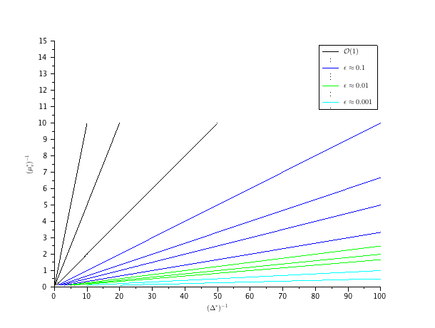
We begin with μvsubscript𝜇𝑣\mu_{v}, and show contour plots as a function of (Δ)1superscriptsuperscriptΔ1(\Delta^{*})^{-1} and of the expected lifespan of the mosquito in Figure 2.
Refer to caption
Figure 2. Scaling for μvsubscript𝜇𝑣\mu_{v} depending on the average lifespan of the vector, and on twice the average infectious time of the host. Although the level curves are just lines, the graph helps to assess the order size of the parameters. A level curve with value L𝐿L was labelled with a certain value of ϵitalic-ϵ\epsilon, if log(Lϵ)[1,0.8]𝐿italic-ϵ10.8\log(L\epsilon)\in[-1,0.8]. This is equivalent to say that L=aϵ1𝐿𝑎superscriptitalic-ϵ1L=a\epsilon^{-1}, a[a0,a1]𝑎subscript𝑎0subscript𝑎1a\in[a_{0},a_{1}], with a00.2subscript𝑎00.2a_{0}\approx 0.2 and a12subscript𝑎12a_{1}\approx 2. Based on the discussion in Section 1.1 and on the values on the level curves, we observe that the range 0.01ϵ0.10.01italic-ϵ0.10.01\leq\epsilon\leq 0.1 seems to match a number of possible scenarios in epidemiological modelling.

With the assumed parameters, we have that

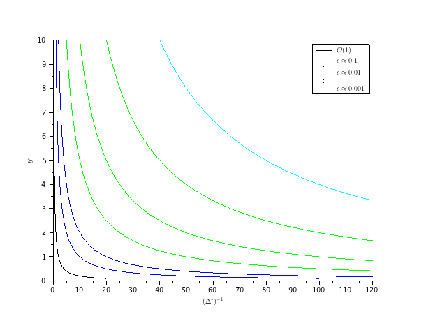
σ=b/2Δandδ=σI.formulae-sequence𝜎superscript𝑏2superscriptΔand𝛿𝜎𝐼\sigma=b^{*}/2\Delta^{*}\quad\text{and}\quad\delta=\sigma I.

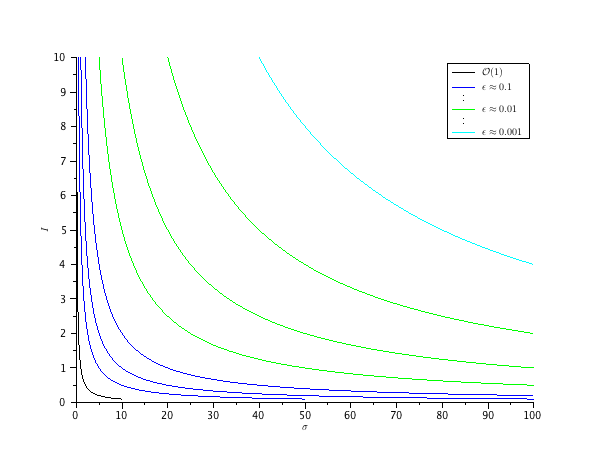
Thus, in Figure 3 we plot the level curves of these expressions. See the corresponding caption for more details, and the caption corresponding to Figure 2 for an explanation about the labelling of the level curves.
Refer to caption
(a)
Refer to caption
(b)
Figure 3. Possible scalings for σ𝜎\sigma and δ𝛿\delta.For the values of bsuperscript𝑏b^{*} that obtained in the literature, the level curves of σ𝜎\sigma are naturally around σ(0.01)1similar-to𝜎superscript0.011\sigma\sim(0.01)^{-1}. Notice that we can easily have δ𝛿\delta of the same order of magnitude than σ𝜎\sigma, in the case of reasonably large infestations. However, for more moderate cases with I0.1𝐼0.1I\approx 0.1, we typycally have δ=𝒪(1)𝛿𝒪1\delta=\mathcal{O}(1). We refer to the discussion in Section 1.1 for a discussion about these values.

The pictures in Figures 2 and 3 suggest both that the proposed regimes are effective, but also that might be a number of other regimes that need to be studied in addition. Additionally, we point out that ϵ=0.01italic-ϵ0.01\epsilon=0.01, seems to be a plausible scaling for Dengue in urban centres—the reader is referred to the discussion in Section 1.1.

3. Global stability analysis

Traditionally, the main focus on study about epidemiological systems as (1) is on global stability issues. In particular a proof of global stability for system (1) using the theory of competitive systems can be found in [19]. More recently, [10] has studied a similar system but with a saturated bilinear incidence. In particular, [10] proved global stability by using a Lyapunov function for the disease-free equilibrium, and using the theory of competitive systems for the endemic equilibrium, whenever it exists. [47] has studied the same system, and provide a Lyapunov proof for the disease-free. The proof presented by [47] for the endemic equilibrium seems to applies only if, in our notation, one has X=1superscript𝑋1X^{*}=1. But in this case, we must necessarily have R0=1subscript𝑅01R_{0}=1. Also a proof using a Lyapunov approach for the disease free equilibrium, and another proof using the theory of competitive systems for the endemic equilibrium can be found in [50].

In what follows, we provide an alternative proof for the global stability of (1) using only Lyapunov functions.

Theorem 1.

Let R0subscript𝑅0R_{0} be defined as above. Then for R01subscript𝑅01R_{0}\leq 1 the disease-free equilibrium is globally asymptotic stable, while for R0>1subscript𝑅01R_{0}>1 the endemic equilibrium is globally asymptotic stable.

Proof.

Although the proof for R01subscript𝑅01R_{0}\leq 1 is available in the literature, as discussed above, we provide it here both for the sake of completeness of presentation, and because the proof given here is somewhat simpler that the available ones.

Suppose R01subscript𝑅01R_{0}\leq 1 and consider the following Lyapunov function

V(X,Y,Z)=XlogX+Y+δμvZ.𝑉𝑋𝑌𝑍𝑋𝑋𝑌𝛿subscript𝜇𝑣𝑍V(X,Y,Z)=X-\log X+Y+\frac{\delta}{\mu_{v}}Z.

Then

V˙=X˙(11X)+Y˙+Z˙˙𝑉˙𝑋11𝑋˙𝑌˙𝑍\dot{V}=\dot{X}\left(1-\frac{1}{X}\right)+\dot{Y}+\dot{Z}

On substituting, we obtain:

V˙=μh(1X)2X(μh+γ)(1R0)YR0ZY,˙𝑉subscript𝜇superscript1𝑋2𝑋subscript𝜇𝛾1subscript𝑅0𝑌subscript𝑅0𝑍𝑌\dot{V}=-\mu_{h}\frac{(1-X)^{2}}{X}-(\mu_{h}+\gamma)(1-R_{0})Y-R_{0}ZY,

which is negative for 0R010subscript𝑅010\leq R_{0}\leq 1, and X,Y,Z𝑋𝑌𝑍X,Y,Z in >03subscriptsuperscript3absent0\mathbb{R}^{3}_{>0}.

For R0>1subscript𝑅01R_{0}>1, let

V(X,Y,Z)=XXlogXX+YYlogYY+δXμv(ZZlogZZ).𝑉𝑋𝑌𝑍𝑋superscript𝑋𝑋superscript𝑋𝑌superscript𝑌𝑌superscript𝑌𝛿superscript𝑋subscript𝜇𝑣𝑍superscript𝑍𝑍superscript𝑍V(X,Y,Z)=X-X^{*}\log\frac{X}{X^{*}}+Y-Y^{*}\log\frac{Y}{Y^{*}}+\frac{\delta X^{*}}{\mu_{v}}\left(Z-Z^{*}\log\frac{Z}{Z^{*}}\right).

Then we have

V˙=˙𝑉absent\displaystyle\dot{V}= X˙(1XX)+Y˙(1YY)+δXμvZ˙(1ZZ)˙𝑋1superscript𝑋𝑋˙𝑌1superscript𝑌𝑌𝛿superscript𝑋subscript𝜇𝑣˙𝑍1superscript𝑍𝑍\displaystyle\dot{X}\left(1-\frac{X^{*}}{X}\right)+\dot{Y}\left(1-\frac{Y^{*}}{Y}\right)+\frac{\delta X^{*}}{\mu_{v}}\dot{Z}\left(1-\frac{Z^{*}}{Z}\right)
=\displaystyle= μh[1+XXXX]+(μh+γ)Y+δXμvZ+σδXμv(1Z)Y+subscript𝜇delimited-[]1superscript𝑋𝑋superscript𝑋𝑋subscript𝜇𝛾superscript𝑌𝛿superscript𝑋subscript𝜇𝑣superscript𝑍limit-from𝜎𝛿superscript𝑋subscript𝜇𝑣1𝑍𝑌\displaystyle\mu_{h}\left[1+X^{*}-X-\frac{X^{*}}{X}\right]+(\mu_{h}+\gamma)Y^{*}+\frac{\delta X^{*}}{\mu_{v}}Z^{*}+\frac{\sigma\delta X^{*}}{\mu_{v}}(1-Z)Y+
δXZYY(μh+γ)YσδXZμv(1Z)YZ𝛿𝑋𝑍superscript𝑌𝑌subscript𝜇𝛾𝑌𝜎𝛿superscript𝑋superscript𝑍subscript𝜇𝑣1𝑍𝑌𝑍\displaystyle\qquad-\delta\frac{XZY^{*}}{Y}-(\mu_{h}+\gamma)Y-\frac{\sigma\delta X^{*}Z^{*}}{\mu_{v}}(1-Z)\frac{Y}{Z}

On using that

(μh+γ)Y=μh(1X)andδXμvZ=μh(1X),formulae-sequencesubscript𝜇𝛾superscript𝑌subscript𝜇1superscript𝑋and𝛿superscript𝑋subscript𝜇𝑣superscript𝑍subscript𝜇1superscript𝑋(\mu_{h}+\gamma)Y^{*}=\mu_{h}(1-X^{*})\quad\text{and}\quad\frac{\delta X^{*}}{\mu_{v}}Z^{*}=\mu_{h}(1-X^{*}),

we arrive at

V˙=˙𝑉absent\displaystyle\dot{V}= μh[3XXXX]+(μh+γ)(R0X(1Z)1)Y+subscript𝜇delimited-[]3superscript𝑋𝑋superscript𝑋𝑋limit-fromsubscript𝜇𝛾subscript𝑅0superscript𝑋1superscript𝑍1𝑌\displaystyle\mu_{h}\left[3-X^{*}-X-\frac{X^{*}}{X}\right]+(\mu_{h}+\gamma)\left(R_{0}X^{*}(1-Z^{*})-1\right)Y+
+σδXμvY[2ZZZZ]δXZYY.𝜎𝛿superscript𝑋subscript𝜇𝑣𝑌delimited-[]2superscript𝑍𝑍superscript𝑍𝑍𝛿𝑋𝑍superscript𝑌𝑌\displaystyle\qquad+\frac{\sigma\delta X^{*}}{\mu_{v}}Y\left[2Z^{*}-Z-\frac{Z^{*}}{Z}\right]-\frac{\delta XZY^{*}}{Y}.

Since

R0(1Z)=R01+D01+R0D0=1X,subscript𝑅01superscript𝑍subscript𝑅01subscript𝐷01subscript𝑅0subscript𝐷01superscript𝑋R_{0}(1-Z^{*})=R_{0}\frac{1+D_{0}}{1+R_{0}D_{0}}=\frac{1}{X^{*}},

we are left with

V˙=μh[3XXXX]+σδXμvY[2ZZZZ]δXZYY.˙𝑉subscript𝜇delimited-[]3superscript𝑋𝑋superscript𝑋𝑋𝜎𝛿superscript𝑋subscript𝜇𝑣𝑌delimited-[]2superscript𝑍𝑍superscript𝑍𝑍𝛿𝑋𝑍superscript𝑌𝑌\dot{V}=\mu_{h}\left[3-X^{*}-X-\frac{X^{*}}{X}\right]+\frac{\sigma\delta X^{*}}{\mu_{v}}Y\left[2Z^{*}-Z-\frac{Z^{*}}{Z}\right]-\frac{\delta XZY^{*}}{Y}.

Writing

X+XX=X+(X)2X+X(1X)X,𝑋superscript𝑋𝑋𝑋superscriptsuperscript𝑋2𝑋superscript𝑋1superscript𝑋𝑋X+\frac{X^{*}}{X}=X+\frac{(X^{*})^{2}}{X}+\frac{X^{*}(1-X^{*})}{X},

using that

X+(X)2X2X,𝑋superscriptsuperscript𝑋2𝑋2superscript𝑋X+\frac{(X^{*})^{2}}{X}\geq 2X^{*},

and on noticing that a similar calculation holds for the second bracket, we find:

(3) V˙3μh(1X)μh(1X)XXσδXμvZ(1Z)ZYδXZYY.˙𝑉3subscript𝜇1superscript𝑋subscript𝜇1superscript𝑋superscript𝑋𝑋𝜎𝛿superscript𝑋subscript𝜇𝑣superscript𝑍1superscript𝑍𝑍𝑌𝛿𝑋𝑍superscript𝑌𝑌\dot{V}\leq 3\mu_{h}(1-X^{*})-\mu_{h}(1-X^{*})\frac{X^{*}}{X}-\frac{\sigma\delta X^{*}}{\mu_{v}}\frac{Z^{*}(1-Z^{*})}{Z}Y-\frac{\delta XZY^{*}}{Y}.

Let us write

R=μh(1X)XXσδXμvZ(1Z)ZYδXZYY.𝑅subscript𝜇1superscript𝑋superscript𝑋𝑋𝜎𝛿superscript𝑋subscript𝜇𝑣superscript𝑍1superscript𝑍𝑍𝑌𝛿𝑋𝑍superscript𝑌𝑌R=-\mu_{h}(1-X^{*})\frac{X^{*}}{X}-\frac{\sigma\delta X^{*}}{\mu_{v}}\frac{Z^{*}(1-Z^{*})}{Z}Y-\frac{\delta XZY^{*}}{Y}.

By the Arithmetic-Geometric inequality, we have

R𝑅absent\displaystyle R\leq 3[μh(1X)XσδμvXZ(1Z)δY]1/33superscriptdelimited-[]subscript𝜇1superscript𝑋superscript𝑋𝜎𝛿subscript𝜇𝑣superscript𝑋superscript𝑍1superscript𝑍𝛿superscript𝑌13\displaystyle-3\left[\mu_{h}(1-X^{*})X^{*}\frac{\sigma\delta}{\mu_{v}}X^{*}Z^{*}(1-Z^{*})\delta Y^{*}\right]^{1/3}
=3[μh2(1X)3D0XR0(1Z)δ]1/3absent3superscriptdelimited-[]superscriptsubscript𝜇2superscript1superscript𝑋3subscript𝐷0superscript𝑋subscript𝑅01superscript𝑍𝛿13\displaystyle=-3\left[\mu_{h}^{2}(1-X^{*})^{3}D_{0}X^{*}R_{0}(1-Z^{*})\delta\right]^{1/3}
=3(1X)[μh2D0δ]1/3absent31superscript𝑋superscriptdelimited-[]superscriptsubscript𝜇2subscript𝐷0𝛿13\displaystyle=-3(1-X^{*})\left[\mu_{h}^{2}D_{0}\delta\right]^{1/3}
=3(1X)μh.absent31superscript𝑋subscript𝜇\displaystyle=-3(1-X^{*})\mu_{h}.

Hence, we have that

V˙0,˙𝑉0\dot{V}\leq 0,

in >03subscriptsuperscript3absent0\mathbb{R}^{3}_{>0}.

In order to show that the V𝑉V is a strict Lyapunov function, we recall that the inequality in (3) is strict unless X=X𝑋superscript𝑋X=X^{*} and Z=Z𝑍superscript𝑍Z=Z^{*}. However, in this case we have that

R𝑅\displaystyle R =μh(1X)σδXμv(1Z)YδXZYYabsentsubscript𝜇1superscript𝑋𝜎𝛿superscript𝑋subscript𝜇𝑣1superscript𝑍𝑌𝛿superscript𝑋superscript𝑍superscript𝑌𝑌\displaystyle=-\mu_{h}(1-X^{*})-\frac{\sigma\delta X^{*}}{\mu_{v}}(1-Z^{*})Y-\frac{\delta X^{*}Z^{*}Y^{*}}{Y}
=μh(1X)(μh+γ)YδD0(1X)YYabsentsubscript𝜇1superscript𝑋subscript𝜇𝛾𝑌𝛿subscript𝐷01superscript𝑋superscript𝑌𝑌\displaystyle=-\mu_{h}(1-X^{*})-(\mu_{h}+\gamma)Y-\delta D_{0}(1-X^{*})\frac{Y^{*}}{Y}
=μh(1X)[1+YY+YY]absentsubscript𝜇1superscript𝑋delimited-[]1𝑌superscript𝑌superscript𝑌𝑌\displaystyle=-\mu_{h}(1-X^{*})\left[1+\frac{Y}{Y^{*}}+\frac{Y^{*}}{Y}\right]

Since

YY+YY2,𝑌superscript𝑌superscript𝑌𝑌2\frac{Y}{Y^{*}}+\frac{Y^{*}}{Y}\geq 2,

with equality only when Y=Y𝑌superscript𝑌Y=Y^{*}, we conclude that R<μh(1X)𝑅subscript𝜇1superscript𝑋R<-\mu_{h}(1-X^{*}), except on (X,Y,Z)=(X,Y,Z)𝑋𝑌𝑍superscript𝑋superscript𝑌superscript𝑍(X,Y,Z)=(X^{*},Y^{*},Z^{*}) where we have equality. Therefore, we have V˙<0˙𝑉0\dot{V}<0 in >03subscriptsuperscript3absent0\mathbb{R}^{3}_{>0}, except in the endemic equilibrium.     square-intersection\sqcapsquare-union\sqcup

square-intersection\sqcapsquare-union\sqcup

4. The fast vector dynamics

As discussed above, we want to describe the dynamics of system (2), when we have:

σ=σ¯ϵ1andμv=μ¯vϵ1,0<ϵ1,formulae-sequence𝜎¯𝜎superscriptitalic-ϵ1andformulae-sequencesubscript𝜇𝑣subscript¯𝜇𝑣superscriptitalic-ϵ10italic-ϵmuch-less-than1\sigma=\bar{\sigma}\epsilon^{-1}\quad\text{and}\quad\mu_{v}=\bar{\mu}_{v}\epsilon^{-1},\quad 0<\epsilon\ll 1,

while all other parameters are of order one.

Direct substitution in (2) lead us to the following initial value problem:

(4) {X˙=μh(1X)δXZY˙=δXZ(μh+γ)YϵZ˙=σ¯(1Z)Yμ¯vZcases˙𝑋subscript𝜇1𝑋𝛿𝑋𝑍˙𝑌𝛿𝑋𝑍subscript𝜇𝛾𝑌italic-ϵ˙𝑍¯𝜎1𝑍𝑌subscript¯𝜇𝑣𝑍\left\{\begin{array}[]{rcl}\dot{X}&=&\mu_{h}(1-X)-\delta XZ\\ \dot{Y}&=&\delta XZ-(\mu_{h}+\gamma)Y\\ \epsilon\dot{Z}&=&\bar{\sigma}(1-Z)Y-\bar{\mu}_{v}Z\end{array}\right.

subject to the initial condition

X(0)=X0,Y(0)=Y0andZ(0)=Z0.formulae-sequence𝑋0subscript𝑋0formulae-sequence𝑌0subscript𝑌0and𝑍0subscript𝑍0X(0)=X_{0},\quad Y(0)=Y_{0}\quad\text{and}\quad Z(0)=Z_{0}.

On a formal basis, since we already know that the dynamics of (2) always converges to an equilibrium, we expect that the right hand side of the last equation balances out, leaving Z˙0˙𝑍0\dot{Z}\approx 0, i.e, that the vector population is nearly in equilibrium. Under these hypothesis, we obtain the following system:

(5) {X˙=μh(1X)δσXYσY+μvY˙=δσXYσY+μv(μh+γ)YZ˙=0cases˙𝑋subscript𝜇1𝑋𝛿𝜎𝑋𝑌𝜎𝑌subscript𝜇𝑣˙𝑌𝛿𝜎𝑋𝑌𝜎𝑌subscript𝜇𝑣subscript𝜇𝛾𝑌˙𝑍0\left\{\begin{array}[]{rcl}\dot{X}&=&\mu_{h}(1-X)-\delta\frac{\sigma XY}{\sigma Y+\mu_{v}}\\ \dot{Y}&=&\delta\frac{\sigma XY}{\sigma Y+\mu_{v}}-(\mu_{h}+\gamma)Y\\ \dot{Z}&=&0\end{array}\right.

Notice that system (5) can be seen as a SIR system with a modified, rational, incidence rate. While the above derivation is heuristic, we now show that it can obtained from a consistent multiscale asymptotic expansion and, moreover, that such an expansion can be rigorously justified.

4.1. Asymptotic expansion

Let

ϵτ=t.italic-ϵ𝜏𝑡\epsilon\tau=t.

Then, we seek a composite expansion of the form

X𝑋\displaystyle X =X0(t)+𝒪(ϵ)absentsuperscript𝑋0𝑡𝒪italic-ϵ\displaystyle=X^{0}(t)+\mathcal{O}(\epsilon)
Y𝑌\displaystyle Y =Y0(t)+𝒪(ϵ)andabsentsuperscript𝑌0𝑡𝒪italic-ϵand\displaystyle=Y^{0}(t)+\mathcal{O}(\epsilon)\quad\text{and}
Z𝑍\displaystyle Z =Z0(t)+Z^0(τ)+𝒪(ϵ),absentsuperscript𝑍0𝑡superscript^𝑍0𝜏𝒪italic-ϵ\displaystyle=Z^{0}(t)+\hat{Z}^{0}(\tau)+\mathcal{O}(\epsilon),

where

limτZ^0(τ)=0.subscript𝜏superscript^𝑍0𝜏0\lim_{\tau\to\infty}\hat{Z}^{0}(\tau)=0.

On substituting the proposed expansion in (4), we obtain to leading order the following differential-algebraic system:

Xt0=subscriptsuperscript𝑋0𝑡absent\displaystyle X^{0}_{t}= μh(1X0)δX0Z0subscript𝜇1superscript𝑋0𝛿superscript𝑋0superscript𝑍0\displaystyle\mu_{h}(1-X^{0})-\delta X^{0}Z^{0}
Yt0=subscriptsuperscript𝑌0𝑡absent\displaystyle Y^{0}_{t}= δX0Z0(μh+γ)Y0𝛿superscript𝑋0superscript𝑍0subscript𝜇𝛾superscript𝑌0\displaystyle\delta X^{0}Z^{0}-(\mu_{h}+\gamma)Y^{0}
0=0absent\displaystyle 0= σ¯(1Z0)Y0μ¯vZ0.¯𝜎1superscript𝑍0superscript𝑌0subscript¯𝜇𝑣superscript𝑍0\displaystyle\bar{\sigma}(1-Z^{0})Y^{0}-\bar{\mu}_{v}Z^{0}.

This yields

(6) Z0(t)=σ¯Y0(t)σ¯Y0(t)+μ¯v.superscript𝑍0𝑡¯𝜎superscript𝑌0𝑡¯𝜎superscript𝑌0𝑡subscript¯𝜇𝑣Z^{0}(t)=\frac{\bar{\sigma}Y^{0}(t)}{\bar{\sigma}Y^{0}(t)+\bar{\mu}_{v}}.

and hence, we obtain the system:

(7) {Xt0=μh(1X0)δσ¯X0Y0σ¯Y0+μ¯vYt0=δσ¯X0Y0σ¯Y0+μ¯v(μh+γ)Y0casessubscriptsuperscript𝑋0𝑡subscript𝜇1superscript𝑋0𝛿¯𝜎superscript𝑋0superscript𝑌0¯𝜎superscript𝑌0subscript¯𝜇𝑣subscriptsuperscript𝑌0𝑡𝛿¯𝜎superscript𝑋0superscript𝑌0¯𝜎superscript𝑌0subscript¯𝜇𝑣subscript𝜇𝛾superscript𝑌0\left\{\begin{array}[]{rcl}X^{0}_{t}&=&\mu_{h}(1-X^{0})-\delta\frac{\bar{\sigma}X^{0}Y^{0}}{\bar{\sigma}Y^{0}+\bar{\mu}_{v}}\\ Y^{0}_{t}&=&\delta\frac{\bar{\sigma}X^{0}Y^{0}}{\bar{\sigma}Y^{0}+\bar{\mu}_{v}}-(\mu_{h}+\gamma)Y^{0}\\ \end{array}\right.

with initial condition X0(0)=X0superscript𝑋00subscript𝑋0X^{0}(0)=X_{0} and Y0(0)=Y0superscript𝑌00subscript𝑌0Y^{0}(0)=Y_{0}.

Notice that, in general, we have Z0(0)Z0superscript𝑍00subscript𝑍0Z^{0}(0)\not=Z_{0}. Such a mismatch in the initial condition, should be corrected by Z^0superscript^𝑍0\hat{Z}^{0}. Thus, Z^0superscript^𝑍0\hat{Z}^{0} should satisfy both Z0(0)=Z0Z0(0)^^superscript𝑍00subscript𝑍0superscript𝑍00\hat{Z^{0}(0)=Z_{0}-Z^{0}(0)} (it adjusts for the correct initial condition) and Z^0(τ)0superscript^𝑍0𝜏0\hat{Z}^{0}(\tau)\to 0, as τ𝜏\tau\to\infty (it has a local character). In order to solve for Z^0superscript^𝑍0\hat{Z}^{0}, we first observe that

X0(t)=X0(ϵτ)=X0(0)+ϵτXt0(0)+𝒪(ϵ2),superscript𝑋0𝑡superscript𝑋0italic-ϵ𝜏superscript𝑋00italic-ϵ𝜏subscriptsuperscript𝑋0𝑡0𝒪superscriptitalic-ϵ2X^{0}(t)=X^{0}(\epsilon\tau)=X^{0}(0)+\epsilon\tau X^{0}_{t}(0)+\mathcal{O}(\epsilon^{2}),

with similar expansions for Y0(t)superscript𝑌0𝑡Y^{0}(t) and Z0(t)superscript𝑍0𝑡Z^{0}(t).

Hence, we find that Z^0superscript^𝑍0\hat{Z}^{0} satisfies

Z^τ0=(σ¯Y0+μ¯v)Z^0,subscriptsuperscript^𝑍0𝜏¯𝜎subscript𝑌0subscript¯𝜇𝑣superscript^𝑍0\hat{Z}^{0}_{\tau}=-(\bar{\sigma}Y_{0}+\bar{\mu}_{v})\hat{Z}^{0},

i.e

(8) Z^0(τ)=(Z0σ¯Y0σ¯Y0+μ¯v)e(σ¯Y0+μ¯v)τ.superscript^𝑍0𝜏subscript𝑍0¯𝜎subscript𝑌0¯𝜎subscript𝑌0subscript¯𝜇𝑣superscripte¯𝜎subscript𝑌0subscript¯𝜇𝑣𝜏\hat{Z}^{0}(\tau)=\left(Z_{0}-\frac{\bar{\sigma}Y_{0}}{\bar{\sigma}Y_{0}+\bar{\mu}_{v}}\right)\mathrm{e}^{-(\bar{\sigma}Y_{0}+\bar{\mu}_{v})\tau}.

4.2. Global stability analysis of the asymptotic system

Before we can assert the quality of the approximation provided by (6), (7) and (8), we need a better understanding of the dynamics of the reduced system. We begin with the following basic result:

Proposition 1.

Let

𝒮={(X0,Y0)2|X0+Y01,X0,Y00}.𝒮conditional-setsuperscript𝑋0superscript𝑌0superscript2formulae-sequencesuperscript𝑋0superscript𝑌01superscript𝑋0superscript𝑌00\mathcal{S}=\{(X^{0},Y^{0})\in\mathbb{R}^{2}\,|\,X^{0}+Y^{0}\leq 1,\quad X^{0},Y^{0}\geq 0\}.

Then 𝒮𝒮\mathcal{S} is invariant by the flow of (7). In particular, the corresponding solutions are global in time.

Proof.

Since Y0=0superscript𝑌00Y^{0}=0 is an invariant set, a solution with Y00superscript𝑌00Y^{0}\geq 0 at any time, will remain this property. Also, when X0=0superscript𝑋00X^{0}=0, the flow points inside 𝒮𝒮\mathcal{S}. Thus, for an initial condition in 𝒮𝒮\mathcal{S}, we also have X00superscript𝑋00X^{0}\geq 0. Finally, (X0+Y0)t0subscriptsuperscript𝑋0superscript𝑌0𝑡0(X^{0}+Y^{0})_{t}\leq 0.     square-intersection\sqcapsquare-union\sqcup

square-intersection\sqcapsquare-union\sqcup

System (7) has two equilibrium points in the positive quadrant:

  1. (1)

    X=1subscript𝑋1X_{*}=1, Y=0subscript𝑌0Y_{*}=0.

  2. (2)
    X=(μh+γ)μ¯v+νhσ¯(μh+δ)σ¯andY=δμnσ¯(μh2+γμh)μ¯vμh2+(γ+δ)h+δγ)σ¯.X_{*}=\frac{(\mu_{h}+\gamma)\bar{\mu}_{v}+\nu_{h}\bar{\sigma}}{(\mu_{h}+\delta)\bar{\sigma}}\quad\text{and}\quad Y_{*}=\frac{\delta\mu_{n}\bar{\sigma}-(\mu_{h}^{2}+\gamma\mu_{h})\bar{\mu}_{v}}{\mu_{h}^{2}+(\gamma+\delta)h+\delta\gamma)\bar{\sigma}}.
Remark 1.

Notice that X=Xsubscript𝑋superscript𝑋X_{*}=X^{*} and Y=Ysubscript𝑌superscript𝑌Y_{*}=Y^{*}. Thus the equilibria of (7) correspond to the projections in the XY𝑋𝑌XY plane of the equilibria of (2). Notice also that

Z=σ¯Yσ¯Y+μ¯v=Z.subscript𝑍¯𝜎subscript𝑌¯𝜎subscript𝑌subscript¯𝜇𝑣superscript𝑍Z_{*}=\frac{\bar{\sigma}Y_{*}}{\bar{\sigma}Y_{*}+\bar{\mu}_{v}}=Z^{*}.

The next result shows that the dynamics of systems (11) and (7) are qualitatively equivalent, in the sense that either both end up in the disease free equilibrium or in the endemic one.

Theorem 2.

Let

R¯0=δσ¯μ¯v(νh+γ)subscript¯𝑅0𝛿¯𝜎subscript¯𝜇𝑣subscript𝜈𝛾\bar{R}_{0}=\frac{\delta\bar{\sigma}}{\bar{\mu}_{v}(\nu_{h}+\gamma)}

Then R¯0=R0subscript¯𝑅0subscript𝑅0\bar{R}_{0}=R_{0}, and for R01subscript𝑅01R_{0}\leq 1 the disease free equilibrium is globally asymptotically stable. For R0>1subscript𝑅01R_{0}>1, the endemic equilibrium is globally asymptotically stable.

Proof.

The assertion about R0subscript𝑅0R_{0} is clear. For the global stability, let

F(Y0)=σ¯Y0+μ¯vY0𝐹superscript𝑌0¯𝜎superscript𝑌0subscript¯𝜇𝑣superscript𝑌0F(Y^{0})=\frac{\bar{\sigma}Y^{0}+\bar{\mu}_{v}}{Y^{0}}

Then F𝐹F is a Dulac function for the system (7) in compact subsets of 𝒮𝒮\mathcal{S} that do not intersect the X0superscript𝑋0X^{0} axis, since we have:

X0[μh(1X0)F(Y0)δX0]+Y0[δX0(μh+γ)(σ¯Y0+μv)=μhF(Y0)δσ¯(μh+γ)<0.\partial_{X^{0}}[\mu_{h}(1-X^{0})F(Y^{0})-\delta X^{0}]+\partial_{Y^{0}}[\delta X^{0}-(\mu_{h}+\gamma)(\bar{\sigma}Y^{0}+\mu_{v})=-\mu_{h}F(Y^{0})-\delta-\bar{\sigma}(\mu_{h}+\gamma)<0.

Thus, the system cannot have a closed orbit in the interior of 𝒮𝒮\mathcal{S}. For R01subscript𝑅01R_{0}\leq 1, the only equilibrium in 𝒮𝒮\mathcal{S} is (1,0)10(1,0). Thus all orbits must converge to this equilibrium point.

The linearisation of (7) is

(X¯0Y¯0)T=(μhδσ¯Y0σ¯Y0+μ¯vσ¯δX0μ¯v(σ¯Y0+μ¯v)2δσ¯Y0σ¯Y0+μ¯vσ¯δX0μ¯v(σ¯Y0+μ¯v)2μhγ)(X¯0Y¯0)subscriptmatrixsuperscript¯𝑋0superscript¯𝑌0𝑇matrixsubscript𝜇𝛿¯𝜎superscript𝑌0¯𝜎superscript𝑌0subscript¯𝜇𝑣¯𝜎𝛿superscript𝑋0subscript¯𝜇𝑣superscript¯𝜎superscript𝑌0subscript¯𝜇𝑣2𝛿¯𝜎superscript𝑌0¯𝜎superscript𝑌0subscript¯𝜇𝑣¯𝜎𝛿superscript𝑋0subscript¯𝜇𝑣superscript¯𝜎superscript𝑌0subscript¯𝜇𝑣2subscript𝜇𝛾matrixsuperscript¯𝑋0superscript¯𝑌0\begin{pmatrix}\bar{X}^{0}\\ \bar{Y}^{0}\end{pmatrix}_{T}=\begin{pmatrix}-\mu_{h}-\delta\frac{\bar{\sigma}Y^{0}}{\bar{\sigma}Y^{0}+\bar{\mu}_{v}}&-\bar{\sigma}\delta X^{0}\frac{\bar{\mu}_{v}}{(\bar{\sigma}Y^{0}+\bar{\mu}_{v})^{2}}\\ \delta\frac{\bar{\sigma}Y^{0}}{\bar{\sigma}Y^{0}+\bar{\mu}_{v}}&\bar{\sigma}\delta X^{0}\frac{\bar{\mu}_{v}}{(\bar{\sigma}Y^{0}+\bar{\mu}_{v})^{2}}-\mu_{h}-\gamma\\ \end{pmatrix}\begin{pmatrix}\bar{X}^{0}\\ \bar{Y}^{0}\end{pmatrix}

For the disease free equilibrium, the eigenvalues of the Jacobian are μhsubscript𝜇-\mu_{h} and (μh+γ)(R01)subscript𝜇𝛾subscript𝑅01(\mu_{h}+\gamma)(R_{0}-1). Thus, the disease free equilibrium is a locally asymptotically stable node for R0<1subscript𝑅01R_{0}<1, and a saddle for R0>1subscript𝑅01R_{0}>1. In the latter case, the unique orbit that approaches the disease free equilibrium is easily shown to be the intersection of 𝒮𝒮\mathcal{S} with Y0=0superscript𝑌00Y^{0}=0. Thus, all the other orbits must approach the endemic equilibrium.     square-intersection\sqcapsquare-union\sqcup

square-intersection\sqcapsquare-union\sqcup

4.3. Asymptotic convergence and numerical results

The asymptotic expansions derived in 4.1 can be shown to be indeed asymptotic. The ideas used here are similar to the ones used to formalise Kinetic Menton’s theory—cf. [36] and references therein for instance. In particular, we have the following:

Theorem 3.

Let 𝔛ϵ(t)=(X(t),Y(t),Z(t))superscript𝔛italic-ϵ𝑡𝑋𝑡𝑌𝑡𝑍𝑡\mathfrak{X}^{\epsilon}(t)=(X(t),Y(t),Z(t)) and 𝔛0(t,τ)=(X0(t),Y0(t),Z0(t)+Z^0(τ))superscript𝔛0𝑡𝜏superscript𝑋0𝑡superscript𝑌0𝑡superscript𝑍0𝑡superscript^𝑍0𝜏\mathfrak{X}^{0}(t,\tau)=(X^{0}(t),Y^{0}(t),Z^{0}(t)+\hat{Z}^{0}(\tau)). Denote the uniform norm in [0,)0[0,\infty) by .\|.\|_{\infty}. Then, for sufficient small ϵ>0italic-ϵ0\epsilon>0, there exists a constant C>0𝐶0C>0, independent of ϵitalic-ϵ\epsilon, such that

𝔛𝔛0Cϵ.subscriptnorm𝔛superscript𝔛0𝐶italic-ϵ\|\mathfrak{X}-\mathfrak{X}^{0}\|_{\infty}\leq C\epsilon.

Moreover, let hfX0(t)=(X0(t),Y0(t),Z0(t))𝑓superscript𝑋0𝑡superscript𝑋0𝑡superscript𝑌0𝑡superscript𝑍0𝑡\\ hfX^{0}(t)=(X^{0}(t),Y^{0}(t),Z^{0}(t)). Then there are constants C1,C2>0subscript𝐶1subscript𝐶20C_{1},C_{2}>0 such that, for t>C1ϵ𝑡subscript𝐶1italic-ϵt>C_{1}\epsilon, we have

𝔛ϵ(t)𝔛^0(t)C2ϵ.normsuperscript𝔛italic-ϵ𝑡superscript^𝔛0𝑡subscript𝐶2italic-ϵ\|\mathfrak{X}^{\epsilon}(t)-\hat{\mathfrak{X}}^{0}(t)\|\leq C_{2}\epsilon.

The proof of Theorem 3 is given in Appendix A.

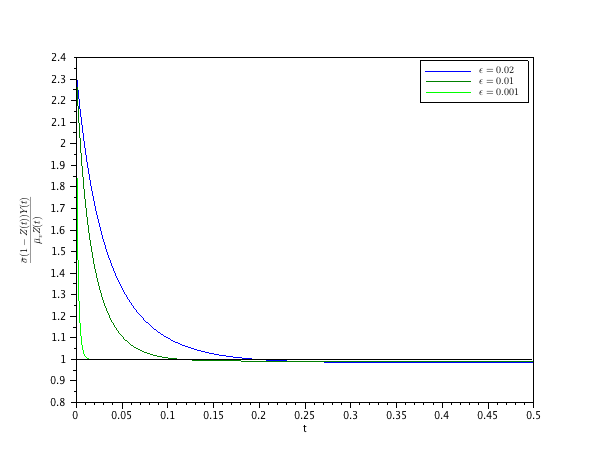
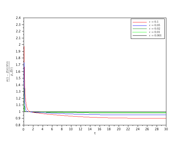
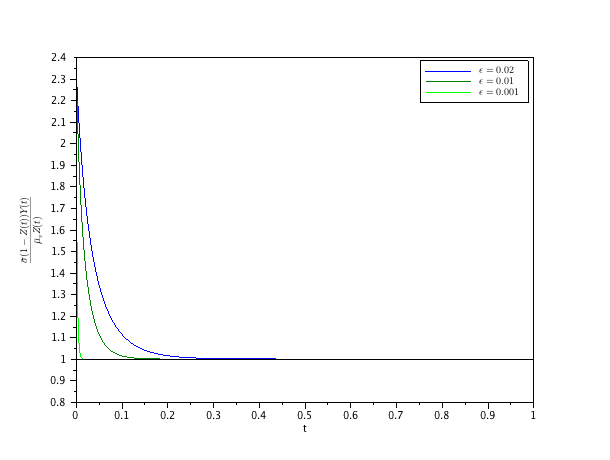
We now present some numerical illustrations. We first observe that the hallmark of the Fast Vector Dynamics is that

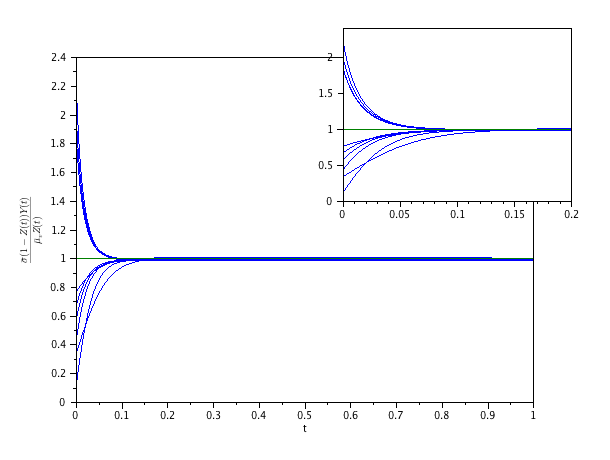
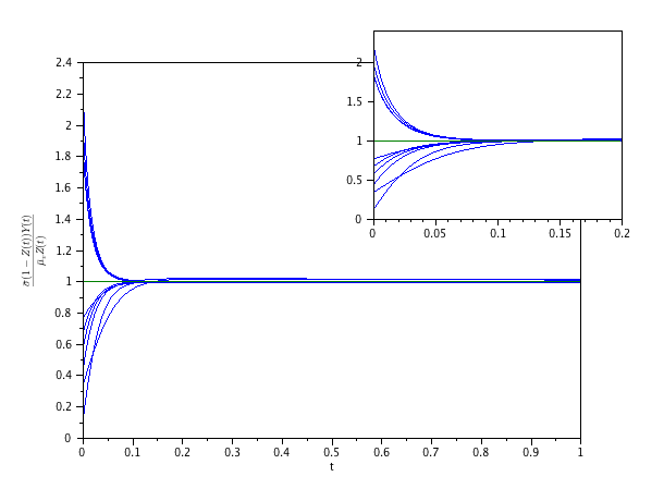
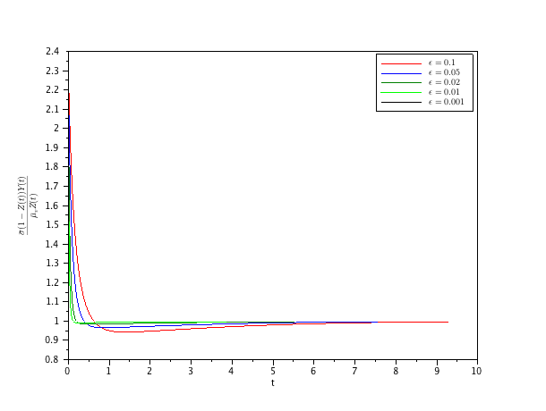
(9) σ¯(1Z(t))Y(t)μ¯vZ(t)=1.¯𝜎1𝑍𝑡𝑌𝑡subscript¯𝜇𝑣𝑍𝑡1\frac{\bar{\sigma}(1-Z(t))Y(t)}{\bar{\mu}_{v}Z(t)}=1.

In Figures 4 and 5 we check performance of the approximation in terms of (9) for two different parameter sets: the first one has μh=0.4subscript𝜇0.4\mu_{h}=0.4, γ=0.25𝛾0.25\gamma=0.25, δ=0.5𝛿0.5\delta=0.5, μ¯v=0.2subscript¯𝜇𝑣0.2\bar{\mu}_{v}=0.2, and σ¯=0.5¯𝜎0.5\bar{\sigma}=0.5; the second set has μh=0.0005subscript𝜇0.0005\mu_{h}=0.0005, with the other parameters values equal to the first set. Two verifications are performed: in Figure 4, we verify the performance of the approximation with a fixed small ϵitalic-ϵ\epsilon, but with a number of different initial conditions; in Figure 5, we now fix an initial condition, but have a number of different values of ϵitalic-ϵ\epsilon.

Refer to caption
(a) Parameter set 1
Refer to caption
(b) Parameter set 2
Figure 4. We show how the ratio in (9) is attained for the set of parameters described in the text. In these numerical experiments we have ϵ=0.01italic-ϵ0.01\epsilon=0.01, and a set of ten initial conditions that was randomically generated—but kept constant for the two figures. For both sets, the endemic equilibrium is globablly stable, but typically these equilibria are attained arround time t=10𝑡10t=10 for the first parameter set, and about t=700𝑡700t=700 for the second set. Hence, convergence to (9) at earlier times, as shown in the graphs, is not a consequence of convergence to equilibrium.
Refer to caption
(a) Parameter set 1
Refer to caption
(b) Parameter set 1 — detail
Refer to caption
(c) Parameter set 2
Refer to caption
(d) Parameter set 2 — detail
Figure 5. The dependence of the ratio given by (9) for a fixed initial condition as a function of the gauge parameter ϵitalic-ϵ\epsilon. For the two parameter sets, the results are similar in the sense that for ϵ0.02italic-ϵ0.02\epsilon\leq 0.02, the approximation seems to perform very efficiently. .

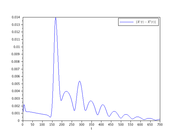
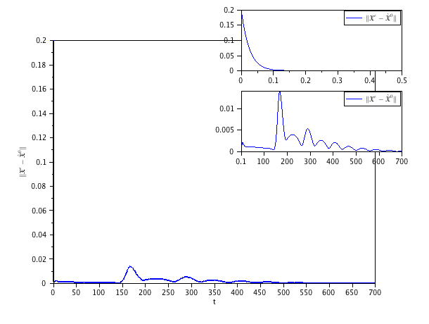
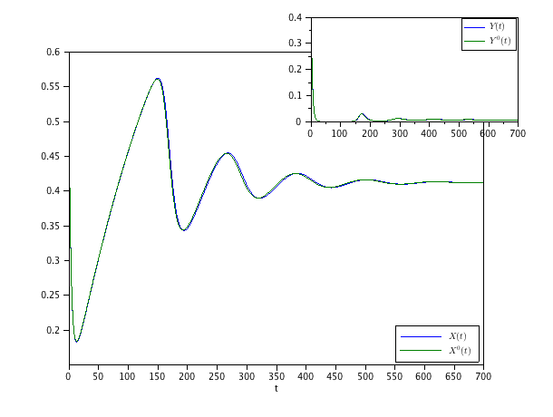
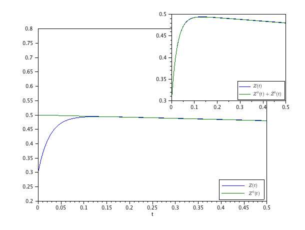
We now present further results for a third parameter set in Figure 6. There we compare the full model with the asymptotic model. As expected, the approximation of X(t)𝑋𝑡X(t) by X0(t)superscript𝑋0𝑡X^{0}(t) and of Y(t)𝑌𝑡Y(t) by Y0(t)superscript𝑌0𝑡Y^{0}(t) are indeed uniform for all time, while the approximation of Z(t)𝑍𝑡Z(t) by Z0(t)superscript𝑍0𝑡Z^{0}(t) fail to be uniform in an initial layer. Notice also that such non-uniform behaviour is suppressed by including the corrector term in the initial layer. This parameter set has μh=0.005subscript𝜇0.005\mu_{h}=0.005, γ=0.4𝛾0.4\gamma=0.4, δ=0.4𝛿0.4\delta=0.4, μ¯v=0.2subscript¯𝜇𝑣0.2\bar{\mu}_{v}=0.2, and σ¯=0.5¯𝜎0.5\bar{\sigma}=0.5.

Refer to caption
(a)
Refer to caption
(b)
Refer to caption
(c)
Refer to caption
(d)
Figure 6. In (a) we show that the error in the composite approximation stays well within the expected bounds. The non uniformity within an initial transition layer is first seen in (b) when compare the norms of the leading-order terms without the transition corrector in Z𝑍Z. The insets show that larger discrepancy indeed comes from the lack of the corrector Z^^𝑍\hat{Z}. Such non uniformity is also clearly depicted in (d), with the inset showing the efectiveness of the composite approximation for the Z𝑍Z component, while (c) shows that the leading order for X𝑋X (and Y𝑌Y in the inset)—without any correctors—work also effectively well.
Refer to caption
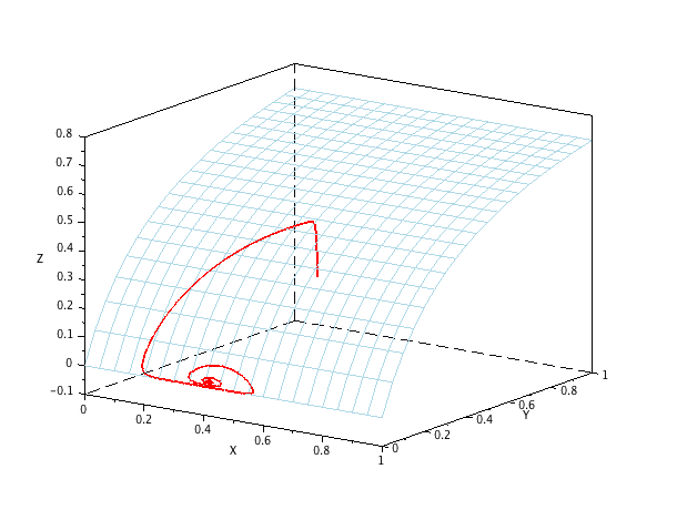
Figure 7. The slow manifold dynamics. As already indicated by the Figures 4 and 5, we also have that the most of the trajectory remains asymptotically close to the manifold. Parameter values are as in figure 6

5. The fast host dynamics

Analogous to the previous case, we now assume that the dynamics of the host is much faster than the dynamics of the vector. In this case, one might expect that the host population is nearly in equilibrium. Hence, we should have X˙0˙𝑋0\dot{X}\approx 0 and Y˙0˙𝑌0\dot{Y}\approx 0, i.e, we should have the system

(10) {0=μh(1X)δσXYσY+μv0=δσXYσY+μv(μh+γ)YZ˙=σ(1Z)YμvZcases0subscript𝜇1𝑋𝛿𝜎𝑋𝑌𝜎𝑌subscript𝜇𝑣0𝛿𝜎𝑋𝑌𝜎𝑌subscript𝜇𝑣subscript𝜇𝛾𝑌˙𝑍𝜎1𝑍𝑌subscript𝜇𝑣𝑍\left\{\begin{array}[]{rcl}0&=&\mu_{h}(1-X)-\delta\frac{\sigma XY}{\sigma Y+\mu_{v}}\\ 0&=&\delta\frac{\sigma XY}{\sigma Y+\mu_{v}}-(\mu_{h}+\gamma)Y\\ \dot{Z}&=&\sigma(1-Z)Y-\mu_{v}Z\end{array}\right.

Equation (10) is a SI system for the vector, with a modified incidence rate.

In order to justify system (10), we assume that

δ=δ¯ϵ1,μh=μ¯hϵ1andγ=γ¯ϵ1.formulae-sequence𝛿¯𝛿superscriptitalic-ϵ1formulae-sequencesubscript𝜇subscript¯𝜇superscriptitalic-ϵ1and𝛾¯𝛾superscriptitalic-ϵ1\delta=\bar{\delta}\epsilon^{-1},\quad\mu_{h}=\bar{\mu}_{h}\epsilon^{-1}\quad\text{and}\quad\gamma=\bar{\gamma}\epsilon^{-1}.

Thus, we are interested in solving

(11) {ϵX˙=μ¯h(1X)δ¯XZϵY˙=δ¯XZ(μ¯h+γ¯)YZ˙=σ(1Z)YμvZcasesitalic-ϵ˙𝑋subscript¯𝜇1𝑋¯𝛿𝑋𝑍italic-ϵ˙𝑌¯𝛿𝑋𝑍subscript¯𝜇¯𝛾𝑌˙𝑍𝜎1𝑍𝑌subscript𝜇𝑣𝑍\left\{\begin{array}[]{rcl}\epsilon\dot{X}&=&\bar{\mu}_{h}(1-X)-\bar{\delta}XZ\\ \epsilon\dot{Y}&=&\bar{\delta}XZ-(\bar{\mu}_{h}+\bar{\gamma})Y\\ \dot{Z}&=&\sigma(1-Z)Y-\mu_{v}Z\end{array}\right.

subject to the initial condition

X(0)=X0,Y(0)=Y0andZ(0)=Z0.formulae-sequence𝑋0subscript𝑋0formulae-sequence𝑌0subscript𝑌0and𝑍0subscript𝑍0X(0)=X_{0},\quad Y(0)=Y_{0}\quad\text{and}\quad Z(0)=Z_{0}.

In what follows, we formally derive the leading order asymptotic expansion and provide a global analysis together with some numerical results. The proof that this expansion is asymptotic is very similar to the Fast Vector Dynamics regime, and hence it is omitted.

5.1. Asymptotic expansion

As before, we let ϵτ=titalic-ϵ𝜏𝑡\epsilon\tau=t. The asymptotic expansion now take the following form:

X(t)𝑋𝑡\displaystyle X(t) =X0(t)+X^0(τ)+𝒪(ϵ),absentsuperscript𝑋0𝑡superscript^𝑋0𝜏𝒪italic-ϵ\displaystyle=X^{0}(t)+\hat{X}^{0}(\tau)+\mathcal{O}(\epsilon),
Y(t)𝑌𝑡\displaystyle Y(t) =Y0(t)+Y^0(τ)+𝒪(ϵ),absentsuperscript𝑌0𝑡superscript^𝑌0𝜏𝒪italic-ϵ\displaystyle=Y^{0}(t)+\hat{Y}^{0}(\tau)+\mathcal{O}(\epsilon),
Z(t)𝑍𝑡\displaystyle Z(t) =Z0(t)+𝒪(ϵ).absentsuperscript𝑍0𝑡𝒪italic-ϵ\displaystyle=Z^{0}(t)+\mathcal{O}(\epsilon).

Here, we also have

limτ(X^0(τ),Y^0(τ)=0.\lim_{\tau\to\infty}(\hat{X}^{0}(\tau),\hat{Y}^{0}(\tau)=0.

At leading order, we have

00\displaystyle 0 =μ¯h(1X0)δ¯X0Z0absentsubscript¯𝜇1superscript𝑋0¯𝛿superscript𝑋0superscript𝑍0\displaystyle=\bar{\mu}_{h}(1-X^{0})-\bar{\delta}X^{0}Z^{0}
00\displaystyle 0 =δ¯X0Z0(μ¯h+γ¯)Y0absent¯𝛿superscript𝑋0superscript𝑍0subscript¯𝜇¯𝛾superscript𝑌0\displaystyle=\bar{\delta}X^{0}Z^{0}-(\bar{\mu}_{h}+\bar{\gamma})Y^{0}
Zt0subscriptsuperscript𝑍0𝑡\displaystyle Z^{0}_{t} =σ(1Z0)Y0μvZ0absent𝜎1superscript𝑍0superscript𝑌0subscript𝜇𝑣superscript𝑍0\displaystyle=\sigma(1-Z^{0})Y^{0}-\mu_{v}Z^{0}

We solve for X0superscript𝑋0X^{0} and Y0superscript𝑌0Y^{0} obtaining

X0=μ¯hδ¯Z+μ¯handY0=δ¯μ¯hμ¯h+γ¯Z0δ¯Z0+μ¯h.formulae-sequencesuperscript𝑋0subscript¯𝜇¯𝛿𝑍subscript¯𝜇andsuperscript𝑌0¯𝛿subscript¯𝜇subscript¯𝜇¯𝛾superscript𝑍0¯𝛿superscript𝑍0subscript¯𝜇X^{0}=\frac{\bar{\mu}_{h}}{\bar{\delta}Z+\bar{\mu}_{h}}\quad\text{and}\quad Y^{0}=\frac{\bar{\delta}\bar{\mu}_{h}}{\bar{\mu}_{h}+\bar{\gamma}}\frac{Z^{0}}{\bar{\delta}Z^{0}+\bar{\mu}_{h}}.

Thus the last equation becomes

Zt0=μvZ0(R0D01Z0Z0+D01).subscriptsuperscript𝑍0𝑡subscript𝜇𝑣superscript𝑍0subscript𝑅0subscript𝐷01superscript𝑍0superscript𝑍0subscript𝐷01Z^{0}_{t}=\mu_{v}Z^{0}\left(R_{0}D_{0}\frac{1-Z^{0}}{Z^{0}+D_{0}}-1\right).

Also, we write

Z0(t)=Z0(ϵτ)=Z0(0)+ϵτZ0(0)+𝒪(ϵ2τ2),superscript𝑍0𝑡superscript𝑍0italic-ϵ𝜏superscript𝑍00italic-ϵ𝜏superscript𝑍00𝒪superscriptitalic-ϵ2superscript𝜏2Z^{0}(t)=Z^{0}(\epsilon\tau)=Z^{0}(0)+\epsilon\tau Z^{0}(0)+\mathcal{O}(\epsilon^{2}\tau^{2}),

hence, since Z0(0)=Z0superscript𝑍00subscript𝑍0Z^{0}(0)=Z_{0}, we obtain

X^τ0subscriptsuperscript^𝑋0𝜏\displaystyle\hat{X}^{0}_{\tau} =μ¯hX^0δ¯X^0Z0absentsubscript¯𝜇superscript^𝑋0¯𝛿superscript^𝑋0subscript𝑍0\displaystyle=\bar{\mu}_{h}\hat{X}^{0}-\bar{\delta}\hat{X}^{0}Z_{0}
Y^τ0subscriptsuperscript^𝑌0𝜏\displaystyle\hat{Y}^{0}_{\tau} =δ¯X^0Z0=(γ¯+μ¯h)Y^0absent¯𝛿superscript^𝑋0subscript𝑍0¯𝛾subscript¯𝜇superscript^𝑌0\displaystyle=\bar{\delta}\hat{X}^{0}Z_{0}=(\bar{\gamma}+\bar{\mu}_{h})\hat{Y}^{0}

We write the solution as

(X^0Y^0)=etA(X0μ¯hδ¯Z0+μ¯hY0δ¯μ¯hμ¯h+γ¯Z0δ¯Z0+μ¯h),A=(μ¯hδ¯Z0δ¯Z0(γ¯+μ¯h)).formulae-sequencematrixsuperscript^𝑋0superscript^𝑌0superscripte𝑡𝐴matrixsubscript𝑋0subscript¯𝜇¯𝛿subscript𝑍0subscript¯𝜇subscript𝑌0¯𝛿subscript¯𝜇subscript¯𝜇¯𝛾subscript𝑍0¯𝛿subscript𝑍0subscript¯𝜇𝐴matrixsubscript¯𝜇¯𝛿subscript𝑍0¯𝛿subscript𝑍0¯𝛾subscript¯𝜇\begin{pmatrix}\hat{X}^{0}\\ \hat{Y}^{0}\end{pmatrix}=\mathrm{e}^{tA}\begin{pmatrix}X_{0}-\frac{\bar{\mu}_{h}}{\bar{\delta}Z_{0}+\bar{\mu}_{h}}\\ Y_{0}-\frac{\bar{\delta}\bar{\mu}_{h}}{\bar{\mu}_{h}+\bar{\gamma}}\frac{Z_{0}}{\bar{\delta}Z_{0}+\bar{\mu}_{h}}\end{pmatrix},\qquad A=\begin{pmatrix}-\bar{\mu}_{h}&-\bar{\delta}Z_{0}\\ \bar{\delta}Z_{0}&-(\bar{\gamma}+\bar{\mu}_{h})\end{pmatrix}.

It is straightforward to verify that the eigenvalues of A𝐴A always have negative real part, and hence that

limτ(X0(τ),Y0(τ))=0.subscript𝜏superscript𝑋0𝜏superscript𝑌0𝜏0\lim_{\tau\to\infty}(X^{0}(\tau),Y^{0}(\tau))=0.

5.2. Global stability analysis

The equilibria are Z0=0subscript𝑍00Z_{0}=0 and Z0=Zsubscript𝑍0superscript𝑍Z_{0}=Z^{*}. Since

ddZ0(Z0[R0D01Z0D0+Z01])=R0D01Z0D0+Z01R0D01+D0(D0+Z0)2Z0ddsubscript𝑍0subscript𝑍0delimited-[]subscript𝑅0subscript𝐷01subscript𝑍0subscript𝐷0subscript𝑍01subscript𝑅0subscript𝐷01subscript𝑍0subscript𝐷0subscript𝑍01subscript𝑅0subscript𝐷01subscript𝐷0superscriptsubscript𝐷0subscript𝑍02subscript𝑍0\frac{\mathrm{d}}{\mathrm{d}Z_{0}}\left(Z_{0}\left[R_{0}D_{0}\frac{1-Z_{0}}{D_{0}+Z_{0}}-1\right]\right)=R_{0}D_{0}\frac{1-Z_{0}}{D_{0}+Z_{0}}-1-R_{0}D_{0}\frac{1+D_{0}}{(D_{0}+Z_{0})^{2}}Z_{0}

At Z0=0subscript𝑍00Z_{0}=0, its value is R01subscript𝑅01R_{0}-1. So the origin is globally asymptotically stable for R0<1subscript𝑅01R_{0}<1.

At Z0=Zsubscript𝑍0superscript𝑍Z_{0}=Z^{*} its value is

1+R0D0R0(1+D0)(1R0)1subscript𝑅0subscript𝐷0subscript𝑅01subscript𝐷01subscript𝑅0\frac{1+R_{0}D_{0}}{R_{0}(1+D_{0})}(1-R_{0})

Hence Zsuperscript𝑍Z^{*} is globally asymptotically stable, if R0>1subscript𝑅01R_{0}>1.

When R0=1subscript𝑅01R_{0}=1, we have

Z0[R0D01Z0D0+Z01]=D0Z0D0+Z0(Z0+1)<0,Z00.formulae-sequencesubscript𝑍0delimited-[]subscript𝑅0subscript𝐷01subscript𝑍0subscript𝐷0subscript𝑍01subscript𝐷0subscript𝑍0subscript𝐷0subscript𝑍0subscript𝑍010subscript𝑍00Z_{0}\left[R_{0}D_{0}\frac{1-Z_{0}}{D_{0}+Z_{0}}-1\right]=-\frac{D_{0}Z_{0}}{D_{0}+Z_{0}}(Z_{0}+1)<0,\quad Z_{0}\geq 0.

Hence, Z0=0subscript𝑍00Z_{0}=0 is also globally asymptotic stable when R0=1subscript𝑅01R_{0}=1.

5.3. Numerical results

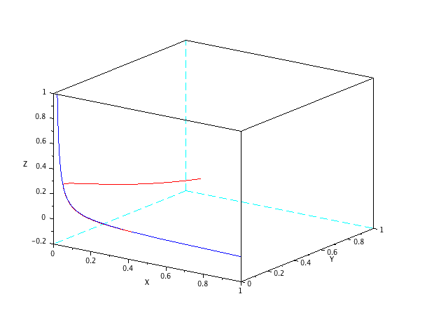
The results for the components are qualitatively similar to the fast vector dynamics, and hence are omitted. Nevertheless, the reduction of the dynamics to the slow manifold is more dramatic in this case as shown in figure 8.
Refer to caption
Figure 8. Slow manifold dynamics for the fast host regime. Parameter values are μ¯h=0.005subscript¯𝜇0.005\bar{\mu}_{h}=0.005, γ¯=0.4¯𝛾0.4\bar{\gamma}=0.4, δ¯=0.4¯𝛿0.4\bar{\delta}=0.4, μv=0.2subscript𝜇𝑣0.2\mu_{v}=0.2, and σ=0.5𝜎0.5\sigma=0.5.

6. Concluding remarks

As observed in the introduction, diseases that are vector-borne have a number of features that distinguish them from contagious ones. Typically, time scales for the dynamics of the host and vectors are not within the same order, since mosquitoes, for instance, that are a prevalent vector for such diseases have a very fast life cycle compared to humans. With this in mind, we investigated the dynamical consequences of having host and vector dynamics with distinct time scales in the classical arbovirus model introduced by [6, 18]. The natural regimes to look in this model are the fast vector dynamics (FVD) and fast host dynamics (FHD). While the former seems to be the most natural choice, we take the view that there might be scenarios where the latter may be observed.

By means of a formal multiscale asymptotic analysis, we study both regimes. For the FVD, we find the leading order dynamics yields a SIR model for the host, with a modified incidence rate. Thus, the vector is removed from the model being present only parametrically as a function of the host infected fraction. Such a relationship, apart from its mathematical interest, might also be useful in verifying if field data conforms, within the model, with the regime hypothesis. Additionally, the FHD regime yields an even more dramatic reduction with an SI model for the vectors, again with a modified incidence rate. Numerical results presented show that the approximation is indeed uniformly asymptotic in time. An interesting feature of the studied regimes is that they do not imply any condition on R0subscript𝑅0R_{0}, and hence are compatible with a variety of disease developments from the point of view of global dynamics. Indeed, for both reduced models, the equilibria are preserved by the asymptotic approximation, and the global stability dynamics is consistent with the global stability dynamics of the full model. Finally, we have confirmed rigorously the asymptotic character of the approximation up to the derived order. Due to the large variance of the parameters as measured in many different cases, we do not claim that these regimes are necessarily the most important, or the more prevalent. Nevertheless, they do provide a model problem where the reduction can be effectively carried out, and indicate how the dynamics can be described by such reduced models. In addition, the parameters that give rise to such regimes, particularly the Fast Vector Dynamics, are consistent with a number of concrete epidemiological scenarios.

The results obtained suggest that multiscaling reductions similar to the ones described here might be very effective in obtaining simplified models. In particular, as the complexity of models grows, we expect that such reductions may provide additional insights.

Appendix A Proof of Theorem 3

The proof of Theorem 3 is divided in several lemmas.

We write system (4) in a more concise form as

𝐖˙˙𝐖\displaystyle\dot{\mathbf{W}} =(𝐖,Z),absent𝐖𝑍\displaystyle=\mathcal{F}(\mathbf{W},Z),
ϵZ˙italic-ϵ˙𝑍\displaystyle\epsilon\dot{Z} =𝒢(𝐖,Z).absent𝒢𝐖𝑍\displaystyle=\mathcal{G}(\mathbf{W},Z).

with 𝐖(t)=(X(t),Y(t))t𝐖𝑡superscript𝑋𝑡𝑌𝑡𝑡\mathbf{W}(t)=(X(t),Y(t))^{t} and \mathcal{F} and 𝒢𝒢\mathcal{G} being the appropriate entries of the right hand side of (4). We write

𝐖=𝐖0+ϵ𝐖^0+ϵ𝐐andZ=Z0+Z^0+ϵZ¯,formulae-sequence𝐖superscript𝐖0italic-ϵsuperscript^𝐖0italic-ϵ𝐐and𝑍superscript𝑍0superscript^𝑍0italic-ϵ¯𝑍\mathbf{W}=\mathbf{W}^{0}+\epsilon\hat{\mathbf{W}}^{0}+\epsilon\mathbf{Q}\quad\text{and}\quad Z=Z^{0}+\hat{Z}^{0}+\epsilon\bar{Z},

with

𝐖^0=X0σ¯Y0+μ¯v(Z0σ¯Y0σ¯Y0+μ¯v)e(σ¯Y0+μ¯v)t/ϵ(1,1)t.superscript^𝐖0subscript𝑋0¯𝜎subscript𝑌0subscript¯𝜇𝑣subscript𝑍0¯𝜎subscript𝑌0¯𝜎subscript𝑌0subscript¯𝜇𝑣superscripte¯𝜎subscript𝑌0subscript¯𝜇𝑣𝑡italic-ϵsuperscript11𝑡\hat{\mathbf{W}}^{0}=\frac{X_{0}}{\bar{\sigma}Y_{0}+\bar{\mu}_{v}}\left(Z_{0}-\frac{\bar{\sigma}Y_{0}}{\bar{\sigma}Y_{0}+\bar{\mu}_{v}}\right)\mathrm{e}^{-(\bar{\sigma}Y_{0}+\bar{\mu}_{v})t/\epsilon}(1,-1)^{t}.

Notice that since 𝐖^0superscript^𝐖0\hat{\mathbf{W}}^{0} is bounded, we need only to prove that (𝐐,Z¯)𝐐¯𝑍(\mathbf{Q},\bar{Z}) exist, are bounded, and are unique. In this case, we then take C=(𝐐,Z¯)𝐶subscriptnorm𝐐¯𝑍C=\|(\mathbf{Q},\bar{Z})\|_{\infty}. First, we observe that

𝐖0˙+ϵ𝐖^0˙=(𝐖0,Z0+Z^0)+K(t)(1,1)tandZ^0˙=𝒢(𝐖0,Z0+Z^0)+L(t),formulae-sequence˙superscript𝐖0italic-ϵ˙superscript^𝐖0superscript𝐖0superscript𝑍0superscript^𝑍0𝐾𝑡superscript11𝑡and˙superscript^𝑍0𝒢superscript𝐖0superscript𝑍0superscript^𝑍0𝐿𝑡\dot{\mathbf{W}^{0}}+\epsilon\dot{\hat{\mathbf{W}}^{0}}=\mathcal{F}(\mathbf{W}^{0},Z^{0}+\hat{Z}^{0})+K(t)(1,-1)^{t}\quad\text{and}\quad\dot{\hat{Z}^{0}}=\mathcal{G}(\mathbf{W}^{0},Z^{0}+\hat{Z}^{0})+L(t),

where

K(t)=δZ^0(t/ϵ)(X0(t)X0)andL(t)=σ¯Z^0(t/ϵ)(Y0(t)Y0).formulae-sequence𝐾𝑡𝛿superscript^𝑍0𝑡italic-ϵsuperscript𝑋0𝑡subscript𝑋0and𝐿𝑡¯𝜎superscript^𝑍0𝑡italic-ϵsuperscript𝑌0𝑡subscript𝑌0K(t)=\delta\hat{Z}^{0}(t/\epsilon)(X^{0}(t)-X_{0})\quad\text{and}\quad L(t)=\bar{\sigma}\hat{Z}^{0}(t/\epsilon)(Y^{0}(t)-Y_{0}).

In particular, because of the fast decay of Z^0superscript^𝑍0\hat{Z}^{0}, and because L(0)=K(0)=0𝐿0𝐾00L(0)=K(0)=0, it follows that there exists a constant C>0𝐶0C>0, such that

0K(t)dt,0L(t)dtCϵ2.superscriptsubscript0𝐾𝑡differential-d𝑡superscriptsubscript0𝐿𝑡differential-d𝑡𝐶superscriptitalic-ϵ2\int_{0}^{\infty}K(t)\,\mathrm{d}t,\quad\int_{0}^{\infty}L(t)\,\mathrm{d}t\leq C\epsilon^{2}.

Since \mathcal{F} and 𝒢𝒢\mathcal{G} are quadratic, we write:

(𝐖,Z)=𝐖𝑍absent\displaystyle\mathcal{F}(\mathbf{W},Z)= (𝐖0,Z0+Z^0)+ϵD𝐖(𝐖0,Z0+Z^0)(𝐐+𝐖^0)+ϵDZ(𝐖0,Z0+Z^0)Z¯+superscript𝐖0superscript𝑍0superscript^𝑍0italic-ϵsubscript𝐷𝐖superscript𝐖0superscript𝑍0superscript^𝑍0𝐐superscript^𝐖0limit-fromitalic-ϵsubscript𝐷𝑍superscript𝐖0superscript𝑍0superscript^𝑍0¯𝑍\displaystyle\mathcal{F}(\mathbf{W}^{0},Z^{0}+\hat{Z}^{0})+\epsilon D_{\mathbf{W}}\mathcal{F}(\mathbf{W}^{0},Z^{0}+\hat{Z}^{0})(\mathbf{Q}+\hat{\mathbf{W}}^{0})+\epsilon D_{Z}\mathcal{F}(\mathbf{W}^{0},Z^{0}+\hat{Z}^{0})\bar{Z}+
+ϵ2δX¯Z¯(11);superscriptitalic-ϵ2𝛿¯𝑋¯𝑍matrix11\displaystyle\qquad+\epsilon^{2}\delta\bar{X}\bar{Z}\begin{pmatrix}-1\\ 1\end{pmatrix};
𝒢(𝐖,Z)=𝒢𝐖𝑍absent\displaystyle\mathcal{G}(\mathbf{W},Z)= 𝒢(𝐖0,Z0+Z^0)+ϵD𝐖𝒢(𝐖0,Z0+Z^0)(𝐐+𝐖^0)+ϵDZ𝒢(𝐖0,Z0+Z^0)Z¯+𝒢superscript𝐖0superscript𝑍0superscript^𝑍0italic-ϵsubscript𝐷𝐖𝒢superscript𝐖0superscript𝑍0superscript^𝑍0𝐐superscript^𝐖0limit-fromitalic-ϵsubscript𝐷𝑍𝒢superscript𝐖0superscript𝑍0superscript^𝑍0¯𝑍\displaystyle\mathcal{G}(\mathbf{W}^{0},Z^{0}+\hat{Z}^{0})+\epsilon D_{\mathbf{W}}\mathcal{G}(\mathbf{W}^{0},Z^{0}+\hat{Z}^{0})(\mathbf{Q}+\hat{\mathbf{W}}^{0})+\epsilon D_{Z}\mathcal{G}(\mathbf{W}^{0},Z^{0}+\hat{Z}^{0})\bar{Z}+
+ϵ2σ¯Y¯Z¯.superscriptitalic-ϵ2¯𝜎¯𝑌¯𝑍\displaystyle+\qquad\epsilon^{2}\bar{\sigma}\bar{Y}\bar{Z}.

where 𝐐=(X¯,Y¯)t𝐐superscript¯𝑋¯𝑌𝑡\mathbf{Q}=(\bar{X},\bar{Y})^{t}.

Let T(t,s)𝑇𝑡𝑠T(t,s) be the fundamental solution to the linearised system

(12) (𝐐˙ϵZ¯˙)=(D𝐖(𝐖0,Z0+Z^0)DZ(𝐖0,Z0+Z^0)D𝐖𝒢(𝐖0,Z0+Z^0)DZ𝒢(𝐖0,Z0+Z^0))(𝐐Z¯)matrix˙𝐐italic-ϵ˙¯𝑍matrixsubscript𝐷𝐖superscript𝐖0superscript𝑍0superscript^𝑍0subscript𝐷𝑍superscript𝐖0superscript𝑍0superscript^𝑍0subscript𝐷𝐖𝒢superscript𝐖0superscript𝑍0superscript^𝑍0subscript𝐷𝑍𝒢superscript𝐖0superscript𝑍0superscript^𝑍0matrix𝐐¯𝑍\begin{pmatrix}\dot{\mathbf{Q}}\\ \epsilon\dot{\bar{Z}}\end{pmatrix}=\begin{pmatrix}D_{\mathbf{W}}\mathcal{F}(\mathbf{W}^{0},Z^{0}+\hat{Z}^{0})&D_{Z}\mathcal{F}(\mathbf{W}^{0},Z^{0}+\hat{Z}^{0})\\ D_{\mathbf{W}}\mathcal{G}(\mathbf{W}^{0},Z^{0}+\hat{Z}^{0})&D_{Z}\mathcal{G}(\mathbf{W}^{0},Z^{0}+\hat{Z}^{0})\end{pmatrix}\begin{pmatrix}\mathbf{Q}\\ \bar{Z}\end{pmatrix}

Then direct integration yields

Lemma 1.

The functions (𝐐,Z¯)𝐐¯𝑍(\mathbf{Q},\bar{Z}) satisfy the following integral equation:

(𝐐Z¯)=matrix𝐐¯𝑍absent\displaystyle\begin{pmatrix}\mathbf{Q}\\ \bar{Z}\end{pmatrix}= T(t,0)(Q0Z¯0)+0tT(t,s)(ϵδX¯Z¯(11)σ¯Y¯Z¯)ds+𝑇𝑡0matrixsubscript𝑄0subscript¯𝑍0limit-fromsuperscriptsubscript0𝑡𝑇𝑡𝑠matrixitalic-ϵ𝛿¯𝑋¯𝑍matrix11¯𝜎¯𝑌¯𝑍differential-d𝑠\displaystyle T(t,0)\begin{pmatrix}Q_{0}\\ \bar{Z}_{0}\end{pmatrix}+\int_{0}^{t}T(t,s)\begin{pmatrix}\epsilon\delta\bar{X}\bar{Z}\begin{pmatrix}1\\ -1\end{pmatrix}\\ \bar{\sigma}\bar{Y}\bar{Z}\end{pmatrix}\,\mathrm{d}s+
(13) +0tT(t,s)(DW𝐖^0(s)DW𝒢𝐖^0(s)Z˙0(s))ds1ϵ20tT(t,s)(ϵK(s)(11)L(s))ds.superscriptsubscript0𝑡𝑇𝑡𝑠matrixsubscript𝐷𝑊superscript^𝐖0𝑠subscript𝐷𝑊𝒢superscript^𝐖0𝑠subscript˙𝑍0𝑠differential-d𝑠1superscriptitalic-ϵ2superscriptsubscript0𝑡𝑇𝑡𝑠matrixitalic-ϵ𝐾𝑠matrix11𝐿𝑠differential-d𝑠\displaystyle\qquad+\int_{0}^{t}T(t,s)\begin{pmatrix}D_{W}\mathcal{F}\cdot\hat{\mathbf{W}}^{0}(s)\\ D_{W}\mathcal{G}\cdot\hat{\mathbf{W}}^{0}(s)-\dot{Z}_{0}(s)\end{pmatrix}\,\mathrm{d}s-\frac{1}{\epsilon^{2}}\int_{0}^{t}T(t,s)\begin{pmatrix}\epsilon K(s)\begin{pmatrix}1\\ -1\end{pmatrix}\\ L(s)\end{pmatrix}\,\mathrm{d}s.

Moreover, the last term is bounded uniformly in ϵitalic-ϵ\epsilon.

We also have the following large time behaviour result for the linearised system (12):

Lemma 2.

Let (𝐐(t),Z¯(t))𝐐𝑡¯𝑍𝑡(\mathbf{Q}(t),\bar{Z}(t)) be a solution to (12). Then

limt(𝐐(t),Z¯(t))=𝟎.subscript𝑡𝐐𝑡¯𝑍𝑡0\lim_{t\to\infty}(\mathbf{Q}(t),\bar{Z}(t))=\mathbf{0}.

In particular, the solutions to (12) are bounded uniformly in time for any given ϵitalic-ϵ\epsilon. Moreover, they are also uniformly bounded in ϵ1italic-ϵ1\epsilon\leq 1, for all t0𝑡0t\geq 0.

Proof.

For notation convenience, let us write (12) as

(𝐐˙ϵZ¯˙)=A(𝐖0,Z0+Z^0)(𝐐Z¯).matrix˙𝐐italic-ϵ˙¯𝑍𝐴superscript𝐖0superscript𝑍0superscript^𝑍0matrix𝐐¯𝑍\begin{pmatrix}\dot{\mathbf{Q}}\\ \epsilon\dot{\bar{Z}}\end{pmatrix}=A(\mathbf{W}^{0},Z^{0}+\hat{Z}^{0})\begin{pmatrix}\mathbf{Q}\\ \bar{Z}\end{pmatrix}.

Fix ϵ>0italic-ϵ0\epsilon>0 and (X0,Y0,Z0)subscript𝑋0subscript𝑌0subscript𝑍0(X_{0},Y_{0},Z_{0}). From Theorem 2, we know that

limt(𝐖0(t),Z0(t)+Z^0(t/ϵ))=(𝐖,Z),subscript𝑡superscript𝐖0𝑡superscript𝑍0𝑡superscript^𝑍0𝑡italic-ϵsuperscript𝐖superscript𝑍\lim_{t\to\infty}\left(\mathbf{W}^{0}(t),Z^{0}(t)+\hat{Z}^{0}(t/\epsilon)\right)=(\mathbf{W}^{*},Z^{*}),

where (𝐖,Z)superscript𝐖superscript𝑍(\mathbf{W}^{*},Z^{*}) is the globally asymptotic stable equilibrium given by Theorem 1. Therefore, there exists T>0𝑇0T>0, such that t>T𝑡𝑇t>T implies that A𝐴A is negative-definite. Since Z^00superscript^𝑍00\hat{Z}^{0}\to 0, as ϵ0italic-ϵ0\epsilon\to 0. We can choose T𝑇T such this holds for all 0<ϵ10italic-ϵ10<\epsilon\leq 1.

Because of the continuity of the solution with respect to the initial conditions, we have that T𝑇T is a continuous function of the initial conditions. Since these lie on a compact set, we can pick T𝑇T such that A𝐴A is negative definite for all 0<ϵ10italic-ϵ10<\epsilon\leq 1 and for all (X0,Y0,Z0)subscript𝑋0subscript𝑌0subscript𝑍0(X_{0},Y_{0},Z_{0}), such that X0,Y00subscript𝑋0subscript𝑌00X_{0},Y_{0}\geq 0, X0+Y01subscript𝑋0subscript𝑌01X_{0}+Y_{0}\leq 1 and 0<Z010subscript𝑍010<Z_{0}\leq 1. But then, for any such (X0,Y0,Z0)subscript𝑋0subscript𝑌0subscript𝑍0(X_{0},Y_{0},Z_{0}) and 0<ϵ10italic-ϵ10<\epsilon\leq 1, we have that

limtT(t,T)=0.subscript𝑡𝑇𝑡𝑇0\lim_{t\to\infty}T(t,T)=0.

Therefore, for any initial condition (Q0,Z¯0)tsuperscriptsubscript𝑄0subscript¯𝑍0𝑡(Q_{0},\bar{Z}_{0})^{t}, we have

limtT(t,0)(Q0Z¯0)=limtT(t,T)T(T,0)(Q0Z¯0)=0.subscript𝑡𝑇𝑡0matrixsubscript𝑄0subscript¯𝑍0subscript𝑡𝑇𝑡𝑇𝑇𝑇0matrixsubscript𝑄0subscript¯𝑍00\lim_{t\to\infty}T(t,0)\begin{pmatrix}Q_{0}\\ \bar{Z}_{0}\end{pmatrix}=\lim_{t\to\infty}T(t,T)T(T,0)\begin{pmatrix}Q_{0}\\ \bar{Z}_{0}\end{pmatrix}=0.

square-intersection\sqcapsquare-union\sqcup

square-intersection\sqcapsquare-union\sqcup

Proof of Theorem 3.

First, we observe that the nonlinear term in (13) is locally Lipschitz, hence a standard fixed point yields existence and uniqueness for 0t<t00𝑡subscript𝑡00\leq t<t_{0} , for some, possibly small, t0subscript𝑡0t_{0}.

From the decaying of 𝐖^0superscript^𝐖0\hat{\mathbf{W}}^{0} and from Lemma 1, we conclude that the two last terms of (13) are uniformly bounded in time and ϵitalic-ϵ\epsilon.

Moreover, Lemma 2 implies that the first two terms on the right hand side of (13) are also uniformly bounded in time and in ϵitalic-ϵ\epsilon, for sufficiently small ϵitalic-ϵ\epsilon. Thus, we conclude that the same also holds true for (Q,R)tsuperscript𝑄𝑅𝑡(Q,R)^{t}. Therefore, the solution to (13) is globally defined in time, and it is bounded uniformly in ϵitalic-ϵ\epsilon, if the latter is sufficiently small.

square-intersection\sqcapsquare-union\sqcup

square-intersection\sqcapsquare-union\sqcup

References

  • [1] B. Adams and M. Boots. How important is vertical transmission in mosquitoes for the persistence of dengue? insights from a mathematical model. Epidemics, 2(1):1–10, Mar 2010.
  • [2] M. Aguiar, S. Ballesteros, B. W. Kooi, and N. Stollenwerk. The role of seasonality and import in a minimalistic multi-strain dengue model capturing differences between primary and secondary infections: complex dynamics and its implications for data analysis. J Theor Biol, 289:181–96, Nov 2011.
  • [3] A. Aldemir, H. Bedir, B. Demirci, and B. Alten. Biting activity of mosquito species (diptera: Culicidae) in the turkey-armenia border area, ararat valley, turkey. J Med Entomol, 47(1):22–7, Jan 2010.
  • [4] R. M. Anderson and R. M. May. Infectious diseases of humans: dynamics and control. Oxford science publications. Oxford University Press, Oxford ¡etc.¿, ¡1st ed. 1991, repr.¿ edition, 1995.
  • [5] M. Andraud, N. Hens, C. Marais, and P. Beutels. Dynamic epidemiological models for dengue transmission: a systematic review of structural approaches. PLoS One, 7(11):e49085, 2012.
  • [6] N. T. J. Bailey. The mathematical theory of infectious diseases. Griffin, 1975.
  • [7] R. Barrera, M. Amador, and G. G. Clark. Ecological factors influencing aedes aegypti (diptera: Culicidae) productivity in artificial containers in salinas, puerto rico. Journal of Medical Entomology, 43(3):484–492, 2006.
  • [8] J. G. Breman. Resistance to artemisinin-based combination therapy. The Lancet Infectious Diseases, 12(11):820–822, 11 2012.
  • [9] N. Britton. Essential mathematical biology. Springer Verlag, 2003.
  • [10] L. Cai, S. Guo, X. Li, and M. Ghosh. Global dynamics of a dengue epidemic mathematical model. Chaos, Solitons & Fractals, 42(4):2297–2304, Nov. 2009.
  • [11] CDC. Geographic distribution of chikungunya virus.
  • [12] C. Chastel. Eventual role of asymptomatic cases of dengue for the introduction and spread of dengue viruses in non-endemic regions. Front Physiol, 3:70, 2012.
  • [13] S.-C. Chen and M.-H. Hsieh. Modeling the transmission dynamics of dengue fever: implications of temperature effects. Sci Total Environ, 431:385–91, Aug 2012.
  • [14] F. Dantas-Torres, B. B. Chomel, and D. Otranto. Ticks and tick-borne diseases: a one health perspective. Trends Parasitol, 28(10):437–46, Oct 2012.
  • [15] M. R. David, R. L. de Oliveira, and R. M. de Freitas. Container productivity, daily survival rates and dispersal of aedes aegypti mosquitoes in a high income dengue epidemic neighbourhood of rio de janeiro: presumed influence of differential urban structure on mosquito biology. Mem Inst Oswaldo Cruz, 104:927–932,, 2009.
  • [16] J.-C. Desenclos. Transmission parameters of vector-borne infections. Med Mal Infect, 41(11):588–93, Nov 2011.
  • [17] O. Diekmann and J. Heesterbeek. Mathematical epidemiology of infectious diseases: model building, analysis and interpretation. Wiley series in mathematical and computational biology. Wiley, Chichester, 2000.
  • [18] K. Dietz. Transmission and control of arbovirus diseases. In D. Ludwig and K. L. Cooke, editors, Epidemiology, pages 104–121. SIAM, 1975.
  • [19] L. Esteva and C. Vargas. Analysis of a dengue disease transmission model. Mathematical Biosciences, 150(2):131–151, June 1998.
  • [20] M. G. The epidemiology and control of malaria. Oxford: Oxford University Press, 1957.
  • [21] N. C. Grassly and C. Fraser. Mathematical models of infectious disease transmission. Nat Rev Micro, 6(6):477–487, 06 2008.
  • [22] N. G. Gratz. Critical review of the vector status of aedes albopictus. Medical and Veterinary Entomology, 18(3):215–227, 2004.
  • [23] D. J. Gubler. Dengue and dengue hemorrhagic fever. Clin Microbiol Rev, 11(3):480–96, Jul 1998.
  • [24] K. JC. On the use of mathematical models of malaria transmission. Acta Trop, 49(1):1–25, 1991.
  • [25] L. Lambrechts, T. W. Scott, and D. J. Gubler. Consequences of the expanding global distribution of aedes albopictus for dengue virus transmission. PLoS Negl Trop Dis, 4(5):e646, 2010.
  • [26] C. C. Lord. Modeling and biological control of mosquitoes. J Am Mosq Control Assoc, 23(2 Suppl):252–64, 2007.
  • [27] P. M. Luz, C. T. Codeço, E. Massad, and C. J. Struchiner. Uncertainties regarding dengue modeling in rio de janeiro, brazil. Mem Inst Oswaldo Cruz, 98(7):871–8, Oct 2003.
  • [28] P. M. Luz, C. T. Codeço, J. Medlock, C. J. Struchiner, D. Valle, and A. P. Galvani. Impact of insecticide interventions on the abundance and resistance profile of aedes aegypti. Epidemiol Infect, 137(8):1203–15, Aug 2009.
  • [29] P. M. Luz, C. J. Struchiner, and A. P. Galvani. Modeling transmission dynamics and control of vector-borne neglected tropical diseases. PLoS Negl Trop Dis, 4(10):e761, 2010.
  • [30] S. Mandal, R. R. Sarkar, and S. Sinha. Mathematical models of malaria–a review. Malar J, 10:202, 2011.
  • [31] L. E. Muir and B. H. Kay. Aedes aegypti survival and dispersal estimated by mark-release-recapture in northern australia. Am J Trop Med Hyg, 58(3):277–82, Mar 1998.
  • [32] J. D. Murray. Mathematical biology, volume Vol. 17-18 of Interdisciplinary applied mathematics. Springer, New York, 3rd ed edition, 2002.
  • [33] G. Ngwa and W. Shu. A mathematical model for endemic malaria with variable human and mosquito populations. Math. Comput. Model., 32(7-8):747–763, Oct. 2000.
  • [34] H. Nishiura. Mathematical and statistical analyses of the spread of dengue. Dengue Bulletin, 30:51–67, 2006.
  • [35] L. C. Okell, C. J. Drakeley, T. Bousema, C. J. M. Whitty, and A. C. Ghani. Modelling the impact of artemisinin combination therapy and long-acting treatments on malaria transmission intensity. PLoS Med, 5(11):e226; discussion e226, Nov 2008.
  • [36] R. O’Malley. Singular perturbation methods for ordinary differential equations. Springer, 1991.
  • [37] L. R. Petersen and M. Fischer. Unpredictable and difficult to control–the adolescence of west nile virus. N Engl J Med, 367(14):1281–4, Oct 2012.
  • [38] A. M. Powers. Chikungunya. Clin Lab Med, 30(1):209–19, Mar 2010.
  • [39] A. M. Powers, A. C. Brault, R. B. Tesh, and S. C. Weaver. Re-emergence of chikungunya and o’nyong-nyong viruses: evidence for distinct geographical lineages and distant evolutionary relationships. J Gen Virol, 81(Pt 2):471–9, Feb 2000.
  • [40] R. R. The prevention of malaria. London: Murray, 2nd edition, 1911.
  • [41] S. Rajapakse, C. Rodrigo, and A. Rajapakse. Atypical manifestations of chikungunya infection. Trans R Soc Trop Med Hyg, 104(2):89–96, Feb 2010.
  • [42] T. W. Scott, P. H. Amerasinghe, A. C. Morrison, L. H. Lorenz, G. G. Clark, D. Strickman, P. Kittayapong, and J. D. Edman. Longitudinal studies of aedes aegypti (diptera: Culicidae) in thailand and puerto rico: blood feeding frequency. J Med Entomol, 37(1):89–101, Jan 2000.
  • [43] T. W. Scott, E. Chow, D. Strickman, P. Kittayapong, R. A. Wirtz, L. H. Lorenz, and J. D. Edman. Blood-feeding patterns of aedes aegypti (diptera: Culicidae) collected in a rural thai village. J Med Entomol, 30(5):922–7, Sep 1993.
  • [44] T. W. Scott, A. C. Morrison, L. H. Lorenz, G. G. Clark, D. Strickman, P. Kittayapong, H. Zhou, and J. D. Edman. Longitudinal studies of aedes aegypti (diptera: Culicidae) in thailand and puerto rico: population dynamics. J Med Entomol, 37(1):77–88, Jan 2000.
  • [45] D. L. Smith, K. E. Battle, S. I. Hay, C. M. Barker, T. W. Scott, and F. E. McKenzie. Ross, Macdonald, and a theory for the dynamics and control of mosquito-transmitted pathogens. PLoS Pathog, 8(4):e1002588, 2012.
  • [46] L. M. Styer, S. L. Minnick, A. K. Sun, and T. W. Scott. Mortality and reproductive dynamics of aedes aegypti (diptera: Culicidae) fed human blood. Vector Borne Zoonotic Dis, 7(1):86–98, 2007.
  • [47] J. J. Tewa, J. L. Dimi, and S. Bowong. Lyapunov functions for a dengue disease transmission model. Chaos, Solitons & Fractals, 39(2):936–941, Jan. 2009.
  • [48] O. Tomori. Yellow fever: the recurring plague. Crit Rev Clin Lab Sci, 41(4):391–427, 2004.
  • [49] WHO. Dengue and severe dengue.
  • [50] H. Yang, H. Wei, and X. Li. Global stability of an epidemic model for vector-borne disease, 2010-04-01.
  • [51] H. M. Yang, M. L. G. Macoris, K. C. Galvani, M. T. M. Andrighetti, and D. M. V. Wanderley. Assessing the effects of temperature on dengue transmission. Epidemiol Infect, 137(8):1179–87, Aug 2009.
  • [52] H. M. Yang, M. L. G. Macoris, K. C. Galvani, M. T. M. Andrighetti, and D. M. V. Wanderley. Assessing the effects of temperature on the population of aedes aegypti, the vector of dengue. Epidemiol Infect, 137(8):1188–202, Aug 2009.