Instability of Ginzburg-Landau Vortices on Manifolds

Abstract

We investigate two settings of Ginzburg-Landau posed on a manifold where vortices are unstable. The first is an instability result for critical points with vortices of the Ginzburg-Landau energy posed on a simply connected, compact, closed $2$-manifold. The second is a vortex annihilation result for the Ginzburg-Landau heat flow posed on certain surfaces of revolution with boundary.

1 Introduction

In this paper we consider the Ginzburg-Landau energy posed on a $2$-manifold. We will present two results, one for critical points of the Ginzburg-Landau energy and one for the Ginzburg-Landau heat flow, both showing the non-existence of stable vortex solutions under certain geometric assumptions on the manifold. We say a critical point is unstable if there is a direction in which the second variation of the energy is negative. For the heat flow, we will show that all initial data, even those containing vortices, will eventually converge to a vortex-free solution.

Let $E_{\varepsilon}$ be Ginzburg-Landau energy on an orientable manifold $\cal M$ equipped with a metric $g$ for $u:\cal M\rightarrow\mathbb{C}$,

$$E_{\varepsilon}(u)=\frac{1}{2}\int_{\cal M}||\nabla_{g}u||_{g}^{2}+\frac{(1-|u|^{2})^{2}}{2\varepsilon^{2}}dv_{g}.$$

There is a vast literature on Ginzburg-Landau, but we review here just a few of the results most closely related to our investigation. When $\cal M$ is a bounded domain $\Omega\subset\mathbb{R}^{2}$, and under an $S^{1}$-valued Dirichlet condition, Bethuel, Brezis and Hélein establish in [4] that vortices of minimizers converge as $\varepsilon\rightarrow 0$ to a finite set of points or limiting vortices $\{a_{i}\}$. Here vortices refer to zeros of the order parameter $u_{\varepsilon}$ carrying nonzero degree. Moreover, the limiting vortex locations $\{a_{i}\}$ will minimize a renormalized energy $W$. Another important result comes in [7] where for $u:{\cal M}=\Omega\subset\mathbb{R}^{n}\rightarrow\mathbb{R}^{N}$, Jimbo and Morita prove that under homogeneous Neumann boundary conditions, if $\Omega$ is convex, the only stable critical points are constants for any $\varepsilon>0$.

Most important to our work on stability of critical points is the work of Serfaty in [10] on Ginzburg-Landau in simply connected planar domains. Here she shows that there is no nonconstant stable critical point of $E_{\varepsilon}$ with homogeneous Neumann boundary conditions for $\varepsilon$ small. To achieve this, she shows that the renormalized energy has no stable critical points. Then using her theory of “$C^{2}$-Gamma convergence,” she argues that there must be unstable directions for the Hessian of $E_{\varepsilon}$ as well for $\varepsilon$ small. Our first main result (Theorem 2.1) in this paper is that for compact, simply connected $2$-manifolds without boundary, any critical points must be unstable when $\varepsilon$ is small if at least one limiting vortex is located at a point of positive Gauss curvature. Furthermore, if one additionally assumes that ${\cal M}$ is a surface of revolution with non-zero Gauss curvature at at least one of the poles, then we argue that all critical points are unstable for $\varepsilon$ small, regardless of the curvature of the manifold at the limiting vortex locations (Theorem 2.3). To prove this, we will apply Serfaty’s abstract result in [10] (see Theorem 2.2 below), showing again that the renormalized energy has no stable critical points on such manifolds. For Ginzburg-Landau posed on a $2$-manifold, Baraket generalizes the work of [4] to identify the renormalized energy on compact $2$-manifolds without boundary in [1]. We should perhaps note that for Ginzburg-Landau in $3$-dimensional domains, there do exist stable vortex solutions ([9]). This analysis will be presented in Section 2.

The second setting we consider is the heat flow for the Ginzburg-Landau energy, with $\varepsilon=1$, on surfaces of revolution ${\cal M}$ with boundary:

$$\left\{\begin{array}[]{ll}u_{t}-\bigtriangleup_{\cal M}u=(1-|u|^{2})u&\mbox{in $\cal M\times\mathbb{R}_{+}$},\\ u=e&\mbox{on $\partial\cal M\times\mathbb{R}_{+}$},\\ u=u_{0}&\mbox{on $\cal M\times$$\{t=0\}.$}\end{array}\right.$$

Here $u:\cal M\times\mathbb{R}_{+}\rightarrow\mathbb{R}$², and $e$ is any constant unit vector. We allow the compatible initial data $u_{0}$ to have any number of vortices though necessarily the total degree $\sum d_{i}=0$ in light of the Dirichlet condition. We want to find conditions on $\cal M$ such that as $t\rightarrow\infty$, all vortices are annihilated. When ${\cal M}=\mathbb{R}^{2}$, it has been shown in [2] that if $u_{0}$ is close to $e$ at infinity in some sense, all vortices of $u$ disappear after a finite time. As in [2], we will derive a Pohozaev-type inequality on surfaces (Lemma 3.3) to prove a similar result when $\cal M$ is a simply connected surface of revolution satisfying an extra geometric assumption that is unrelated to curvature, see Theorem 3.1. This work is presented in Section 3.

2 Instability of Critical Points on a Compact Surface

In this section we take $\cal M$ to be a simply connected compact surface without boundary, and $g$ be a metric on $\cal M$. Consider the Ginzburg-Landay energy on $\cal M$,

$$E_{\varepsilon}(u)=\frac{1}{2}\int_{\cal M}||\nabla_{g}u||_{g}^{2}+\frac{(1-|u|^{2})^{2}}{2\varepsilon^{2}}dv_{g}$$ (2.1)

where $u\in H^{1}(\cal M,\mathbb{C})$. Let $u_{\varepsilon}$ be the critical point of (2.1), then $u_{\varepsilon}$ satisfies

$$-\bigtriangleup_{g}u_{\varepsilon}=\frac{u_{\epsilon}(1-|u_{\epsilon}|^{2})}{\varepsilon^{2}}\mbox{ in }\cal M$$ (2.2)

In [4] where $\cal M$ is a bounded planer domain, Bethuel, Brezis and Hélein prove that under an $S^{1}$-valued Dirichlet boundary condition, critical points $u_{\varepsilon}$ of (2.1) converges to a limiting map $u_{*}$ strongly in $C^{k}_{loc}({\cal M}\setminus\bigcup_{i=1}^{n}a_{i})$ for every integer $k$ and in $C^{1,\alpha}_{loc}(\bar{\cal M}\setminus\bigcup_{i=1}^{n}a_{i})$ for $\alpha<1$ where $\{a_{i}\}$ is a finite set. This result has been generalized to a compact manifold $\cal M$ without boundary, cf. [1, 6] and has since been refined, see e.g. [8] and [12]. Thus, we have:

Proposition 2.1.

Let $\{u_{\varepsilon}\}$ be a sequence of critical points of $E_{\varepsilon}$ with $E_{\varepsilon}(u_{\epsilon})\leq C|\log\varepsilon|$ for some constant $C>0$. Then up to extraction of a subsequence, there exists a finite set of points $a_{1},...,a_{n}$ in $\cal M$ such that $u_{\varepsilon}\rightarrow u_{*}$ strongly in $W^{1,p}(\cal M)$ for $p<2$ and in $H^{1}_{loc}$$(\cal M$$\setminus\bigcup_{i=1}^{n}a_{i})$.

We will refer to these points $a_{1},...,a_{n}$ as limiting vortices associates with the sequence $\{u_{\varepsilon}\}$.The same result holds on a compact manifold with modifications, see Proposition 5.5 in [6].

From the Uniformization Theorem, there is a conformal map $h:\cal M\rightarrow\mathbb{R}$${}^{2}\bigcup\{\infty\}$, so that the metric $g$ is given by $e^{2f}(dx_{1}^{2}+dx_{2}^{2})$ for some smooth function $f$. We recall that $\bigtriangleup f=-K_{\cal M}e^{2f}$, where $K_{\cal M}$ is the Gauss curvature on $\cal M$. Then for $U_{\varepsilon}:=u_{\varepsilon}\circ h^{-1}$, (2.2) transforms to

$$-\bigtriangleup U_{\varepsilon}=\frac{e^{2f}}{\varepsilon^{2}}U_{\varepsilon}(1-|U_{\varepsilon}|^{2})\mbox{ in }\mathbb{R}^{2}.$$ (2.3)

We may assume that $h(a_{i})\neq\infty$ for all $i$ and denote $b_{i}:=h(a_{i})$. With a slight abuse of terminology, we will also call the $b_{i}$’s limiting vortices. Then $u_{*}$ is the harmonic map associated to $(b_{i},d_{i})$:

$$u_{*}(x)=\prod_{i=1}^{n}(\frac{x-b_{i}}{|x-b_{i}|})^{d_{i}}e^{i\psi}\mbox{ in }\mathbb{R}^{2},$$ (2.4)

where $d_{i}\in\mathbb{Z}\setminus\{0\}$, $\sum_{i=1}^{n}d_{i}=0$, and $\psi$ is a smooth harmonic function. We also note that the notion of convergence linking $\{u_{\varepsilon}\}$ to $\{a_{i}\}$ is that of convergence of the sequence of Jacobians, namely

$$curl(iU_{\varepsilon},\nabla U_{\varepsilon})\rightharpoonup 2\pi\sum_{i=1}^{n}d_{i}\delta_{b_{i}}$$

in the sense of distributions, where $(\cdot,\cdot)$ denotes the scalar product in $\mathbb{C}$. For Euclidean domains, the proof of this convergence of Jacobians can be found in [8, 12] and the adaptation to the manifold setting is immediate. Moreover, the renormalized energy can be defined in the following way:

Given $\{a_{i}\}_{i=1}^{n}\subset\cal M$, let $B_{i}^{g}(r)$ be the geodesic ball in $\cal M$ centered at $a_{i}$ with radius $r$, and $B_{i}(r)=h(B_{i}^{g}(r))\subset\mathbb{R}^{2}$. Consider $\Phi_{r}$ which satisfies

$$\left\{\begin{array}[]{ll}\bigtriangleup\Phi_{r}=0&\mbox{in }\mathbb{R}^{2}\setminus\bigcup_{i=1}^{n}B_{i}(r)\\ \Phi_{r}=const.&\mbox{on each }\partial B_{i}(r)\\ \int_{\partial B_{i}(r)}\frac{\partial\Phi_{r}}{\partial\nu}=2\pi d_{i}&\mbox{for }1\leq i\leq n.\end{array}\right.$$ (2.5)

To see the existence of such a solution $\Phi_{r}$, we first consider a functional

$$E(v)=\int_{\cal M}|\nabla_{g}v|^{2}-2\pi\sum_{i=1}^{n}d_{i}v|_{\partial B_{i}^{g}(r)}$$

defined for $v\in H^{1}(\cal M)$ such that $v|_{\partial B_{i}^{g}(r)}=const.$ for each $i$. Using the direct method one can show that there exists a minimizer $v_{*}$ of $E$. Then since $g$ is a conformal metric, $v_{*}\circ h^{-1}$ satisfies (2.5). The renormalized energy is defined by

$$W(\mathbf{b})=\lim_{r\rightarrow 0}\frac{1}{2}\int_{\mathbb{R}^{2}\setminus\bigcup_{i=1}^{n}B_{i}(r)}|\nabla\Phi_{r}|^{2}dx-\pi\sum_{i=1}^{n}d_{i}^{2}\log\frac{1}{r},$$ (2.6)

where $\mathbf{b}=(b_{1},...,b_{n})$.

Finally, using the fact that $\Phi_{r}(x)\approx\sum_{i=1}^{n}d_{i}\log|x-b_{i}|$ for $x\in\mathbb{R}^{2}\setminus\bigcup_{i=1}^{n}B_{i}(r)$ when $r\ll 1$, Theorem 2.1 in [1] establishes that $W$ can be written as

$$W(\mathbf{b})=\pi\sum_{i=1}^{n}d_{i}^{2}f(b_{i})-\pi\sum_{i\neq j}d_{i}d_{j}\log|b_{i}-b_{j}|.$$ (2.7)

Our first main result is the following:

Theorem 2.1.

Let $\{u_{\varepsilon}\}$ be a family of solutions to (2.3) such that $E_{\varepsilon}(u_{\varepsilon})\leq C|\log\varepsilon|$, and let $\{a_{i}\}_{i=1}^{n}\subset\cal M$ be the limiting vortices for $\{u_{\varepsilon}\}$. Suppose there exists an $a_{i}$ such that the Gauss curvature $K_{\cal M}$ is positive at $a_{i}$. Then for $\varepsilon$ small enough, $u_{\varepsilon}$ is unstable.

Remark 2.1.

Theorem 2.1 implies that if $\cal M$ has positive curvature everywhere, then there is no stable solution to (2.3) having vortices for $\varepsilon$ small enough. Moreover, in this case any solution without any vortices must then be a constant (see Lemma 3.2 in the next section). For the special case where $\cal M=S^{2}$, this instability result was first obtained by Contreras, [5]

Remark 2.2 (The Apple Problem).

If one wants to look for an example of a stable nonconstant critical point, one might consider a surface of revolution $\cal A$ obtained by rotating a smooth curve $\Gamma$ about the $z$-axis shown in Figure 1, so that the shape of $\cal A$ is like an apple. Indeed, one can easily construct a critical point with vortices at $S$ and $N$ (cf. [6]), but it cannot be stable in view of Theorem 2.1, since $K_{\cal A}$ is positive at poles $N$ and $S$. We note that for the 3-D case (solid apple in $\mathbb{R}^{3}$), it has been proven in [9] that a critical point with a vortex line through $S$ and $N$ is a local minimizer for $\varepsilon$ small enough.

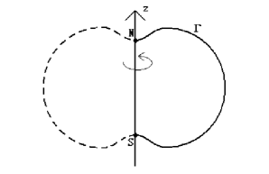
Figure 1: Surface of revolution $\cal A$

To prove Theorem 2.1, our main tool will be Serfaty’s abstract result in [10] for any $C^{2}$ functionals $F_{\varepsilon}$ (resp. $F$) defined over $\cal S$ (resp. $\cal S^{\prime}$), which is an open set of an affine space associated to a Banach space $\cal B$ (resp. $\cal B^{\prime}$) satisfying a kind of “$C^{2}$ $\Gamma$-convergence”. Let $u_{\varepsilon}\in\cal S$ be a family of critical points of $F_{\varepsilon}$. Assume $u_{\varepsilon}$ converges to $u\in S^{\prime}$ in some topology. Then denoting by $n_{\varepsilon}^{-}$ (resp. $n^{-}$) the dimension of the space spanned by eigenvectors of $D^{2}F_{\varepsilon}(u_{\varepsilon})$ defined over $\cal B$ (resp. $D^{2}F(u)$ defined over $\cal B^{\prime}$) associated to negative eigenvalues, the theorem states

Theorem 2.2 ([10]).

Suppose that for any $V\in\cal B^{\prime}$, there exists $v_{\varepsilon}(t)\in\cal S$ defined in a neighborhood of $t=0$ such that

$$v_{\varepsilon}(0)=u_{\varepsilon},$$ (2.8)

$$\partial_{t}v_{\varepsilon}(0)\mbox{ is a one-to-one linear map on }\cal B^{\prime},$$ (2.9)

$$\lim_{\varepsilon\rightarrow 0}\frac{d}{dt}|_{t=0}F_{\varepsilon}(v_{\varepsilon}(t))=\frac{d}{dt}|_{t=0}F(u+tV),$$ (2.10)

$$\lim_{\varepsilon\rightarrow 0}\frac{d^{2}}{dt^{2}}|_{t=0}F_{\varepsilon}(v_{\varepsilon}(t))=\frac{d^{2}}{dt^{2}}|_{t=0}F(u+tV).$$ (2.11)

Then for $\varepsilon$ small enough, we have $n_{\varepsilon}^{-}\geq n^{-}$.

In the same paper, she applies this result to Ginzburg-Landau in bounded domains in $\mathbb{R}^{2}$ with homogeneous Neumann boundary conditions. In a similar manner, to prove Theorem 2.1, we apply this approach to Ginzburg-Landau on surfaces. That is, using the same notation as above we shall prove

Proposition 2.2.

Let $u_{\varepsilon}$ be a family of critical points of $E_{\varepsilon}$ such that $E_{\varepsilon}(u_{\varepsilon})\leq C|\log\varepsilon|$, and $b_{1},b_{2},...,b_{n}$ be limiting vortices with total degree zero. Then hypotheses (2.8) to (2.11) in Theorem 2.2 hold for $F_{\varepsilon}=E_{\varepsilon}$, $F=W$ and $\cal B^{\prime}=$$\mathbb{V}$$=\{(V_{1},V_{2},...,V_{n}):V_{i}\in{\mathbb{R}^{2}}\;\forall 1\leq i\leq n\}$.

Proof.

Let $u_{\varepsilon}$ be a family of critical points of $E_{\varepsilon}$ such that $E_{\varepsilon}(u_{\varepsilon})\leq C|\log\varepsilon|$. Then from results in [1] (see also [6]), there exists $\rho>0$ small enough such that $B_{i}^{g}(\rho)$ are disjoint with $|u_{\varepsilon}|\geq\frac{1}{2}$ in $\cal M\setminus$$\bigcup_{i=1}^{n}$ $B_{i}^{g}(\rho)$ for $\varepsilon$ small enough.

The construction of $v_{\varepsilon}(t)$ is based on Propsition III.1 in [10]. Let $B_{i}=B_{i}(\rho)=h(B_{i}^{g}(\rho))$. For a given $\mathbf{V}\in\mathbb{V}$, we can define a $C^{1}$ family of diffeomorphisms of $\mathbb{R}^{2}$, $\chi_{t}(x)=x+t\mathbf{X}(x)$, in a neighborhood of $t=0$ such that $\mathbf{X}$ has compact support in a set $K\subset\subset\mathbb{R}^{2}$ and

$$\mathbf{X}(x)=V_{i}\mbox{ in each }B_{i}.$$

Then we define $\Phi_{0,t}$ by

$$\bigtriangleup\Phi_{0,t}=2\pi\sum_{i=1}^{n}d_{i}\delta_{b_{i}(t)}\mbox{ in }\mathbb{R}^{2},$$ (2.12)

so that $\Phi_{0,t}(x)=\sum_{i=1}^{n}d_{i}\log|x-b_{i}(t)|$, and let $\Phi_{0,0}=\Phi_{0}$, where $b_{i}(t)=\chi_{t}(b_{i})$. Then we denote by $\theta_{t}^{i}$ the polar coordinate centered at $b_{i}(t)$, and let

$$\psi_{t}=\sum_{i=1}^{n}d_{i}\theta_{t}^{i}\circ\chi_{t}-\sum_{i=1}^{n}d_{i}\theta_{0}^{i}.$$

Then we have

$$\nabla^{\perp}\Phi_{0}+\nabla\psi_{t}=\nabla(\sum_{i=1}^{n}d_{i}\theta_{t}^{j}\circ\chi_{t}).$$ (2.13)

Finally we define $v_{\varepsilon}(\chi_{t}(x),t)=u_{\varepsilon}(x)e^{i\psi_{t}(x)}$. With the same argument as in [10], one can show that (2.8) and (2.9) hold for $v_{\varepsilon}$. Since $\mathbf{X}$ is compactly supported, the domain of integration reduces from $\mathbb{R}^{2}$ to a compact set. Consequently, the result of product-estimate derived in [11] used in the original proof can be also applied in our case. Therefore we proceed to verify (2.10).

By the change of variables $y=\chi_{t}(x)$, we have

$$E_{\varepsilon}(v_{\varepsilon}) =\frac{1}{2}\int_{\mathbb{R}^{2}}|\nabla v_{\varepsilon}(y)|^{2}+\frac{e^{2f(y)}}{2\varepsilon^{2}}(1-|v_{\varepsilon}|^{2})^{2}dy$$

$$=\frac{1}{2}\int_{\mathbb{R}^{2}}|\nabla(u_{\varepsilon}e^{i\psi_{t}})(D\chi_{t})^{-1}|^{2}+\frac{e^{2f(\chi_{t})}}{2\varepsilon^{2}}(1-|u_{\varepsilon}|^{2})^{2}|Jac\;\chi_{t}|dx.$$ (2.14)

Noting that $\chi_{t}$ is the identity map in $\mathbb{R}^{2}\setminus K$ and a translation along a constant vector $V_{i}$ in each $B_{i}$, we deduce that in $\mathbb{R}^{2}\setminus K$ and $\bigcup_{i=1}^{n}B_{i}$,

$$\frac{d}{dt}(D\chi_{t})^{-1}=\frac{d^{2}}{dt^{2}}(D\chi_{t})^{-1}=\frac{d}{dt}|Jac\;\chi_{t}|=\frac{d^{2}}{dt^{2}}|Jac\;\chi_{t}|=0.$$ (2.15)

-Derivative of the potential term:

From (2.15), we derive

$$\frac{d}{dt}|_{t=0} \int_{\mathbb{R}^{2}}\frac{e^{2f(\chi_{t})}}{4\varepsilon^{2}}(1-|u_{\varepsilon}^{2}|)^{2}|Jac\;\chi_{t}|dx$$

$$= \int_{K\setminus\bigcup_{i=1}^{n}B_{i}}\frac{e^{2f(\chi_{t})}}{2\varepsilon^{2}}(1-|u_{\varepsilon}^{2}|)^{2}\;\nabla f\cdot\mathbf{X}dx$$

$$+\int_{K\setminus\bigcup_{i=1}^{n}B_{i}}\frac{e^{2f(\chi_{t})}}{2\varepsilon^{2}}(1-|u_{\varepsilon}^{2}|)^{2}\frac{d}{dt}|_{t=0}|Jac\;\chi_{t}|dx$$ (2.16)

Since $\nabla f\cdot\mathbf{X}$ and $\frac{d}{dt}|_{t=0}|Jac\;\chi_{t}|$ are bounded in $K\setminus\bigcup_{i=1}^{n}B_{i}$, one can apply Lemma 3.2 in [1] which asserts that $\frac{e^{2f}}{\varepsilon}(1-|u_{\varepsilon}|^{2})^{2}$ converges to a measure supported on $\bigcup_{i=1}^{n}b_{i}$. Hence, we have

$$\frac{d}{dt}|_{t=0}\int_{\mathbb{R}^{2}}\frac{e^{2f(\chi_{t})}}{4\varepsilon^{2}}(1-|u_{\varepsilon}^{2}|)^{2}|Jac\;\chi_{t}|dx\rightarrow 0\mbox{ as }\varepsilon\rightarrow 0.$$ (2.17)

Similarly,

$$\frac{d^{2}}{dt^{2}}|_{t=0}\int_{\mathbb{R}^{2}}\frac{e^{2f(\chi_{t})}}{4\varepsilon^{2}}(1-|u_{\varepsilon}^{2}|)^{2}|Jac\;\chi_{t}|dx\rightarrow 0\mbox{ as }\varepsilon\rightarrow 0.$$ (2.18)

-Derivative of the gradient term:

Using (2.15) we have

$$\frac{d}{dt}|_{t=0}\frac{1}{2} \int_{\mathbb{R}^{2}}|\nabla(u_{\varepsilon}e^{i\psi_{t}})(D\chi_{t})^{-1}|^{2}|Jac\;\chi_{t}|dx$$

$$= \int_{K}iu_{\varepsilon}\frac{d}{dt}|_{t=0}\nabla\psi_{t}\cdot\nabla u_{\varepsilon}+\nabla u_{\varepsilon}\frac{d}{dt}|_{t=0}(D\chi_{t})^{-1}\cdot\nabla u_{\varepsilon}dx$$

$$+\frac{1}{2}\int_{K}|\nabla u_{\varepsilon}|^{2}\frac{d}{dt}|_{t=0}|Jac\;\chi_{t}|dx.$$ (2.19)

Theorem 2 in [1] asserts that $u_{\varepsilon}$ converges to $u_{*}$ in $H^{1}_{loc}({\mathbb{R}^{2}}\setminus\bigcup_{i=1}^{n}b_{i})$. Moreover, $\nabla u_{*}=\nabla^{\perp}\Phi_{0}$. Thus we obtain

$$\frac{d}{dt}|_{t=0}E_{\varepsilon}(v_{\varepsilon})= \int_{K}\nabla^{\perp}\Phi_{0}\frac{d}{dt}|_{t=0}(D\chi_{t})^{-1}\cdot\nabla^{\perp}\Phi_{0}+\frac{d}{dt}|_{t=0}\nabla\psi_{t}\cdot\nabla u_{\varepsilon}dx$$

$$+\int_{K}|\nabla^{\perp}\Phi_{0}|^{2}\frac{d}{dt}|_{t=0}|Jac\;\chi_{t}|dx+o_{\varepsilon}(1).$$ (2.20)

Using (2.15) again and the change of variables $x=\chi_{t}^{-1}(y)$, for any $0<r<\rho$, we have

$$\frac{d}{dt}|_{t=0}E_{\varepsilon}(v_{\varepsilon})= \frac{d}{dt}|_{t=0}\frac{1}{2}\int_{\mathbb{R}^{2}\setminus\bigcup_{i=1}^{n}B_{i}(r)}|(\nabla^{\perp}\Phi_{0}+\nabla\psi_{t})(D\chi_{t})^{-1}|^{2}|Jac\;\chi_{t}|dx+o_{\varepsilon}(1)$$

$$= \frac{d}{dt}|_{t=0}\frac{1}{2}\int_{\mathbb{R}^{2}\setminus\bigcup_{i=1}^{n}B_{i}(t,r)}|\nabla^{\perp}\Phi_{0,t}|^{2}dy+o_{\varepsilon}(1).$$ (2.21)

where $B_{i}(t,r)=\chi_{t}(B_{i}(r))$. The last equality comes from (2.13). Next, define $\Phi_{r,t}$ by

$$\left\{\begin{array}[]{ll}\bigtriangleup\Phi_{r,t}=0&\mbox{in }\mathbb{R}^{2}\setminus\bigcup_{i=1}^{n}B_{i}(t,r)\\ \Phi_{r,t}=const.&\mbox{on each }\partial B_{i}(t,r)\\ \int_{\partial B_{i}(t,r)}\frac{\partial\Phi_{r,t}}{\partial\nu}=2\pi d_{i}&\mbox{for }1\leq i\leq n.\end{array}\right.$$ (2.22)

From Lemma 2.2 in [1] and elliptic estimates, we have

$$\int_{\mathbb{R}^{2}\setminus\bigcup_{i=1}^{n}B_{i}(t,r)}|\nabla\Phi_{0,t}|^{2}dx=\int_{\mathbb{R}^{2}\setminus\bigcup_{i=1}^{n}B_{i}(t,r)}|\nabla\Phi_{r,t}|^{2}dx+o_{r}(1).$$ (2.23)

Then by the definition of $W$, we obtain

$$\frac{d}{dt}|_{t=0}E_{\varepsilon}(v_{\varepsilon}) =\frac{d}{dt}|_{t=0}\lim_{r\rightarrow 0}\frac{1}{2}\int_{\mathbb{R}^{2}\setminus\bigcup_{i=1}^{n}B_{i}(t,r)}|\nabla\Phi_{r,t}|^{2}dx+o_{\varepsilon}(1)$$

$$=\frac{d}{dt}|_{t=0}W(\mathbf{b}(t))+o_{\varepsilon}(1),$$ (2.24)

hence the desired result (2.10).

The verification of (2.11) is again analogous to the argument found in [10] with appropriate adjustments as were just done in verifying (2.10). ∎

Proof of Theorem 2.1.

Suppose, by contradiction, that there exists a sequence of stable critical points $\{u_{\varepsilon}\}$ such that $E_{\varepsilon}(u_{\varepsilon})\leq C|\log\varepsilon|$, and, up to extraction, $n$ limiting vortices $b_{1},b_{2},...,b_{n}$ with say, $K(b_{1})>0$.

Let $V=(V^{1},V^{2})$ be an arbitrary vector in $\mathbb{R}^{2}$. Then since we are assuming $n_{\varepsilon}^{-}=0$, in view of Proposition 1 and Theorem 2.2, we must have $n^{-}=0$, i.e.

$$\frac{d^{2}}{dt^{2}}|_{t=0}W(b_{1}+tV,b_{2},...,b_{n})=\sum_{i,j=1,2}\frac{\partial^{2}W_{1}}{\partial x_{i}x_{j}}(b_{1})V^{i}V^{j}\geq 0,$$ (2.25)

where

$$W_{1}(x)=\pi d_{1}^{2}f(x)-\pi\sum_{j=1}^{n}d_{1}d_{j}\log|x-b_{j}|.$$

Since the second term of $W_{1}$ is harmonic, we have

$$\bigtriangleup W_{1}(b_{1})=\pi d_{1}^{2}\bigtriangleup f(b_{1}).$$

Noting that the Gauss curvature at $b_{1}$ is given by

$$0<K(b_{1})=-\frac{\bigtriangleup f}{e^{2f}}(b_{1}),$$

we deduce that $D^{2}f(b_{1})$ has at least one negative eigenvalue, which contradicts (2.25). Hence, if $u_{\varepsilon}$ are stable, the number of limiting vortices is 0, i.e. for $\varepsilon$ small enough, $|u_{\varepsilon}|\geq\frac{1}{2}$ in $\cal M$. However, as was mentioned in Remark 2.1, this implies that $u_{\varepsilon}$ is a constant. ∎

Now, let $\cal M$ be the surface obtained by rotating a regular curve

$$\gamma(s)=(\alpha(s),0,\beta(s)),\quad 0\leq s\leq l,\quad\alpha(s)>0\mbox{ for }s\neq 0,l.$$

about the $z$-axis, where $s$ is the arc length, i.e. $|\gamma^{\prime}|=1$. Furthermore, make the assumptions:

$$\alpha(0)=\alpha(l)=\beta^{\prime}(0)=\beta^{\prime}(l)=0,\mbox{ and either }\beta^{\prime\prime}(0)\neq 0\mbox{ or }\beta^{\prime\prime}(l)\not=0.$$ (2.26)

We will henceforth assume $\beta^{\prime\prime}(0)\not=0$, the other case being similar. Denoting by $\theta$ the rotation angle, we then have a parametrization of $\cal M$

$$\mathbf{x}(s,\theta)=(\alpha(s)\cos(\theta),\alpha(s)\sin(\theta),\beta(s)),\quad 0\leq s\leq l,\quad 0\leq\theta\leq 2\pi,$$ (2.27)

and the induced metric

$$g_{\cal M}=ds^{2}+\alpha^{2}(s)d\theta^{2}.$$

Note in particular that, for $\cal M=\cal S$², we have $\alpha(\phi)=\sin(\phi)$ and

$$g_{\mbox{$\cal S$${}^{2}$}}=d\phi^{2}+\sin^{2}(\phi)d\theta^{2}.$$

Consider a map $F:\cal S$${}^{2}\rightarrow\cal M$ such that parameter values $(\phi,\theta)$ corresponding to a point $p\in{\cal S}^{2}$ are mapped to parameter values $(S(\phi),\theta)$ in (2.27) corresponding to the point $q=\mathbf{x}(S(\phi),\theta)$, where $S(0)=0$ and $S(\pi)=l$. Then $F$ is conformal if $S$ solves

$$S^{\prime}(\phi)\sin(\phi)=\alpha(s(\phi))$$ (2.28)

Finally, we reparametrize $\cal M$ by defining $\mathbf{y}:\mathbb{R}^{2}\bigcup\{\infty\}\rightarrow\cal M$ through

$$\mathbf{y}(x_{1},x_{2})=(\alpha(S(\phi))\cos(\theta),\alpha(S(\phi))\sin(\theta),\beta(S(\phi)))\mbox{ for }(x_{1},x_{2})\in\mathbb{R}^{2}\bigcup\{\infty\},$$

where

$$\phi=\cos^{-1}(\frac{r^{2}-1}{1+r^{2}})\in[0,\pi],$$

$$\theta=\tan^{-1}(\frac{x_{2}}{x_{1}}),$$

$$r^{2}=x_{1}^{2}+x_{2}^{2}.$$ (2.29)

In other words, $\mathbf{y}=F\circ P^{-1}$, where $P$ is the stereographic projection from $\cal S$² to the $x_{1}x_{2}$ plane. Using (2.28) and (2) the induced metric is given by

$$\tilde{g}_{\cal M}=\alpha^{2}(S(\phi))\frac{1}{r^{2}}(dx_{1}^{2}+dx_{2}^{2})\equiv e^{2f}(dx_{1}^{2}+dx_{2}^{2}),$$

i.e.

$$f=\ln(\alpha(S(\phi))\frac{1}{r}).$$ (2.30)

Let $A=(\alpha^{\prime}(S(\phi))+1)\frac{1}{r^{2}}\geq 0$, $B=-\frac{\alpha^{2}(S(\phi))}{r^{2}}K_{\cal M}$. With a direct calculation we obtain

$$D^{2}f=\left(\begin{array}[]{ll}-A+\frac{x_{1}^{2}}{r^{2}}(2A+B)&\frac{x_{1}x_{2}}{r^{2}}(2A+B)\\ \frac{x_{1}x_{2}}{r^{2}}(2A+B)&-A+\frac{x_{2}^{2}}{r^{2}}(2A+B)\end{array}\right).$$ (2.31)

Hence

$$Tr(D^{2}f)=B\mbox{ and }det(D^{2}f)=-A^{2}-AB.$$ (2.32)

Suppose that there exists a sequence of stable critical points $\{u_{\epsilon}\}$ such that $E_{\epsilon}(u_{\epsilon})\leq C|\log\epsilon|$, and, up to extraction, $n$ limiting vortices $b_{1},b_{2},...,b_{n}$. From Theorem 2.1, necessarily $K_{\cal M}(b_{i})\leq 0$ for all $i$. In particular, none of vortices are at infinity since $K_{\cal M}$ is positive at the north pole of a surface of revolution with $\beta^{\prime\prime}(0)\neq 0$. Thus we can use (2.30) as the parametrization on $\cal M$.

However, when $K_{\cal M}\leq 0$, we have $Tr(D^{2}f)=B=-\frac{\alpha^{2}(S(\phi))}{r^{2}}K_{\cal M}\geq 0$, and $det(D^{2}f)\leq 0$. If there exists a $b_{i}$ such that $det(D^{2}f)(b_{i})<0$, then $D^{2}f(b_{i})$ must have a negative eigenvalue. On the other hand, assume that $det(D^{2}f)(b_{i})=0$ for all $i$. We observe from (2.32) that $det(D^{2}f)=0$ if and only if $A=0$ i.e. $\alpha^{\prime}=-1$ which implies that $B=0$ for the principle curvature in $\hat{\theta}$ direction is 0. Hence in this case, $D^{2}f(b_{i})=0$ for all $i$, and the second variation of W only involves second derivatives of the log term given by

$$-\pi\frac{d^{2}}{dt^{2}}|_{t=0}\sum_{i\neq j}d_{i}d_{j}\log|b_{i}-b_{j}-t(V_{i}-V_{j})|=\pi\sum_{i\neq j}d_{i}d_{j}$$ (2.33)

if we choose $V_{i}=b_{i}$. Then $\sum_{i=1}^{n}d_{i}=0$ implies that

$$\sum_{i\neq j}d_{i}d_{j}=-\frac{1}{2}\sum_{i=1}^{n}d_{i}^{2}<0.$$

We have proved :

Theorem 2.3.

Let $\cal M$ be a surface of revolution satisfying (2.26), and $\{u_{\varepsilon}\}$ be a family of nonconstant solutions to (2.3) such that $E_{\varepsilon}(u_{\varepsilon})\leq C|\log\varepsilon|$. Then for $\varepsilon$ small enough, $u_{\varepsilon}$ is unstable.

Remark 2.3.

From Serfaty’s result ([10]) on bounded simply connected domains in $\mathbb{R}^{2}$ and the example of surfaces of revolution, we conjecture that Theorem 2.3 holds for any simply connected compact surface, regardless of curvature conditions.

3 Vortex Annihilation

In this section we look for conditions on a manifold that will imply the ultimate annihilation of vortices under the Ginzburg-Landau heat flow. To this end, let $(\cal M$$,g)$ be a smooth $2$-manifold with boundary and consider the initial-boundary value problem

$$\left\{\begin{array}[]{ll}u_{t}-\bigtriangleup_{\cal M}u=(1-|u|^{2})u&\mbox{in $\cal M\times\mathbb{R}_{+}$}\\ u=e&\mbox{on $\partial\cal M\times\mathbb{R}_{+}$}\\ u=u_{0}&\mbox{on $\cal M\times$$\{t=0\}$}\end{array}\right.$$ (3.1)

where for convenience we will associate $\mathbb{C}$ with $\mathbb{R}^{2}$ and consider $u:{\cal M}\times\mathbb{R}_{+}\rightarrow\mathbb{R}^{2}$. Here $e$ is a constant unit vector and the initial data $u_{0}$ is allowed to have any number of vortices as long as their total degree satisfies $\sum d_{i}=0$.

Existence and regularity are standard for this problem:

Proposition 3.1.

If $u_{0}\in W^{k,p}(\cal M)$ with $k>2+\frac{2}{p}$ for some $1\leq p<\infty$ and $u_{0}=e$ on $\partial{\cal M}$, then (3.1) has a solution that exists for all time that is uniformly bounded. Furthermore, for each $T>0$,

$$||u||_{C([0,T),W^{k,p}(\cal M))}\leq C(||u||_{L^{\infty}})$$ (3.2)

$$||u||_{C^{1}([0,T),W^{k-2,p}(\cal M))}\leq C(||u||_{L^{\infty}})$$ (3.3)

Proof.

This follows from Proposition 4.2 and 4.3 in [13]. ∎

From the gradient flow structure of (3.1) we also easily establish:

Proposition 3.2.

For each $T>0$,

$$\int_{0}^{T}\int_{\cal M} |u_{t}|^{2}dv_{g}+\int_{\cal M}[\frac{||\nabla_{g}u||^{2}_{g}}{2}+V(u)](\cdot,T)dv_{g}$$

$$=\int_{\cal M}[\frac{||\nabla_{g}u_{0}||^{2}_{g}}{2}+V(u_{0})]dv_{g}$$ (3.4)

where $V(u)=\frac{1}{4}(1-|u|^{2})^{2}$.

Proof.

Taking inner product of (3.1)-1 with $u_{t}$ and integrating over $\cal M$ for a fixed $t$, we have

$$\int_{\cal M}|u_{t}|^{2}dv_{g} =\int_{\cal M}u_{t}\cdot[\bigtriangleup_{\cal M}u+(1-|u|^{2})u]dv_{g}$$

$$=-\int_{\cal M}\langle\nabla_{g}u_{t},\nabla_{g}u\rangle_{g}+V(u)_{t}dv_{g}$$

$$=-\int_{\cal M}[\frac{||\nabla_{g}u||^{2}_{g}}{2}+V(u)]_{t}dv_{g}$$

Integrating from $0$ to $T$, we get the desired equality. ∎

Lemma 3.1.

Suppose $p>2$ and $u_{0}$ satisfies the assumption of Proposition 3.1. Then for any sequence $\{t_{n}\}$ with $t_{n}\rightarrow\infty$ as $n\rightarrow\infty$, there exists a subsequence $\{t_{n_{j}}\}$ and a function $\bar{u}$ such that

$$u(\mathbf{x},t_{n_{j}})\rightarrow\bar{u}(\mathbf{x})\quad in\quad C^{2}(\cal\bar{M}),$$

and

$$\left\{\begin{array}[]{ll}-\bigtriangleup_{\cal M}\bar{u}=(1-|\bar{u}|^{2})\bar{u}&\mbox{in $\cal M$}\\ \bar{u}=e&\mbox{on $\partial\cal M$}\end{array}\right.$$ (3.5)

Proof.

From (3.2) of Proposition 3.1, the sequence $\{u(\cdot,t_{n})\}$ is uniformly bounded in $W^{k,p}$. So by the Sobolev embedding theorem, there is a subsequence $\{t_{n_{j}}\}$ and a $C^{2}$ function $\bar{u}(\mathbf{x})$ such that

$$u(\mathbf{x},t_{n_{j}})\rightarrow\bar{u}(\mathbf{x})\quad in\quad C^{2}(\cal\bar{M}).$$

To prove $\bar{u}(\mathbf{x})$ is a solution of (3.5), first we show that $\lim_{t\rightarrow\infty}||u_{t}||_{L^{\infty}(\cal M)}=0$. Assume by way of contradiction that there is a sequence $\{(\mathbf{x_{n}},t_{n})\}$ with $t_{n}\rightarrow\infty$ such that $|u_{t}(\mathbf{x_{n}},t_{n})|>\epsilon>0$. Since (3.3) of Proposition 3.1 implies that $u_{t}$ is uniformly continuous, there exists a $\delta>0$ so that for all $n$, we have

$$|u_{t}(\mathbf{x},t)|>\frac{\epsilon}{2}\quad for\quad(\mathbf{x},t)\in B_{\delta}(\mathbf{x_{n}})\times(t_{n}-\delta,t_{n}+\delta),$$

where $B_{\delta}(\mathbf{x_{n}})$ is the geodesic ball in $\cal M$ centered at $\mathbf{x_{n}}$ with radius $\delta$. But then $\int_{0}^{\infty}\int_{\cal M}|u_{t}|^{2}dv_{g}=\infty$ which contradicts Proposition 3.2. Now, taking the limit as $j\rightarrow\infty$ in (3.1)-1 at time $t_{n_{j}}$, we get (3.5). ∎

Lemma 3.2.

Suppose v solves (3.5) such that $v(\mathbf{x})\neq 0$ for all $\mathbf{x}$ in $\cal M$. Then v is a constant.

Proof.

Write $e=e^{i\alpha_{0}}$ for some $\alpha_{0}\in[0,2\pi)$. Then from the assumption $v(\mathbf{x})\neq 0$, we may write the function $\tilde{v}=ve^{-i\alpha_{0}}$ in the form

$$\tilde{v}=\rho e^{i\alpha}$$

for some smooth functions $\rho:\cal M\rightarrow\mathbb{R}_{+}$, and $0\leq\alpha<2\pi$. Plugging this form into (3.5), we have

$$\left\{\begin{array}[]{ll}\bigtriangleup_{\cal M}\rho-\rho||\nabla_{g}\alpha||^{2}_{g}=\rho^{3}-\rho&\mbox{in $\cal M$}\\ \rho\bigtriangleup_{\cal M}\alpha+2\langle\nabla_{g}\rho,\nabla_{g}\alpha\rangle_{g}=0&\mbox{in $\cal M$}\\ \rho=1&\mbox{on $\partial\cal M$}\\ \alpha=0&\mbox{on $\partial\cal M$}\\ \end{array}\right.$$ (3.6)

Multiplying (3.6)-2 by $\alpha\rho$ and integrating, we get

$$0 =\int_{\cal M}\alpha[\rho^{2}\bigtriangleup_{\cal M}\alpha+2\rho\langle\nabla\rho,\nabla\alpha\rangle_{g}]dv_{g}$$

$$=\int_{\cal M}\alpha\;\mathbf{div}(\rho^{2}\nabla\alpha)dv_{g}$$

$$=-\int_{\cal M}\rho^{2}|\nabla\alpha|^{2}_{g}dv_{g}$$

Thus $\nabla\alpha=0$ on $\cal M$, and so $\alpha\equiv 0$.

Then from (3.6)-1, since $\rho=|v|\geq 0$, we conclude by the maximum principle that $\rho\equiv 1$ on $\cal M$. This proves the lemma. ∎

In the last section, we deduced that the linear instability of nonconstant critical points of the Ginzburg-Landau energy for a surface of revolution is independent of any curvature assumptions. Now we will derive a result that is similar in spirit for the parabolic problem (3.1) posed on a surface of revolution. Consider a surface $\cal M$ with boundary defined parametrically as in the last section:

$$\mathbf{x}(s,\theta)=(\alpha(s)\cos(\theta),\alpha(s)\sin(\theta),\beta(s)),\quad 0\leq s\leq l,\quad 0\leq\theta\leq 2\pi$$

with $\alpha(0)=\beta(0)=\beta^{\prime}(0)=0$, and $\alpha(s)>0$ for $s\neq 0$. Note that $\partial{\cal M}=\{\mathbf{x}(l,\theta):0\leq\theta\leq 2\pi\}$. We recall that the induced metric is

$$g=ds^{2}+\alpha^{2}(s)d\theta^{2}.$$

Now we present a crucial lemma which one can view as a kind of parabolic Pohozaev identity for heat flow on a manifold, cf. [2], Lemma 4.1.

Lemma 3.3.

Let $H(s)=\int_{0}^{s}\alpha(\tilde{s})d\tilde{s}$, and let $\tilde{H}:\cal M\rightarrow\mathbb{R}$ be defined for any $p=\mathbf{x}(s,\theta)\in\cal M$ by the relation $\tilde{H}(p)=H(s)$. Then for each $T>0$,

$$\int_{0}^{T}\int_{\cal M} \tilde{H}|u_{t}|^{2}+(\bigtriangleup_{\cal M}\tilde{H})V(u)dv_{g}dt+\int_{\cal M}\tilde{H}\left[\frac{||\nabla_{g}u||_{g}^{2}}{2}+V(u)\right](\cdot,T)dv_{g}$$

$$\leq\int_{\cal M}\tilde{H}\left[\frac{||\nabla_{g}u_{0}||_{g}^{2}}{2}+V(u_{0})\right]dv_{g}.$$ (3.7)

Proof.

First, taking the inner product of (3.1)-1 with $\tilde{H}u_{t}$ and integrating over $\cal M$ for a fixed $t$, we have

$$\int_{\cal M} \tilde{H}|u_{t}|^{2}dv_{g}=-\int_{\cal M}\langle\nabla_{g}u,\nabla_{g}(\tilde{H}u_{t})\rangle_{g}dv_{g}-\int_{\cal M}\tilde{H}V(u)_{t}dv_{g}+\int_{\partial\cal M}\frac{\partial u}{\partial\mathbf{n}}\cdot\tilde{H}u_{t}$$

$$=-\int_{\cal M}\tilde{H}\left[\frac{||\nabla_{g}u||_{g}^{2}}{2}+V(u)\right]_{t}dv_{g}-\int_{\cal M}u_{t}\cdot\langle\nabla_{g}u,\nabla_{g}\tilde{H}\rangle_{g}dv_{g},$$ (3.8)

where $\langle\nabla_{g}u,\nabla_{g}v\rangle_{g}\equiv\sum_{i=1}^{2}\langle\nabla_{g}u_{i},\nabla_{g}v_{i}\rangle_{g}$ for functions $u=(u_{1},u_{2})$, $v=(v_{1},v_{2})$ in $\mathbb{R}^{2}$. Here we have used the boundary condition $u=e$ on $\partial\cal M\times\mathbb{R}_{+}$, to chop the boundary integral.

Next, using (3.1)-1 and integrating by parts, we obtain

$$-\int_{\cal M} u_{t}\cdot\langle\nabla_{g}u,\nabla_{g}\tilde{H}\rangle_{g}dv_{g}$$

$$=-\int_{\cal M}\bigtriangleup_{\cal M}u\cdot\langle\nabla_{g}u,\nabla_{g}\tilde{H}\rangle_{g}dv_{g}-\int_{\cal M}(1-|u|^{2})u\cdot\langle\nabla_{g}u,\nabla_{g}\tilde{H}\rangle_{g}dv_{g}$$

$$=-\int_{\cal M}\bigtriangleup_{\cal M}u\cdot\langle\nabla_{g}u,\nabla_{g}\tilde{H}\rangle_{g}dv_{g}+\int_{\cal M}\langle\nabla_{g}V(u),\nabla_{g}\tilde{H}\rangle_{g}dv_{g}$$

$$=-\int_{\cal M}\bigtriangleup_{\cal M}u\cdot\langle\nabla_{g}u,\nabla_{g}\tilde{H}\rangle_{g}dv_{g}-\int_{\cal M}(\bigtriangleup_{\cal M}\tilde{H})V(u)dv_{g}$$ (3.9)

Integrating by parts twice in the first term on the right hand side yields

$$-\int_{\cal M} \bigtriangleup_{\cal M}u\cdot\langle\nabla_{g}u,\nabla_{g}\tilde{H}\rangle_{g}dv_{g}$$

$$=\int_{\cal M}\frac{1}{2}\langle\nabla_{g}||\nabla u||^{2}_{g},\nabla_{g}\tilde{H}\rangle_{g}+\alpha^{\prime}||\nabla_{g}u||^{2}_{g}dv_{g}-\int_{\partial\cal M}\frac{\partial u}{\partial\mathbf{n}}\cdot\langle\nabla_{g}u,\nabla_{g}\tilde{H}\rangle_{g}dS$$

$$=\frac{1}{2}\int_{\partial\cal M}||\nabla_{g}u||^{2}_{g}\langle\nabla_{g}\tilde{H},\mathbf{n}\rangle_{g}dS-\int_{\partial\cal M}\frac{\partial u}{\partial\mathbf{n}}\cdot\langle\nabla_{g}u,\nabla_{g}\tilde{H}\rangle_{g}dS$$ (3.10)

Note that $\nabla_{g}\tilde{H}=\alpha\mathbf{n}$ on $\partial\cal M$, (3) can be rewritten as

$$\frac{1}{2}\int_{\partial\cal M} ||\nabla_{g}u||^{2}_{g}\langle\nabla_{g}\tilde{H},\mathbf{n}\rangle_{g}dS-\int_{\partial\cal M}\frac{\partial u}{\partial\mathbf{n}}\cdot\langle\nabla_{g}u,\nabla_{g}\tilde{H}\rangle_{g}dS$$

$$=\frac{1}{2}\int_{\partial\cal M}\alpha\left[|\frac{\partial u}{\partial\mathbf{\tau}}|^{2}_{g}-|\frac{\partial u}{\partial\mathbf{n}}|^{2}_{g}\right]dS$$

$$=-\frac{1}{2}\int_{\partial\cal M}\alpha|\frac{\partial u}{\partial\mathbf{n}}|^{2}_{g}dS$$ (3.11)

Combining (3)-(3), since $\alpha\geq 0$, we have

$$\int_{\cal M}\tilde{H}|u_{t}|^{2}+(\bigtriangleup_{\cal M}\tilde{H})V(u)dv_{g}+\int_{\cal M}\tilde{H}\left[\frac{||\nabla_{g}u||_{g}^{2}}{2}+V(u)\right]_{t}dv_{g}\leq 0$$

Integrating from $0$ to $T$ gives the desired inequality. ∎

Theorem 3.1.

Assume $p>2$ and $u_{0}$ satisfies the assumption of Proposition 3.1. If $\alpha^{\prime}(s)\geq c>0$ for $0\leq s\leq l$, then $u(x,t)\rightarrow e$ uniformly as $t\rightarrow\infty$. In particular, $u$ has no vortices after some finite time $T$.

Proof.

Since $\bigtriangleup_{\cal M}\tilde{H}=2\alpha^{\prime}(s)\geq c>0$, from Lemma 3.3, we have

$$\int_{0}^{\infty}\int_{\cal M}V(u)dv_{g}dt<\infty.$$

Then arguing as in Lemma 3.1, we obtain

$$\lim_{t\rightarrow\infty}|u(x,t)|=1\mbox{ uniformly for }x\in{\cal M}.$$ (3.12)

Now, (3.12) and Lemma 3.2 implies that $||u(\cdot,t)-e||_{L^{\infty}}\rightarrow 0$ ∎

Remark 3.1.

From Proposition 3.1 there exists a $\delta>0$ independent on $t$ such that $|u|>\frac{1}{2}$ in $\{\mathbf{x}(s,\theta):\;l-\delta<s\leq\l,\;0\leq\theta\leq 2\pi\}$. Thus the condition of $\alpha$ can be replaced by $\alpha^{\prime}(s)\geq c>0$ for $0\leq s\leq l-\delta$ in the theorem.

Remark 3.2.

The argument in the theorem does not involve the second derivative of $\alpha$. This indicates that the curvature does not affect the large-time behavior of the solution for this type of surface.

References

• [1] S. Baraket, Critical points of the Ginzburg-Landau system on a Riemannian surface, Asymptotic Analysis., 13, 1996, pp. 277-317.
• [2] P. Bauman, C. Chen, D. Phillips, and P. Sternberg, Vortex annihilation in nonlinear heat flow for Ginzburg-Landau systems, Euro. J. Applied Math., 6, 1995, pp. 115-126.
• [3] A. L. Besse, Einstein Manifolds, Springer, 1987.
• [4] F. Bethuel, H. Brezis and F. Helein, Ginzburg-Landau Vortices, Birkhäuser, 2004.
• [5] A. Contreras, private communication.
• [6] A. Contreras and P. Sternberg, Gamma-convergence and the emergence of vortices for Ginzburg-Landau on thin shells and manifolds, Calc. of Variations and PDE, 38, no. 1-2, 2010, pp. 243-274.
• [7] S. Jimbo and Y. Morita, Stability of non-constant steady state solutions to Ginzburg-Landau equation in higher space dimensions, Nonlinear Analysis, 22, 1994, pp. 753-779.
• [8] R. L. Jerrard and H. M. Soner, The Jacobian and the Ginzburg-Landau energy, Calc. Var. Partial Differential Equations, 14, no. 2, 2002, pp. 151-191.
• [9] J. A. Montero, P. Sternberg and W. P. Ziemer, Local minimizers with vortices to the Ginzburg-Landau System in three dimensions, Comm. Pure Appl. Math., 57, 2004, pp. 0099-0125.
• [10] S. Serfaty, Stability in 2D Ginzburg-Landau passes to the limit, Indiana Univ. Math. J., 54, No. 1, 2005, pp. 199-222.
• [11] E. Sandier and S. Serfaty, A product estimate for Ginzburg-Landau and corollaries, J. Funct. Anal. 211, no. 1, 2004, pp. 219-244.
• [12] E. Sandier and S. Serfaty, Vortices in the Magnetic Ginzburg-Landau Model, Birkhäuser, 2007.
• [13] M. E. Taylor, Partial Differential Equations III: Nonlinear Equations, Springer, 1996.