Atomistic simulations of rare events using gentlest ascent dynamics

Abstract

The dynamics of complex systems often involve thermally activated barrier crossing events that allow these systems to move from one basin of attraction on the high dimensional energy surface to another. Such events are ubiquitous, but challenging to simulate using conventional simulation tools, such as molecular dynamics. Recently, Weinan E et al. [Nonlinearity, $\bf 24$(6),1831(2011)] proposed a set of dynamic equations, the gentlest ascent dynamics (GAD), to describe the escape of a system from a basin of attraction and proved that solutions of GAD converge to index-1 saddle points of the underlying energy. In this paper, we extend GAD to enable finite temperature simulations in which the system hops between different saddle points on the energy surface. An effective strategy to use GAD to sample an ensemble of low barrier saddle points located in the vicinity of a locally stable configuration on the high dimensional energy surface is proposed. The utility of the method is demonstrated by studying the low barrier saddle points associated with point defect activity on a surface. This is done for two representative systems, namely, (a) a surface vacancy and ad-atom pair and (b) a heptamer island on the $(111)$ surface of copper.

I Motivation

The dynamics of many complex systems proceed via sequences of infrequent transition events from one metastable state to another. Well-known examples include chemical reactions, conformation changes of bio-molecules, nucleation events during phase transition, etc.Eyring (1935); Hanggi et al. (1990); Fecht (1992) Metastability is characterized by the appearance of disparate time scales. Two most important time scales are the relaxation time scale of a state, and the transition time out of the state. A state is metastable if the second time scale is much bigger than the first. For this reason, transitions between different metastable states are rare events. If the system has a rather simple potential energy landscape (PES), the bottleneck for the transition is a saddle point (generally of index-1), called the transition state, of the potential energy of the system.

Crippen and Scheraga pioneered numerical algorithms for climbing out of basins of attraction.Crippen and Scheraga (1971) In their method, starting from an initial point ${\bf x}_{0}$, in the $k$-th step, the system translates along the direction ${\bf r}=\left({\bf x}_{k}-{\bf x}_{0}\right)$ by a suitable step length $\epsilon$ to yield ${\bf x}_{k}^{\ast}={\bf x}_{k}+\epsilon{\bf r}$. This is followed by minimization on a hyperplane $S_{k}$ perpendicular to $\bf r$ to yield ${\bf x}_{k+1}=\underset{{\bf x}\in S_{k}}{\operatorname{argmin}}\;\;V\left({\bf x}_{k}^{\ast}\right)$. This process is repeated until the system reaches a saddle point. To sample different saddle points, the authors suggested using the eigenvectors $\{{\bf w}_{1},{\bf w}_{2},{\bf w}_{3},...,{\bf w}_{N}\}$ of the Hessian at ${\bf x}_{0}$, i.e. ${\bf x}_{0}^{\ast}={\bf x}_{0}+\epsilon{\bf w}_{i}$, $i\in\left[1,N\right]$, followed by minimization on $S_{0}$ to obtain ${\bf x}_{1}$.

Later works on exploring the high dimensional potential energy surface (PES) are based on the realization that evaluating minimum eigenmode of the Hessian is central to the convergence to an index-1 saddle point. The system can however, start from the initial locally stable point by following any eigenmode of the Hessian or other randomly selected direction vectors.Crippen and Scheraga (1971); Barkema and Mousseau (1996); Pedersen et al. (2011) For smaller systems, an eigenvalue problem of the Hessian is easy to solve by diagonalization (though one has to remove the global rotational and translational components), but this becomes computationally challenging for systems of higher dimensions. Consequently, many techniques have been proposed to evaluate the minimum eigenmode of the Hessian in an optimal fashion.

For instance, Cerjan and Miller suggested a technique that requires selecting a trust region around a point on the multidimensional PES and approximating the energy of the system within this trust region by a quadratic expression.Cerjan and Miller (1981) An optimal direction to translate the system is then determined by evaluating the extremum of the energy on the boundary of the trust region. The key to proper evaluation of the optimal direction lies on proper selection of the trust region - if the trust region too small, then the linear term dominates and only one minimum is obtained; on the other hand, for a large trust region the quadratic approximation of the PES becomes poor. The computational effort, for this method, scales up rapidly as more degrees of freedom are included in the system and at the same time the construction of the Hessian can become a formidable computation challenge when analytical second derivatives are not available.

A more economic approach to evaluate the ascent direction, that avoids the constructing the full Hessian, is the dimer method proposed by Henkelman and J$\rm\ddot{o}$nsson.Henkelman and Jonsson (1999) A dimer consists of two images of the configuration separated by a small distance ($\sim 10^{-2}$ $\rm\AA$). The dimer translates towards a saddle point by the modified force $\bf F_{R}-2\bf F^{\parallel}$, where $\bf F_{R}$ is the net force acting on the dimer and $\bf F^{\parallel}$ is the component of the force parallel to a dimer direction $\bf n$. The direction $\bf n$ is determined by minimizing the dimer energy, i.e. the direction vector is updated after $k$-th iteration by

$${\bf n}_{k+1}=\underset{{\bf n},\;\;{\left|\bf n\right|^{2}=1}}{\operatorname{argmin}}\;\;\left[V\left({\bf x}_{k}+\epsilon\bf n\right)+V\left({\bf x}_{k}-\epsilon\bf n\right)\right]$$ (1)

where, $V\left(\bf x\right)$ is defines the PES. In the above, $V\left({\bf x}_{k}+\epsilon\bf n\right)$ and $V\left({\bf x}_{k}-\epsilon\bf n\right)$ represents the energy of the dimer separated by a distance of $2\epsilon$. The process of obtaining the minimum eigenmode of the Hessian is implemented by first selecting a suitable plane spanned by the rotational force acting on the dimer and the direction $\bf n$. The dimer is then rotated in this plane to obtain an optimal $\bf n$ corresponding to a minimum energy of the dimer.Olsen et al. (2004) A dynamical version of the dimer method was recently proposed by Poddey et al.Poddey and Blochl (2008)

Similarly, Munro and Wales suggested an iterative scheme to calculate the minimum eigen mode of the Hessian.Munro and Wales (1999) Starting from an initial guess direction ${\bf n}_{0}$, the eigenvector corresponding to the minimum eigenvalue of the Hessian is found approximately by successive operation of the shifted Hessian i.e. ${\bf n}_{k}=\left({\bf H}-\lambda\mathbb{I}\right)^{k}{\bf n}_{0}$, where, $\lambda$ is a constant and $\mathbb{I}$ is the identity matrix. In this procedure, since we only need the product of the Hessian with a vector, there is no need to explicitly calculate the Hessian thus reducing the computational complexity significantly. Once the minimum eigenmode is determined the system is then translated in the configuration space by a suitable step length.

Other PES exploration algorithms like the activation-relaxation method (ART) proposed by Barkema and MousseauBarkema and Mousseau (1996) do not guarantee visiting an index-1 saddle point. Analysis of the convergence of ART to saddle points is detailed in the Appendix. Even though ART is an excellent exploration tool, the saddle points sampled may not correspond to the low barrier saddle points that drive rare transition events. Proposals for fixing this problem can be found in recent literature.Mousseau and Barkema (2000); Cancès et al. (2009); Marinica et al. (2011)

The philosophy that underlies the gentlest ascent dynamics (GAD) is to take one step back and formulate a set of dynamic equations whose solutions converge to saddle points. Numerical algorithms can then be constructed by discretizing this set of dynamic equations. As we illustrate in this paper, having a set of dynamical equations helps us to analyze the stability and convergence close to different fixed points on the PES. At the same time, it is easy to extend such a formalism to finite temperature cases. In this paper, we will discuss how GAD can be naturally extended as a tool for sampling saddle points and for the exploration of the configuration space. In particular, we will propose finite temperature molecular dynamics version of GAD, MD-GAD. MD-GAD can be used to produce trajectories that hop from saddle point regions to saddle point regions. Such time series can be useful for a variety of purposes. We also discuss practical issues related to GAD such as selecting initial conditions, etc. for high dimensional systems.

The arrangement of the paper is as follows : in Section II, we discuss the set of dynamical equations corresponding to finite temperature and zero temperature conditions to sample saddle points. In Section III, we discuss the different ways to implement the set of dynamical equations, namely, identifying an important region associated with a rare transition event, proper sampling of direction to move out of the energy well and selection of convergence criteria. Next, we use two examples -$(i)$ a heptamer island on $(111)$ surface of copper and $(ii)$ a surface vacancy and ad-atom pair on the $(111)$ surface of copper to study the relevant saddle configurations and the energy barriers.

II Equations of motion

We assume that the system being considered is defined by an energy function $V\left(\bf x\right):\mathbb{R}^{3N}\rightarrow\mathbb{R}$, where $N$ is the number of atoms in the system with a total of $3N$ degrees of freedom (DOF). The potential function is assumed to be smooth. The force at a point ${\bf x}\in\mathbb{R}^{3N}$ is ${\bf F}\left(\bf x\right)=-\nabla V\left(\bf x\right)$ and the Hessian is given by ${\bf H}\left(\bf x\right)=\nabla^{2}V\left(\bf x\right)$. The equations that govern the gentlest ascent dynamics are as follows:

$$\begin{split}\bf\dot{x}&=\bf F\left(\bf x\right)-2\left({\bf F}\left(\bf x\right),\bf n\right)n\\ \bf\gamma\dot{n}&=\bf-Hn+\left(\bf n,Hn\right)n\end{split}$$ (2)

The first equation means that we reverse the force in the direction of $\bf n$: $\tilde{\bf F}=\bf F_{\perp}-F_{\parallel}$, where $\bf F_{\perp}$ and $F_{\parallel}$, respectively, are the components of the local force perpendicular to $\bf n$ and parallel to $\bf n$ and are given by $\bf F_{\parallel}=\left(\bf F,n\right)n$, $\bf F_{\perp}=F-F_{\parallel}$. The second equation defines the dynamics of the ascent direction $\bf n$. The first term on the right hand side ensures that $\bf n$ converges to an eigenvector associated with the smallest eigenvalue of $\bf H$. The second term ensures that the length of $\bf n$ is fixed at $1$. Note that ${\bf n}\left(t=0\right)$ should be a unit vector. If $\bf H$ is fixed, then the second equation can be regarded as a continuous version of the power method for finding the eigenvector corresponding to the smallest eigenvalue. $\gamma$ is a parameter that determines the rate of convergence of the direction vector to the lowest eigen-mode of the Hessian. In the limit $\gamma\rightarrow 0$, the system evolves by following the minimum eigenmode of the local Hessian.

It was shown by E et al that the only stable fixed points of GAD are the index-1 saddle points.E and Zhou (2011) In many ways, GAD is the analog of the steepest decent dynamics:

$$\bf\dot{x}=\bf F\left(\bf x\right)$$ (3)

While the steepest decent dynamics are stuck at the local minima, GAD gets trapped at the index-1 saddle points. For this reason, it is of interest to have molecular dynamics or Langevin dynamics versions of GAD, which will allow us sample to saddle point regions. This is the one of main purposes of the current paper.

The equations of motion for the stochastic version of GAD are simply:

$$\begin{split}\bf\dot{x}&=\bf F\left(\bf x\right)-2\left({\bf F}\left(\bf x\right),\bf n\right)n+\epsilon\;\eta\left(t\right)\\ \bf\gamma\dot{n}&=\bf-Hn+\left(\bf n,Hn\right)n\end{split}$$ (4)

where, $\eta\left(t\right)$ is the noise term with variance given by $\langle\eta\left(t\right)\eta\left(t^{\prime}\right)\rangle=\delta\left(t-t^{\prime}\right)$ and mean value $\langle\eta\left(t\right)\rangle=0$. Since a system following (2) gets trapped at an index-1 saddle points, presence of a noise term in (4) helps the system to hop between different saddle points.

The dynamical system in (2) can be extended to molecular dynamics at finite temperature conditions as:

$$\begin{split}\bf\dot{x}&=\bf v\\ \bf\dot{v}&=m^{-1}\left[\bf F\left(\bf x\right)-2\left({\bf F}\left(\bf x\right),\bf n\right)n\right]\\ \bf\gamma\dot{n}&=\bf-Hn+\left(\bf n,Hn\right)n\end{split}$$ (5)

Similar to GAD, for the set of dynamical equations (5), index-1 saddle points of $V\left(\bf x\right)$ become linearly stable and locally stable fixed points of $V\left(\bf x\right)$ become linearly unstable fixed points of (5). A detailed mathematical analysis of the local convergence is presented in Appendix I. The dynamical system defined by (5) is similar to molecular dynamics, where the system hops between different basins of attractions around metastable fixed points of $V\left(\bf x\right)$, except that in (5) the basins of attractions are index-1 saddle points of $V\left(\bf x\right)$. The molecular dynamics version of GAD an also be extended to perform constant temperature dynamics:

$$\begin{split}\bf\dot{x}&=\bf v\\ \bf\dot{v}&=m^{-1}\left[\bf F\left(\bf x\right)-2\left({\bf F}\left(\bf x\right),\bf n\right)n\right]-\beta\bf v\\ \bf\gamma\dot{n}&=\bf-Hn+\left(\bf n,Hn\right)n\end{split}$$ (6)

where, $\beta$ is a temperature controller similar to Nos$\rm\acute{e}$-Hover thermostat used in molecular dynamics.Nose (1984); Hoover (1985)

It is often desirable to perform simulations under constant external stress conditions and obtain the ensuing free energy barrier corresponding to a rare event. To this end, we present a variation of MD-GAD based on Parrinello-Rahman extension of molecular dynamics to simulate a system under constant external stress $\bf S$ and external pressure $p$.Parrinello and Rahman (1980, 1981) Let ${\bf h}_{0}$ be the matrix formed by the three initial lattice vectors $\bf a$, $\bf b$ and $\bf c$, i.e. ${\bf h}_{0}=\{\bf a,b,c\}$ and $\Omega_{0}=\det\left({\bf h}_{0}\right)$. Correspondingly, the position vectors $\bf x$ can be represented in terms of reduced coordinates ${\bf x}_{r}$ by the transformation ${\bf x}_{r}={\bf h}^{-1}{\bf x}$, where $\bf h$ is the time dependent metric tensor. The equations of motion are

$$\begin{split}{\bf\dot{x}}_{r}&={\bf v}_{r}\\ {\bf\dot{v}}_{r}&={\bf h}^{-1}\left[\bf F-2\left({\bf F},\bf n\right)n\right]-{\bf G}^{-1}{\dot{\bf G}{\bf v}_{r}}\\ W\ddot{\bf h}&=\left({\bf\Pi}-p\right)\sigma-\bf h\Sigma\\ \bf\gamma\dot{n}&=\bf-Hn+\left(\bf n,Hn\right)n\end{split}$$ (7)

In the above, $\sigma=\partial\Omega/\partial{\bf h}$, $\bf G=h^{T}h$ and $W$ determines the rate at which the system approaches equilibrium between the external and internal stress.Parrinello and Rahman (1981) Descriptions for $\bf\Sigma$ and $\bf\Pi$ can be found in Ref[19].

II.1 Illustrative 2-dimensional example

We start with a 2-dimensional toy example with the energy function :

$$V\left(x,y\right)=\sin\left(\pi x\right)\sin\left(\pi y\right),\qquad x,y\in[-1,1].$$ (8)

$V\left(x,y\right)$ has many locally stable points, such as ($-\frac{1}{2},\frac{1}{2}$), ($\frac{1}{2},-\frac{1}{2}$), etc. and saddle points ($0,0$), ($\pm 1,0$), etc. inside the domain of interest. First set of simulations are performed using the deterministic version of GAD prescribed in (2). The simulation is started at a point close to the metastable fixed point ($\frac{1}{2},-\frac{1}{2}$) with a randomly initialized direction vector. Fig. 1 shows the evolution of the system in the two dimensional configuration space. As the system moves out of the energy well, the direction vector slowly relaxes to the smallest eigenvalue of the Hessian and then converges to the saddle point at (-1, 0). An important conclusion that can be drawn from these results is that the path can deviate significantly from the minimum energy path and the choice of the initial direction vector determines the location of the converged saddle point. Consequently different realizations starting from the same initial point can converge to different saddle points.

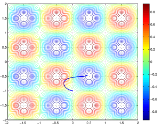
Figure 1: Potential energy surface for the 2-dimensional toy problem showing the evolution (solid blue line) of the system from a metastable state to an index-1 saddle point by following (2).

The stochastic version of GAD can be used to navigate the PES to sample different saddle points. Fig. 2 shows the results for stochastic dynamics performed by the system on the PES. The system spends majority of its time around saddle points in contrast to general overdamped Langevin dynamics in which the system samples stable fixed points of the PES.

Next, we turn to MD-GAD prescribed in (5). In Fig. 2 the system travels from the initial locally stable fixed point at ($\frac{1}{2},-\frac{1}{2}$) to the final metastable state at ($\frac{9}{2},-\frac{9}{2}$) by passing through many saddle points and locally stable fixed points. The simulation is started with zero kinetic energy. As the system walks out of the initial energy well and moves towards the saddle point, the KE of the system increases and attains a maximum value. This pushes the system towards the next metastable point where the KE reduces to zero. Subsequently, the system again gains kinetic energy as it moves close to the next saddle point. As this process is repeated many fixed points of the PES are sampled.

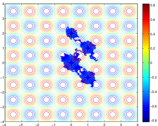
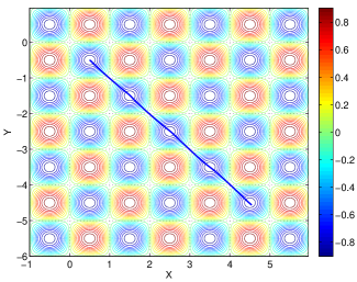
Figure 2: 2 Solutions of (4) showing the trajectory followed by a system on the 2-dimensional PES. The system spends majority of its time near saddle points. 2 Shows the evolution of the system using MD-GAD prescribed in (5). In this case the system can easily traverse through many locally stable and index-1 saddle points of $V\left(x,y\right)$.

III Applications

To further illustrate our approach, we simulate an ensemble of saddle points for two systems: (a) a heptamer island on $(111)$ surface of copper and (b) a surface vacancy and ad-atom pair on the $(111)$ surface of copper. The heptamer island system has been widely studied by Henkelman et al. using the dimer method and most recently by J$\rm\ddot{o}$nsson et al. to benchmark the convergence of different saddle point finding strategies.Henkelman and Jonsson (1999); Miron and Fichthorn (2001); Pedersen et al. (2011) The second example has clear time-scale separation between different rare events, namely, ad-atom diffusion and vacancy diffusion and hence presents excellent opportunity to test the scope of saddle point finding algorithms. While diffusion of an ad-atom on a metal surface has been studied before the presence of a vacancy adds significant complexity to the problem.Miron and Fichthorn (2001); Pedersen et al. (2011) Our intention is to explore the high dimensional PES close to these locally stable configurations to probe and catalogue some of the probable surface activity that can play an important role in other scenarios where quantitative analysis of different rare events may be difficult.

III.1 Selecting an “active region” of the sample

The problem of determining saddle points close to a local minimum entails moving out of the potential energy well along preferential directions in the multidimensional configuration space. The challenge in sampling these preferential directions comes from the fact that they represent only a miniscule fraction of all the possible directions emanating from the initial locally stable fixed point on the high dimensional PES.

Our aim is to significantly reduce the size of the configuration space by selecting a small, yet important, region of the sample. In materials physics, many deformation processes can be easily traced by analyzing the softest eigenmodes of the Hessian. This helps in determining a vulnerable region of the system. In systems where one has an intuitive understanding of the vulnerable region ($\Omega_{v}$) one can select a set of atoms and include their first nearest neighbors to form a set of “active region” $\Omega$, such that $\Omega_{v}\subset\Omega$. We show that a more prudent way to sample $\Omega_{v}$, which is prone to deformation, is by analyzing the unit force vector close to the initial locally stable configuration. Once the vulnerable DOF are identified, the corresponding atoms and their first nearest neighbors are selected to form the “active region” of the sample. Our assumption is that this “active region” corresponds to a significantly reduced configuration space where probable low barrier transition events can take place.

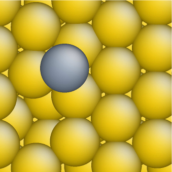
Figure 3: Local minimum configuration for the system containing a surface vacancy and an ad-atom (shown in grey) on (111) surface of a copper thin film.

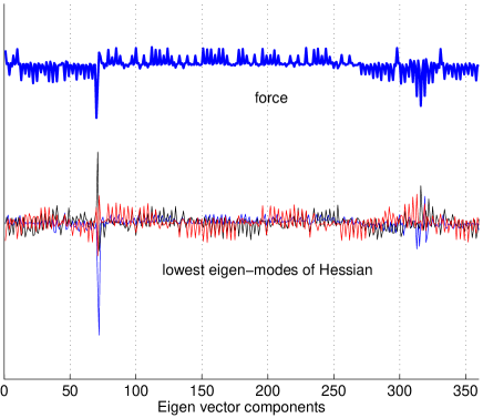
Figure 4: 4 Shows the eigenvalues of the Hessian, arranged in ascending order, at the local minimum configuration for the vacancy ad-atom system. The upper inset shows that the Hessian is diagonal dominant and the lower inset shows the clustering of low lying eigenvalues of the Hessian. 4 Shows the different DOF of the unit force vector (blue) and the superposition of 6 lowest eigenvectors of the Hessian at the local minimum configuration. The vulnerable DOF can be easily isolated.

Let us consider the system containing a surface vacancy and an ad-atom on the $(111)$ surface of a copper thin film (Fig. 3). For this system, we have explicitly evaluated Hessian for the relaxed initial configuration (force norm $<10^{-4}$ eV/$\rm\AA$). The elements in the $i$-th row of the Hessian matrix are determined by displacing the $i$-th DOF by a small displacement $\delta x_{i}$ from the equilibrium structure and evaluating the change in the force on all atoms. The Hessian (characterized by the upper inset in Fig. 4) is then diagonalized and its eigenvalues calculated. Fig. 4 shows the spectrum of the Hessian of the system. The lower inset in the figure shows the clustering of low-lying eigenvalues which may be difficult to resolve by using power method based tools. A superposition of the low-lying eigenvectors (first 6 lowest eigenvectors, neglecting the global rotation and global translation components) are plotted in Fig. 4.

Fig. 4 also shows the contributions of the different DOF to the unit force vector (shown in blue) at the initial locally stable fixed point of the energy landscape. Upon comparison with the superposition of the six low-lying eigenvectors, we find the the DOFs that have significantly higher weights in the unit force vector also correspond to those in the low lying eigenvectors of the Hessian. This suggest that close to a locally stable fixed point the force can provide information about the vulnerable DOF of the system and can be used to obtain probable initial direction vectors for probing saddle points on the PES. Following the above argument, using the unit normed force at the local minimum point, we selected a set of 23 atoms as our “active region” $\Omega$.

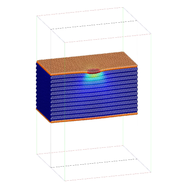
Figure 5: Simulation cell set-up for nanoindentation on (111) surface of an initially defect-free Cu thin-film containing 112,320 atoms. 5 shows a cross section of the system after indentation performed using a spherical smooth indenter of radius 25 $\rm\AA$ on the (111) free surface. The indentation direction is perpendicular to the (111) surface. The atoms have been colored by their shear strain (dark blue corresponds to zero strain and red corresponds to maximum shear strain $\sim 0.20$). 5 shows the contributions from different DOF to the unit force thus showing the atoms vulnerable to deformation. The inset shows a magnified portion of the plot. The vulnerable DOF can be easily identified.

We find that even for complicated non-equilibrium processes involving many potential transition events in presence of external fields (such as stress, etc.) the unit force on the system can be very informative. To illustrate this we use the example of nanoindentation. Fig. 5 shows a representative system containing 112,320 copper atoms. The simulation cell has lattice vectors along $[1\bar{1}0]$, $[111]$ and $[11\bar{2}]$ directions. While free surface conditions are prevalent along $[111]$ direction, periodic boundary conditions are imposed along the perpendicular directions. The system is elastically indented using a smooth spherical indenter (radius 25 $\rm\AA$), imposed by a force field, to an indentation depth of 4.19 $\rm\AA$. After indentation, constrained minimization (force norm $<10^{-2}$ eV/$\rm\AA$) is performed to obtain a locally stable configuration. Fig. 5 shows the contributions of the different DOF in the unit force vector from which we can easily select $\Omega$. Analysis of the probable transition events taking place during nanoindentation will be presented elsewhere.

III.2 Initial direction vectors

Since the overall system size corresponds to a large configuration space, an activated region of the sample is selected following a procedure described in the previous section. From the set of atoms within $\Omega$, we obtain a set of initial direction vectors by the following procedure : select $m$ atoms and randomly initializing the 3$m$ direction components while keeping the remaining components of the direction vector equal to zero. The set of $m$ atoms is selected by picking an atom $i$ and its ($m-1$) nearest neighbors from $\Omega$. If the atom $i$ has $n$ ($<m-1$) nearest neighbors inside $\Omega$ then the direction has only ($3n+3$) randomly initialized components and the remaining DOF are set to zero. For our study of rare events in the representative systems described earlier we use $m$ = 1, 2, 4, 12, though one can resort to a different set of values.

Our choice of selectively activating only a few components of the direction vector stems from the fact that even though physical processes, such as different deformation mechanisms, taking place in most materials have activation volumes in the range of 0.1$b^{3}$-1000$b^{3}$, $b$ is the Burgers vector of the system, the size of the nucleus in the initial stages can be quite small. A smaller activation volume corresponds to a localized process involving only few atoms such as interstitial diffusion, vacancy diffusion etc., while a larger activation volume corresponds to a process which is more delocalized, such as, forest hardening, Orowan loopin, etc.Dao et al. (2007) In each of these processes, since only a few degrees of freedom of the direction vector are explored, ideally one needs humongous number of randomly initialized vectors to sample majority of the most probable rare events. Our proposed selection procedure overcomes this sampling problem.

III.3 Convergence criteria

Once a set of the desired direction vectors is obtained, one can move out of basins of attraction by moving along these directions. GAD guarantees that the system converges to an index-1 saddle point on the energy surface. However, the convergence will depend on how fast the system can relax to the lowest eigenmode in the vicinity of the saddle point. During this time it is possible that the system might have traversed through few different fixed points on the PES. In order to avoid this “overshooting” one might resort to a smaller time step. However, this is not conducive as the majority of initialized direction vectors have sufficient time to relax to the minimum eigenmode much before the system reaches the separatrix.

Hence, a pragmatic approach is needed to determine whether the system has left the basin of attraction or not. Our approach is motivated by the existence of an unique equilibrium bond length ($r_{\rm o}$) between nearest neighbor atoms in a locally stable configuration. A rare event involves a process of bond-breaking between nearest neighbors (which corresponds to a bond length, $r$) in the group of atoms taking part in the process. This criteria can be used to identify the approach of a system to a saddle point. We use the ratio $q=\left(r-r_{\rm o}\right)/r_{\rm o}$ for this purpose. To sample saddle points close to a local minimum, suggested values of $q_{c}$ lie in the range $\sim 0.30-0.40$.Miron and Fichthorn (2003, 2004) Using this criteria has an added flexibility : one can selectively tune $q_{c}$ to determine a distribution of saddle points within a given distance from the initial configuration in the hyper-space.

For the sampling saddle points in the representative examples we use $q_{c}$ = 0.50. The system follows (2) with $\gamma=1$ for $q\leq q_{c}$. To identify any bond breaking event, $q$ is calculated every 10 steps. Once, $q>q_{c}$ we use $\gamma=0.25$ and for each evolution step of $\bf x$, the direction vector $\bf n$ is evolved 2 times to converge to the minimum eigenmode.

III.4 Surface vacancy ad-atom pair on (111) surface of cooper

The simulation setup consists of a, 480 Cu atoms, simulation cell with axis vectors along $[110]$, $[1\bar{1}1]$ and $[\bar{1}12]$ directions. The set up consists of 6 $(111)$ planes stacked on top of each other with periodic boundary conditions imposed along $[110]$ and $[\bar{1}12]$ directions while free surface conditions maintained along $[1\bar{1}1]$ direction. On atom is removed from the surface to form a surface vacancy and placed on a vacant fcc site close to the vacancy to form an ad-atom. Fig. 3 shows the initial configuration obtained by local minimization to a force of 10^-4 eV/$\rm\AA$. The ad-atom is shown in grey. Fig. 4 shows the weights of different DOF in the unit normed force vector for the initial configuration. The vulnerable DOF are easily identifiable. These DOF are used to generate 661 initial direction vectors.

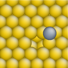
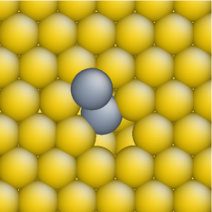
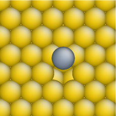
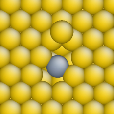
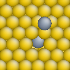
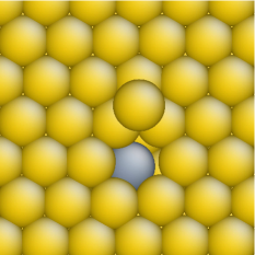
Figure 6: Some converged saddle configurations for the vacancy ad-atom system obtained from GAD simulations. 6 ad-atom diffusion (barrier 0.01 eV), 6 collective process involving ad-atom and vacancy migration (barrier 0.15 eV), 6 vacancy ad-atom annihilation (barrier 0.30 eV), 6 vacancy diffusion (barrier 0.59 eV), 6 sub-surface vacancy formation (barrier 0.77 eV), 6 sub-surface vacancy formation (barrier 0.82 eV). Some of the structures are shifted in plane for proper viewing.

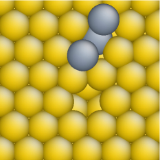
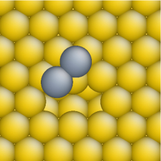
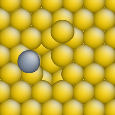
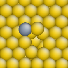
Figure 7: Some converged saddle configurations for the vacancy ad-atom system obtained from GAD simulations. 7 ad-atom formation by exchange mechanism (barrier 1.14 eV), 7 divacancy and ad-atom formation (barrier 1.40 eV), 7 divacancy and ad-atom formation (barrier 1.81 eV), 7 bulk-vacancy and ad-atom formation (barrier 2.08 eV).

Fig. 6 to Fig. 7 shows the probable transition events with increasing activation energy barriers. The smallest barrier (0.01 eV) corresponds to an ad-atom diffusion. The difference in energy between a fcc and hcp site on a free surface is much smaller than that in metals like Pt, resulting in a significantly smaller ad-atom diffusion barrier. We found the process of diffusion of both ad-atom and vacancy in a concerted way, as shown in Fig. 6 has a little higher barrier of 0.15 eV. The other significant events are ad-atom diffusion to annihilate the ad-atom and surface vacancy pair (Fig. 6), vacancy diffusion on the surface (Fig. 6) and sub-surface vacancy formation ( Fig. 6 and 6). Fig. 7 corresponds to ad-atom migration by exchange process. Some of the transition events are affected by the location of ad-atom and vacancy. For example, as shown in Fig. 7 and Fig. 7, the formation of a divacancy and a nearest-neighbor ad-atom pair has lower barrier than formation of a divacancy and two ad-atoms. Fig. 7 corresponds to formation of a bulk vacancy and an ad-atom.

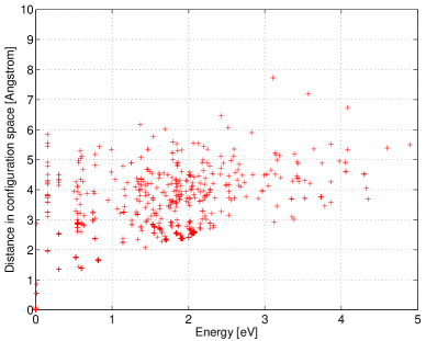
Figure 8: Summary of results depicting a wide spectrum of converged energy barriers for different rare events as a function of the distance of the final saddle configuration from the initial locally stable configuration for the surface vacancy and ad-atom system. The results correspond to simulations performed with $q_{c}=0.50$ thus allowing the possibility of sampling a much larger portion of the configuration space for index-1 saddle points.

Fig. 8 shows a summary of the results obtained from converged GAD simulations. The results are depicted as the distribution of the converged saddle energies as a function of distance of the converged saddle configuration from the initial configuration in the configuration space. As can be seen from the figure, there are multiple saddle configurations with same energy but separated by a finite distance in the configuration space.

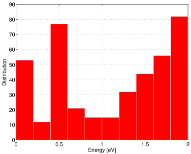
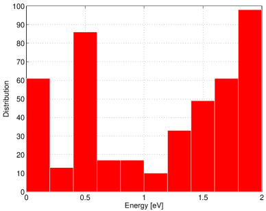
Figure 9: Summary of results depicting the distribution of converged saddle energies (with respect to the initial structure) for $q_{c}=0.40$ (9) and $q_{c}=0.30$ (9) for the system with a surface vacancy and ad-atom. The results correspond to the evolution equations (2)

Fig. 9 shows the distribution of converged saddle energies less than 2.0 eV for different values of $q_{c}$ for a fixed set of initial direction vectors. This suggests that, for a sufficiently large set of well sampled direction vectors, the values of $q_{c}$ in the range of 0.30-0.50 provides a good collection of low barrier saddle points. Though our selection of initial direction vectors significantly decreases repeated visits of the same saddle point, however on a high dimensional PES there exists saddle points with similar barriers but separated by a finite distance. The above results have significant contributions from such scenarios.

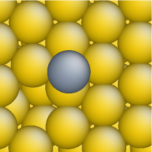
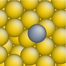
Figure 10: Sampling of saddle points using MD-GAD. The adatom (shown in grey) in this case hops between different index-1 saddle points (Fig. $\ref{AdatomMigration2}-\ref{AdatomMigration4}$) on the $\langle 111\rangle$ surface of Cu. Fig. 10 is the initial structure.

Fig. 10 shows a collection of saddle points obtained by using MD-GAD. In this case, the simulations are started with zero initial velocity from the local minimum in Fig. 10 and the direction vector preferentially initialized to activate the ad-atom. As the simulation progresses, the system moves from the local minimum point to a saddle point (Fig. 10) where the KE reaches a maximum value. Then the high KE pushes the system to the next saddle point shown in Fig. 10. Thus MD-GAD effectively samples many low lying saddle points on the PES.

III.5 Heptamer island on (111) surface of copper

The simulation setup consists of a sample with 487 Cu atoms and lattice vectors parallel to $[110]$, $[1\bar{1}1]$ and $[\bar{1}12]$ directions. The periodic boundary conditions are imposed along $[110]$ and $[\bar{1}12]$ while free surface conditions are maintained along $[1\bar{1}1]$ direction. The atomic interactions are modeled using an EAM potential developed by Mishin et al.Mishin et al. (1999) Initially all atoms in the seven atom heptamer island occupy fcc sites on the $(111)$ surface.

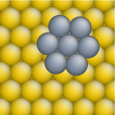
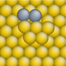
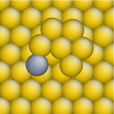
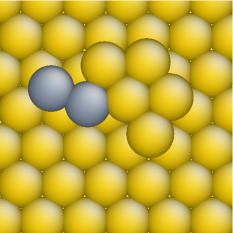
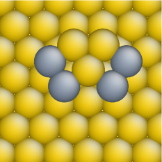
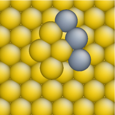
Figure 11: Some converged saddle configurations for the vacancy ad-atom configuration obtained from GAD simulations. 11 island sliding on (111) surface (barrier 0.39 eV), 11 two atom sliding (barrier 0.49 eV), 11 single atom hopping (barrier 0.683), 11 two atom sliding (barrier 0.69 eV), 11 two atom sliding process taking place at two locations on the island (barrier 0.78 eV), 11 sliding of atoms (barrier 0.84 eV).

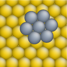
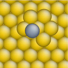
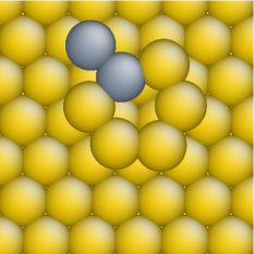
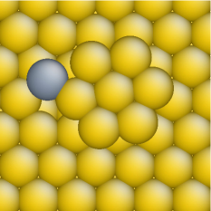
Figure 12: Some converged saddle configurations for the vacancy ad-atom configuration obtained from GAD simulations. 12 island rotation (barrier 0.92 eV), 12 ad-atom formation on heptamer island (barrier 1.39 eV), 12 two atom sliding process (barrier 1.49 eV), 12 ad-atom and surface vacancy formation (barrier 1.86 eV).

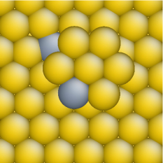
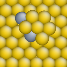
Figure 13: 13 ad-atom formation by exchange mechanism which changes the shape of the heptamer island (barrier 1.84 eV).

Fig. 11 to Fig. 12 shows a collection of, low barrier, saddle configurations. From our simulations, we find many collective processes, such as those involving lateral translation (energy barrier 0.39 eV) and rotation (energy barrier 0.92 eV) of the heptamer island. These collective processes have also been reported for islands of different sizes and shapes.Miron and Fichthorn (2001) Other low barrier events include sliding of two nearest neighbor atoms belonging to the heptamer island (Figs. 11, 11, 11 and 12) all with barriers 0.49-0.69 eV. Fig. 11 involves a cooperative rearrangement and sliding of three atoms and has little higher barrier. The sliding of group of atoms with respect to others in the island resembles the process of formation of a dislocation in a bulk crystal. We also observe movement of an island by repeated shearing of different layers.Miron and Fichthorn (2001) Fig. 13 and 12 shows different ways of formation of a surface vacancy and an ad-atom. While the process in Fig. 12 involves a surface atom hopping out of plane to attach itself to the island the process in Fig.13 involves a cooperative “exchange” mechanism involving a sub-surface atom.Pedersen et al. (2011)

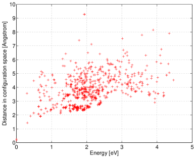
Figure 14: Summary of results depicting a wide spectrum of converged energy barriers for different rare events as a function of the distance of the final saddle configuration from the initial locally stable configuration for the system with a heptamer island on $(111)$ surface.

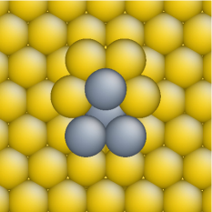
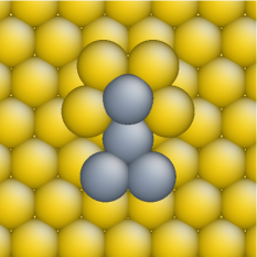
Figure 15: Snapshots of the collective process of formation of a sub-surface vacancy and an ad-atom on top of the heptamer island. The atoms involved in the process are shown in grey (barrier 2.42 eV).

Fig. 14 shows a summary of the converged saddle configuration energies, obtained using the 843 initial direction vectors, as a function of the distance in the configuration space from the initial local minimum configuration. Setting the parameter $q_{c}=0.50$ provides the flexibility to sample a larger portion of the configuration space near the initial configuration. This also allows us to capture events which involve multiple saddle points thus providing vital information about possible channels for probable transition events. Fig. 15 shows one such example where a sequence of transition events leads to the formation of a bulk vacancy, an ad-atom on top of the heptamer island and subsequent change in shape of the island on the $(111)$ surface.

IV Conclusions

We have shown that the deterministic, molecular dynamics or stochastic versions of GAD can be used as effective tools for sampling saddle points on the PES. The algorithms presented here are scalable to systems of higher dimensions. The computational cost and memory requirements are similar to molecular dynamics simulations.

A method to initialize the direction vectors along which the system can move out of the initial potential energy well is described. It is based on the knowledge of the vulnerable DOF of the system from the force at initial local minimum. All the operations in GAD and its finite temperature variants have $\mathcal{O}\left(N\right)$ ($N$ is the number of DOF) computational complexity. Our use of a criteria based on equilibrium bond length of atoms in a system to identify the closeness of a system from the initial local minimum point also saves computational cost.

The finite temperature versions of GAD open avenues for sampling of saddle points on the PES. Generally existing macroscopic models are based on information obtained from locally stable fixed points of a system. In the stochastic version of GAD, since the system can hop between different low energy saddle points, a wealth of information can be obtain about the saddle configurations. This information can then be used to improve the existing mean field models.

GAD can be extended to handle higher index saddle points, as was done in Ref[15]. It is obvious that one can also extend the work presented to those cases.

Our results for point defect activity on a $(111)$ surface obtained from GAD show a variety of processes involving more than a single atom. Indeed the wide spectrum of diffusion processes revealed by GAD for ad-atoms, vacancies and islands can provide much needed insight into the probable mechanisms behind many experimentally observed surface phenomena.Tsong and Chen (1992); Ferron et al. (2004); van Gastel et al. (2001); Montalenti et al. (2002)

V Appendix I:Local convergence analysis for MD-GAD

The fixed points of PES are also the fixed points of (5). To see this consider a two dimensional system with force ${\bf F}=f_{x}\hat{i}+f_{y}\hat{j}$ and direction vector ${\bf n}=n_{x}\hat{i}+n_{y}\hat{j}$, where $f_{x}$, $f_{y}$ and $n_{x}$, $n_{y}$ are individual components of force and direction vectors, respectively, along the $i$ and $j$ axis. Consequently, the solutions of $\dot{\bf v}=0$ are:

$$f_{x}\hat{i}+f_{y}\hat{j}=2\lambda\left(n_{x}\hat{i}+n_{y}\hat{j}\right),\qquad\lambda=f_{x}n_{x}+f_{y}n_{y}\;,\qquad n_{x}^{2}+n_{y}^{2}=1$$ (9)

Equating the individual vector components on both sides of the above equation we obtain

$$\left.\begin{array}[]{cc}f_{x}\left(n_{y}^{2}-n_{x}^{2}\right)&=2f_{y}n_{y}n_{x}\\ f_{y}\left(n_{x}^{2}-n_{y}^{2}\right)&=2f_{x}n_{y}n_{x}\\ \end{array}\;\right\}\qquad f_{x}^{2}+f_{y}^{2}=0$$ (10)

which is possible only if individual components of the force vector are zero. So for all values of the direction vector the above condition is satisfied only at fixed points of $V\left(\bf x\right)$.

The Jacobian matrix of MD-GAD has the form :

$$\tilde{\bf J}_{1}=\left[\begin{array}[]{ccc}0&\mathbb{I}&0\\ \left(\bf J-2nn^{\rm T}J\right)&0&-2\left({\bf F^{\rm T}n}\mathbb{I}+{\bf nF}^{\rm T}\right)\\ \bf L&0&\left(\bf J-{2}nn^{\rm T}J-n^{\rm T}Jn\mathbb{I}\right)\end{array}\right]$$ (11)

where,$\;\bf L$ is a $n\times n$ matrix involving the third order derivatives of $V$. At any fixed point of the potential, since the derivative of $V$ is zero, the term ${\bf F^{\rm T}n}\mathbb{I}+{\bf nF}^{\rm T}$ is zero and the eigenvalues of $\tilde{\bf J}_{1}$ at these fixed points can be obtained from

$$\tilde{\bf J}_{1}=\left[\begin{array}[]{ccc}0&\mathbb{I}&0\\ \left(\bf J-2nn^{\rm T}J\right)&0&0\\ \bf L&0&\left(\bf J-2nn^{\rm T}J-n^{\rm T}Jn\mathbb{I}\right)\end{array}\right]$$ (12)

This means, eigenvalues of $\tilde{\bf J}_{1}$ can be obtained from the eigenvalues of $\bf N=\left(\bf J-n^{T}Jn\mathbb{I}-2nn^{\rm T}J\right)$ and square root of the eigenvalues of $\bf M=\left(\bf J-2nn^{\rm T}J\right)$.

Let $\lambda_{1}\left(\bf x\right)\leq\lambda_{2}\left(\bf x\right)\leq\lambda_{3}\left(\bf x\right)\leq...\leq\lambda_{n}\left(\bf x\right)$ be the eigenvalues (including degeneracies) of $\bf H\left(\bf x\right)$ and $\left({\bf w}_{1},{\bf w}_{2},...,{\bf w}_{n}\right)$ be the associated set of orthonormal eigenvectors at some fixed point of $V$. A negative (positive) eigenvalue of $\bf J$ (Hessian) corresponds to a stable manifold, while a positive eigenvalue of $\bf J$ corresponds to an unstable manifold. Assuming $\bf n$ equals ${\bf w}_{1}$ (i.e. the minimum eigen mode of the local Hessian), we find that

$${\bf Mw}_{i}=\left(\bf J-2nn^{\rm T}J\right){\bf w}_{i}=-\lambda_{i}{\bf w}_{i}+2\lambda_{1}\delta_{i1}{\bf w}_{i}$$ (13)

$${\bf Nw}_{i}=\left(\bf J-n^{T}Jn\mathbb{I}-2nn^{\rm T}J\right){\bf w}_{i}=-\lambda_{i}{\bf w}_{i}+\lambda_{1}{\bf w}_{i}+2\lambda_{i}\delta_{i1}{\bf w}_{i}$$ (14)

Thus, the eigenvalues of $\tilde{\bf J}_{1}$ are $\{\sqrt{\lambda_{1}},-\sqrt{\lambda_{1}},2\lambda_{1}\}$ for $i=1$ and $\{\sqrt{-\lambda_{i}},-\sqrt{-\lambda_{i}},\left(\lambda_{1}-\lambda_{i}\right)\}$ when ${\bf w}_{i}\perp{\bf w}_{1}$ (i.e. $i>1$). At an index-1 saddle point $\lambda_{1}<0$ and $\lambda_{i}>0$ for all $i>1$. Consequently, the eigenvalues of $\tilde{\bf J}_{1}$ are all negative or complex numbers and this fixed point of $V\left(\bf x\right)$ becomes linearly stable attractor for the dynamical system (2).

At a locally stable fixed point of $V\left(\bf x\right)$ all the eigenvalues of $\bf H$ are positive. Thus, $\tilde{\bf J}_{1}$ has two positive eigenvalues, $n$ negative eigenvalues and ($2n-2$) complex eigenvalues. Correspondingly, there exists two unstable manifolds due to which this fixed point becomes unstable in MD-GAD. Detailed analysis of convergence of GAD to index-1 saddle points for non-gradient systems has been reported elsewhere.E and Zhou (2011)

Now, for the dynamical system (2) the Jacobian near a fixed point of $V\left(\bf x\right)$ is given by

$$\tilde{\bf J}_{2}=\left[\begin{array}[]{cc}\left(\bf J-2nn^{\rm T}J\right)&0\\ {\bf L}&\left(\bf J-{2}nn^{\rm T}J-n^{\rm T}Jn\mathbb{I}\right)\\ \end{array}\right]$$ (15)

Following a similar procedure, the eigenvalues of the $\tilde{\bf J}_{2}$ are given by the eigenvalues of $\bf N$ and $\bf M$. We find that all the eigenvalue of $\tilde{\bf J}_{2}$ are negative at index-1 saddle point of $V\left(\bf x\right)$. In contrast, there exists two positive and (2$n$-2) negative eigenvalues of $\tilde{\bf J}_{2}$ at a stable fixed point of $V\left(\bf x\right)$. Thus local minimum points of $V\left(\bf x\right)$ are linearly unstable while index-1 saddle points become locally stable attractors.

VI Appendix II:Local convergence analysis for ART

Having analyzed the stability of different fixed points of $V\left(\bf x\right)$ within GAD, let us try to analyze the stability of fixed points on $V\left(\bf x\right)$ in ART. Originally, ART was proposed to explore the PES and only in subsequent modified versions it converges to a saddle point.Cancès et al. (2009); Marinica et al. (2011) Here we evaluate the propensity of ART to visit an index-1 saddle point while exploring the PES.

In ART, the system evolves by the following equation:

$$\bf\dot{x}=\bf F\left(\bf x\right)-\nu\left({\bf F}\left(\bf x\right),\bf n\right)n,\qquad\nu>1\\$$ (16)

where, $\bf n$ is the direction vector given by the difference of the current location $\bf x$ and initial location $\bf x_{o}$ in the configuration space, i.e. $\bf n=\left(\bf x-x_{o}\right)/\left|\bf x-x_{o}\right|$. Close to a fixed point of $V\left(\bf x\right)$ since the force is zero, the Jacobian, $\tilde{\bf J}_{3}$, for (16) is $\tilde{\bf J}_{3}=\left(\bf J-\nu nn^{\rm T}J\right)$ where, ${\bf J}=-{\bf H}=-\nabla^{2}V\left(\bf x\right)$. To illustrate the stability of the dynamical system in (16), let us consider for example a simple 2D potential energy landscape :

$$V\left(x,y\right)=\sin\left(\pi x\right)\sin\left(\pi y\right).$$ (17)

At a saddle point, for instance at ($0,0$), the Hessian has eigenvalues $\{1,-1\}$. Assuming ${\bf n}=\left[n_{1}\;\;n_{2}\right]^{\rm T}$, with $n^{2}_{1}+n^{2}_{2}=1$, the Jacobian of ART at a fixed point of $V\left(\bf x\right)$ is

$$\tilde{\bf J}_{3}=\left(\left[\begin{array}[]{cc}1&0\\ 0&1\end{array}\right]-\nu\left[\begin{array}[]{cc}n^{2}_{1}&n_{1}n_{2}\\ n_{1}n_{2}&n^{2}_{2}\end{array}\right]\right)\bf J$$ (18)

At ($0,0$), if $\bf J$ is given by

$$\bf J=\left[\begin{array}[]{cc}-1&0\\ 0&1\end{array}\right],\quad\Rightarrow\;\tilde{\bf J}_{3}=\left[\begin{array}[]{cc}\left(1-\nu n^{2}_{1}\right)&-\nu n_{1}n_{2}\\ \nu n_{1}n_{2}&\left(1-\nu n^{2}_{2}\right)\end{array}\right]$$ (19)

Diagonalizing $\tilde{\bf J}_{3}$, we obtain the following eigenvalues

$$\left\{\frac{\left(2-\nu\right)}{2}-\frac{\nu}{2}\sqrt{\left(1-8n^{2}_{1}n^{2}_{2}\right)}\;,\;\frac{\left(2-\nu\right)}{2}+\frac{\nu}{2}\sqrt{\left(1-8n^{2}_{1}n^{2}_{2}\right)}\;\right\}$$ (20)

Since, $1=\left(n^{2}_{1}+n^{2}_{2}\right)^{2}\geq 4n^{2}_{1}n^{2}_{2}\;\Rightarrow n^{2}_{1}n^{2}_{2}\leq 1/4$, consequently $\left(1-8n^{2}_{1}n^{2}_{2}\right)\geq-1$. Thus, depending on the direction vector $\bf n$ the saddle can be stable or unstable for the dynamical equation in (16).

References

- Eyring (1935) H. Eyring, J. Chem. Phys. 3, 107 (1935).
- Hanggi et al. (1990) P. Hanggi, P. Talkner, and M. Borkovec, Reviews Of Modern Physics 62, 251 (1990).
- Fecht (1992) H. J. Fecht, Nature 356, 133 (1992).
- Crippen and Scheraga (1971) G. M. Crippen and H. A. Scheraga, Archives Of Biochemistry And Biophysics 144, 462 (1971).
- Barkema and Mousseau (1996) G. T. Barkema and N. Mousseau, Physical Review Letters 77, 4358 (1996).
- Pedersen et al. (2011) A. Pedersen, S. F. Hafstein, and H. Jonsson, SIAM Journal of Scientific Computing 33, 633 (2011).
- Cerjan and Miller (1981) C. J. Cerjan and W. H. Miller, Journal Of Chemical Physics 75, 2800 (1981).
- Henkelman and Jonsson (1999) G. Henkelman and H. Jonsson, Journal Of Chemical Physics 111, 7010 (1999).
- Olsen et al. (2004) R. A. Olsen, G. J. Kroes, G. Henkelman, A. Arnaldsson, and H. Jonsson, Journal Of Chemical Physics 121, 9776 (2004).
- Poddey and Blochl (2008) A. Poddey and P. E. Blochl, Journal Of Chemical Physics 128, 44107 (2008).
- Munro and Wales (1999) L. J. Munro and D. J. Wales, Physical Review B 59, 3969 (1999).
- Mousseau and Barkema (2000) N. Mousseau and G. T. Barkema, Physical Review B 61, 1898 (2000).
- Cancès et al. (2009) E. Cancès, F. Legoll, M. C. Marinica, K. Minoukadeh, and F. Willaime, Journal Of Chemical Physics 130, 114711 (2009).
- Marinica et al. (2011) M. . C. . Marinica, F. . Willaime, and N. . Mousseau, Physical Review B 83, 094119 (2011).
- E and Zhou (2011) W. E and X. Zhou, Nonlinearity 24, 1831 (2011).
- Nose (1984) S. Nose, Journal Of Chemical Physics 81, 511 (1984).
- Hoover (1985) W. G. Hoover, Physical Review A 31, 1695 (1985).
- Parrinello and Rahman (1980) M. Parrinello and A. Rahman, Physical Review Letters 45, 1196 (1980).
- Parrinello and Rahman (1981) M. Parrinello and A. Rahman, Journal Of Applied Physics 52, 7182 (1981).
- Miron and Fichthorn (2001) R. A. Miron and K. A. Fichthorn, Journal Of Chemical Physics 115, 8742 (2001).
- Dao et al. (2007) M. Dao, L. Lu, R. J. Asaro, J. T. M. De Hosson, and E. Ma, Acta Materialia 55, 4041 (2007).
- Miron and Fichthorn (2003) R. A. Miron and K. A. Fichthorn, Journal Of Chemical Physics 119, 6210 (2003).
- Miron and Fichthorn (2004) R. A. Miron and K. A. Fichthorn, Physical Review Letters 93 (2004).
- Mishin et al. (1999) Y. Mishin, D. Farkas, M. J. Mehl, and D. A. Papaconstantopoulos, Physical Review B 59, 3393 (1999).
- Tsong and Chen (1992) T. T. Tsong and C. L. Chen, Nature 355, 328 (1992).
- Ferron et al. (2004) J. Ferron, L. Gomez, J. J. de Miguel, and R. Miranda, Physical Review Letters 93, 166017 (2004).
- van Gastel et al. (2001) R. van Gastel, E. Somfai, S. B. van Albada, W. van Saarloos, and J. W. M. Frenken, Physical Review Letters 86, 1562 (2001).
- Montalenti et al. (2002) F. Montalenti, A. F. Voter, and R. Ferrando, Physical Review B 66, 205404 (2002).