The absolute positive partial transpose property
for random induced states

Abstract.

In this paper, we first obtain an algebraic formula for the moments of a centered Wishart matrix, and apply it to obtain new convergence results in the large dimension limit when both parameters of the distribution tend to infinity at different speeds.

We use this result to investigate APPT (absolute positive partial transpose) quantum states. We show that the threshold for a bipartite random induced state on $\mathbf{C}^{d}=\mathbf{C}^{d_{1}}\otimes\mathbf{C}^{d_{2}}$, obtained by partial tracing a random pure state on $\mathbf{C}^{d}\otimes\mathbf{C}^{s}$, being APPT occurs if the environmental dimension $s$ is of order $s_{0}=\min(d_{1},d_{2})^{3}\max(d_{1},d_{2})$. That is, when $s\geqslant Cs_{0}$, such a random induced state is APPT with large probability, while such a random states is not APPT with large probability when $s\leqslant cs_{0}$. Besides, we compute effectively $C$ and $c$ and show that it is possible to replace them by the same sharp transition constant when $\min(d_{1},d_{2})^{2}\ll d$.

1. Introduction

Geometry of quantum states strives to understand the geometric properties of subsets of quantum states, and has attracted considerable attention, especially in the case of the large dimension [2, 3, 15, 35, 37, 38, 41, 42]. The high dimensional setting is common (and of particular interest) in Quantum Information Theory whose building blocks, quantum states, often are objects with huge dimension (for instance, the set of quantum states on the system $(\mathbf{C}^{3})^{\otimes 8}$ has dimension 43046720). This high dimensional setting indicates the importance of random constructions which now is a main tool in understanding the typical behavior of random induced states. To generate random induced states, one often relies on random matrices. The connections between Random Matrices and Quantum Information Theory were pushed forward by Hayden, Leung, and Winter in their studies of aspects of generic entanglement [19]. Together with tools from Geometric Functional Analysis and Convex Geometric Analysis, random matrices and random constructions have led to many important (and even unexpected) results, such as Hastings’s disproof of the famous additivity conjecture for the classical capacity of quantum channels [18]. Recent contributions include the studies of the generic properties for entanglement vs. separability, and PPT (positive partial transpose) vs non-PPT [1, 4, 5, 10].

Detecting quantum entanglement, a phenomenon first discovered in [13] and now being the key ingredient of quantum algorithms (see [27, 32]), is one of the fundamental problems in Quantum Information Theory. Among those necessary and/or sufficient conditions for separability and entanglement, the Peres-Horodecki PPT criterion [22, 30] is the simplest but the most powerful one. The Peres-Horodecki PPT criterion is a necessary condition and is sufficient only for the systems $\mathbf{C}^{2}\otimes\mathbf{C}^{2}$ and $\mathbf{C}^{2}\otimes\mathbf{C}^{3}$ [34, 40]. From the computational complexity point of view, separability and PPT are quite different: determining separability is an NP-hard problem [16], but determining PPT is easy since it only requires to verify the eigenvalues of the partial transpose of given states being positive. Note that both the separability and PPT are encoded in the spectral properties of quantum states in a complicate way. Necessary and/or sufficient conditions on determining separability and PPT by just the information of eigenvalues (referred to as the absolute separability and absolute PPT in literature) could be very useful in Quantum Information Theory as it can help to reduce the cost of storage spaces and (processing) time. For absolute separability, less results are known; however, necessary and sufficient conditions for APPT have been found by Hildebrand [20]. Understanding when a random induced states is APPT is the main motivation of this work.

To that end, we first prove that a properly centered $d\times d$ Wishart matrix of parameter $s$ has its expected normalized moments that can be written as a polynomial in the variables $d$ and $d/s$. The coefficients of this polynomial have a simple combinatorial interpretation, and some families of coefficients are known. This algebraic fact has important consequences in the two parameter asymptotic study of the Wishart matrix. Indeed, it allows in particular to capture the precise nature of the behavior of the Wishart matrix in the case where $d\to\infty$, and in particular in the case where $s/d\to\infty$ too. We summarize our first main result as follows:

Theorem A. Let $W_{d}$ be a $d\times d$ Wishart matrix of parameter $s$ and let $Z_{d}=\sqrt{ds}\left(\frac{W_{d}}{ds}-\frac{\mathbb{Id}}{d}\right)$ be its centered and renormalized version. The moments of $Z_{d}$ are given by

$$\mathbb{E}\frac{1}{d}\mathrm{tr}\left[Z_{d}\right]^{p}=\!\!\!\!\!\sum_{\begin{subarray}{c}\alpha\in S_{p}\\ \alpha\text{ has no fixed points}\end{subarray}}\!\!\!\!\!d^{-2g(\alpha)}\left(\frac{d}{s}\right)^{|\alpha|-p/2}.$$

Moreover, almost surely as $d\to\infty$ and $s/d\to\infty$, the extremal eigenvalues of $Z_{d}$ converge to $\pm 2$.

Both results (for moments and for extremal eigenvalues) are of separate interest in random matrix theory, where the single scaling $d\to\infty$, $s/d\to c>0$ has received a lot of attention[14, 23, 25]. The above result is then applied to estimate the threshold for a random induced state being APPT vs. non-APPT. We have the following result (we put $p=\min(d_{1},d_{2})$):

Theorem B. There are effectively computable absolute constants $c,C>0$, such that, if $\rho$ is a bipartite random induced state on $\mathbf{C}^{d}=\mathbf{C}^{d_{1}}\otimes\mathbf{C}^{d_{2}}$, obtained by partial tracing over $\mathbf{C}^{s}$ a random pure state on $\mathbf{C}^{d}\otimes\mathbf{C}^{s}$, then for $d=d_{1}d_{2}$ large enough, one has:

• The quantum state $\rho$ is APPT with very large probability when $s\geqslant(4+\varepsilon)p^{2}d$.

• The quantum state $\rho$ is not APPT with very large probability when $s\leqslant cp^{2}d$. If $p^{2}\ll d$, one can take $c=4-\varepsilon$; when $p^{2}$ is of the order of $d$, $c$ can be computed as described in the proof of Theorem 4.1.

The letters $C,c,c_{0},...$ denote absolute numerical constants (independent of anything) whose value may change from place to place. When $A,B$ are quantities depending on the dimension (and perhaps some other parameters), the notation $A\lesssim B$ means that there exists an absolute constant $C>0$ such that the inequality $A\leqslant CB$ holds in every dimension. Similarly $A\simeq B$ means both $A\lesssim B$ and $B\lesssim A$. As usual, $A\sim B$ means that $A/B\to 1$ as the dimension (or some other relevant parameter) tends to $\infty$, while $A=o(B)$ means that $A/B\to 0$. For a $d\times d$ complex matrix $A\in M_{d}(\mathbf{C})$ we denote by $\mathrm{tr}(A)$ its non-normalized trace. In this paper, whenever we deal with a tensor product structure $\mathbf{C}^{d}=\mathbf{C}^{d_{1}}\otimes\mathbf{C}^{d_{2}}$, we put $p=\min(d_{1},d_{2})$.

The article is organized as follows. Section 2 is of random matrix theoretic flavor. Using mostly combinatorics and also a little bit of analysis and elementary probability we obtain new formulas for the moments of centered Wishart matrices and estimates on their extremal eigenvalues. Section 3 gathers some properties about the the APPT property and section 4 provides the bounds of the threshold for APPT.

2. Combinatorics of centered Wishart matrices

In this section, we prove two results, Theorems 2.2 and 2.7 about centered and renormalized Wishart matrix. These results are interesting for random matrix theorists and can be considered independently from the rest of the paper.

2.1. Preliminaries and notation

We start by introducing some notation from combinatorics. For an integer $p$, we denote $[p]=\{1,2,\ldots,p\}$, and $[0]=\emptyset$. For a subset $I\subset[p]$, let $\mathcal{S}_{I}$ be the set of permutations which act on $I$. We shall take the convention that $\mathcal{S}_{\emptyset}=\{\emptyset\}$. The set of permutations without fixed points will de denoted by

$$\mathcal{S}^{o}_{I}=\{\alpha\in\mathcal{S}_{I}\,|\,\forall i\in I,\,\alpha(i)\neq i\}.$$

The length $|\alpha|$ of a permutation $\alpha\in\mathcal{S}_{I}$ is the minimal number of transpositions needed to decompose $\alpha$. We put $|\emptyset|=0$. The notation $|\cdot|$ is polymorphic, since it is used to denote both the cardinality of sets and the length of permutations. We shall also use the notation $\#\alpha$ for the number of cycles of $\alpha$; the following relation holds $\#\alpha+|\alpha|=|I|$.

For a nonempty subset $I$, we denote by $\gamma_{I}$ the full cycle in $\mathcal{S}_{I}$, with elements of $I$ ordered increasingly: $\gamma_{I}=(i_{1}\,i_{2}\,\cdots\,i_{k})$, where $I=\{i_{1}<i_{2}<\cdots<i_{k}\}$. Abusing notation, we define $|\gamma_{\emptyset}|=-1$. In this way, the geodesic inequality

$$|\alpha|+|\alpha^{-1}\gamma_{I}|\geqslant|\gamma_{I}|=|I|-1$$

holds for all $I$ and all $\alpha\in\mathcal{S}_{I}$. We define the genus of a permutation $\alpha$ as half of the amount by which the above inequality fails to be an equality

$$g_{I}(\alpha)=\frac{|\alpha|+|\alpha^{-1}\gamma_{I}|-|I|+1}{2}.$$

It is a standard fact in combinatorics that the genus $g_{I}(\alpha)$ is a nonnegative integer. For $\alpha\in\mathcal{S}_{I}$, define $\tilde{\alpha}\in\mathcal{S}_{J}$ to be $\alpha$ without its fixed points; in other words, $J=\{i\in I\,|\,\alpha(i)\neq i\}$ and, for $j\in J$, we have $\tilde{\alpha}(j)=\alpha(j)$. It is clear that $|\tilde{\alpha}|=|\alpha|$. Moreover, by the following lemma, erasing fixed points leaves the genus of the permutation unchanged.

Lemma 2.1.

Let $\tilde{\alpha}\in\mathcal{S}_{J}$ be the permutation $\alpha\in\mathcal{S}_{I}$ with its fixed points removed. Then, $g_{J}(\tilde{\alpha})=g_{I}(\alpha)$.

Proof.

Going in the opposite direction and proceeding by induction, it suffices to show that whenever we add a fixed point $i$ to a permutation $\tilde{\alpha}\in\mathcal{S}_{J}$, its genus remains unchanged. Let us denote by $j_{1}$ and $j_{2}$ the neighboring points in $J$ between which $i$ is inserted: $j_{1}<i<j_{2}$. Also, we note by $j_{1}-1$ the predecessor of $j_{1}$ in $J$ and by $j_{2}+1$ the successor of $j_{2}$ in $J$. Using the number of cycles notation, one needs to show that $\#(\tilde{\alpha}^{-1}\gamma_{J})=\#(\alpha^{-1}\gamma_{I})$.

Given two permutations $\sigma,\tau\in\mathcal{S}_{p}$, recall the following combinatorial interpretation of the number of cycles of $\sigma^{-1}\tau$. Define a multigraph $G_{\sigma,\tau}=(V,E)$ with $2p$ vertices $V=\{1,\ldots,p,1^{\prime},\ldots,p^{\prime}\}$ and edges

$$E=\{(k,\sigma(k)^{\prime})\,,\,k\in[p]\}\cup\{(k,\tau(k)^{\prime})\,,\,k\in[p]\}.$$

Then the number of cycles $\#(\sigma^{-1}\tau)$ equals the number of connected components of $G_{\sigma,\tau}$.

Going back to our setting, it is clear that the graphs $G_{\tilde{\alpha},\gamma_{J}}$ and $G_{\alpha,\gamma_{I}}$ have the same number of connected components, since adding the extra vertices $i,i^{\prime}$ does not alter the edge structure of $G_{\tilde{\alpha},\gamma_{J}}$; for a sketch of the argument, see Figure 1. ∎

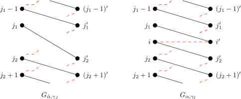
Figure 1. Adding a fixed point $i$ to a permutation $\tilde{\alpha}$ does not increase the number of cycles of $\tilde{\alpha}^{-1}\gamma_{J}$. Edges corresponding to $\alpha$ and $\tilde{\alpha}$ are represented by dashed red lines and edges corresponding to full cycles are black and solid.

2.2. A moment formula for the centered Wishart matrix

Let $G\in M_{d\times s}(\mathbf{C})$ be a Ginibre random matrix (i.e. $\{G_{ij}\}$ are i.i.d. standard complex Gaussian random variables) and $W=W_{d}=GG^{*}$ be the corresponding Wishart matrix of parameters $(d,s)$, where $G^{*}$ denotes the Hermitian adjoint of $G$. Here we make an abuse of notation and keep track only of the parameter $d$, considering implicitly that $s$ will be a function of $d$. It is easy to see that $\mathbb{E}W_{ij}=s\delta_{ij}$ and $\mathbb{E}\mathrm{tr}W=ds$.

The main theorem of this section characterizes the fluctuations of $W$ around its mean. For this purpose, we introduce the following $d\times d$ matrix, a properly rescaled, centered Wishart matrix of parameters $(d,s)$:

$$Z_{d}=\sqrt{ds}\left(\frac{W_{d}}{ds}-\frac{\mathbb{Id}_{d}}{d}\right),$$

where $\mathbb{Id}_{d}$ refers to the $d\times d$ identity matrix. We show that the following theorem holds true.

Theorem 2.2.

The moments of $Z_{d}$ are given by

(1) $$\mathbb{E}\frac{1}{d}\mathrm{tr}\left[Z_{d}\right]^{p}=\!\!\!\!\!\sum_{\alpha\in S^{o}_{p}}d^{-2g(\alpha)}\left(\frac{d}{s}\right)^{|\alpha|-p/2}.$$

Note that despite the simplicity of this combinatorial result, it seems to be new. Before we prove this result, we would like to describe three corollaries, obtained by letting one or both parameters $d$ and $s$ go to infinity.

Corollary 2.3.

If $d$ is fixed and $s\to\infty$, then

$$\lim_{s\to\infty}\mathbb{E}\frac{1}{d}\mathrm{tr}\left[Z_{d}\right]^{p}=\begin{cases}0,&\qquad\text{if $p$ is odd},\\ \sum_{g=0}^{\infty}\varepsilon(p/2,g)d^{-2g},&\qquad\text{if $p$ is even},\\ \end{cases}$$

where $\varepsilon(p/2,g)$ is the number of products of $p/2$ disjoint transpositions in $\mathcal{S}_{p}$ of genus $g$. Alternatively, for even $p$, $\varepsilon(p/2,g)$ is known to count the number of gluings of a $p$-gon into a surface of genus $g$.

Proof.

When $s\to\infty$, $d/s\to 0$ the only terms in equation (1) which survive are those for which $|\alpha|=p/2$. It follows that $\alpha$ must be in this case a product of $p/2$ disjoint transpositions (for even $p$). Reordering the sum by genera gives the statement (see [43]). ∎

Note that the sequence $\varepsilon(p,g)$ appears in the Online Encyclopedia of Integer Sequences [29] as A035309.

For the forthcoming corollary, we need to recall that the set $NC(p)$ is the collection of partitions of $[p]$ that have no crossings with respect to the canonical order. Moreover, we introduce the subset

$$NC^{o}(p)=\{\pi\in NC(p)\,|\,\pi\text{ has no singletons}\}.$$

Corollary 2.4.

If both $d,s\to\infty$ such that $s/d\to c$ for some constant $c>0$, we obtain

$$\lim_{\begin{subarray}{c}d,s\to\infty\\ s/d\to c\end{subarray}}\mathbb{E}\frac{1}{d}\mathrm{tr}\left[Z_{d}\right]^{p}=\sum_{\pi\in NC^{o}(p)}c^{\#\pi-p/2},$$

where $\#\pi$ denotes the number of blocks of the partition $\pi$. In particular, the random matrix $Z_{d}$ converges in moments to a centered Marchenko-Pastur distribution of parameter $c$ (rescaled by $\sqrt{c}$).

Proof.

In this asymptotic regime, the surviving terms in equation (1) are those for which $g(\alpha)=0$. The formula in the statement follows from a well known result of Biane [8] saying that the permutations in $\mathcal{S}_{p}$ of genus $0$ are in one to one correspondence with non-crossing partitions $\pi\in NC(p)$. The second part follows from a centered version of the free Poisson limit theorem [26, Theorem 12.11]. For $c=1$, the rescaled quantities appearing in the statement are the Riordan numbers $R_{p}$ [29, sequence A005043 ] such that $R_{p}=|NC^{o}(p)|$; see [28] for the connection between Riordan numbers and centered free Poisson random variables. ∎

Finally, we have the following general asymptotics

Corollary 2.5.

If $d\to\infty$ and $s/d\to\infty$ (in other words $1\ll d\ll s$), then

$$\lim_{\begin{subarray}{c}d\to\infty\\ s/d\to\infty\end{subarray}}\mathbb{E}\frac{1}{d}\mathrm{tr}\left[Z_{d}\right]^{p}=\begin{cases}0,&\qquad\text{if $p$ is odd},\\ \mathrm{Cat}_{p/2},&\qquad\text{if $p$ is even},\\ \end{cases}$$

where $\mathrm{Cat}_{n}$ is the $n$-th Catalan number. In particular, the random matrix $Z_{d}$ converges in moments to a standard semicircular distribution.

Proof.

This follows directly from the fact that the Catalan numbers count the number of non-crossing pairings of $[2p]$: $\varepsilon(2p,0)=\mathrm{Cat}_{p}$. ∎

Note that the above result also follows from the more general result by [7], where the almost sure convergence is also obtained. A proof of the almost sure convergence could also be obtained in the combinatorial spirit of this paper, for instance along the lines of [12].

We would like to explain briefly why this result is not surprising from a heuristic point of view. Indeed, the distribution for Marcenko-Pastur distribution, as given in Proposition 4.3, is

$$\pi_{c}=\frac{\sqrt{4c-(x-1-c)^{2}}}{2\pi x}\mathbf{1}_{[(\sqrt{c}-1)^{2},(\sqrt{c}+1)^{2}]}(x)\,dx,$$

so as $c\to\infty$, the distribution of $Z_{d}$ should approach

$$\sqrt{s/d}\frac{\sqrt{(2+\sqrt{d/s}-x)(x-2+\sqrt{d/s})}}{2\pi(x+\sqrt{s/d})}\mathbf{1}_{[-2+\sqrt{d/s},2+\sqrt{d/s}]}(x)\,dx$$

which should tend to the semi circle distribution. Our corollary therefore implies that we let $d,s/d$ go to infinity separately or together with any correlation we like.

Let us now prove the combinatorial result.

Proof of Theorem 2.2..

The starting point is a formula for the moments of $W$, obtained via the Wick calculus (for an intuitive graphical approach to this problem, see [12]):

$$\mathbb{E}\mathrm{tr}(W^{p})=\sum_{\alpha\in\mathcal{S}_{p}}d^{\#(\alpha^{-1}\gamma)}s^{\#\alpha}=(ds)^{p}\sum_{\alpha\in\mathcal{S}_{p}}d^{-|\alpha^{-1}\gamma|}s^{-|\alpha|},$$

where $\gamma\in\mathcal{S}_{p}$ is the forward cycle $\gamma=(1\,2\,\cdots\,p)$. By applying the binomial formula for the commuting matrices $W$ and $\mathbb{Id}_{d}$, we get

$$m_{p} :=\mathbb{E}\frac{1}{d}\mathrm{tr}\left[\sqrt{ds}\left(\frac{W}{ds}-\frac{\mathbb{Id}_{d}}{d}\right)\right]^{p}$$

$$=d^{-1+p/2}s^{p/2}\sum_{I\subset[p]}(-1)^{|I^{c}|}(ds)^{|I|}d^{-|I^{c}|}\mathbb{E}\mathrm{tr}(W^{|I|})$$

$$=\sum_{I\subset[p]}\sum_{\alpha\in\mathcal{S}_{I}}(-1)^{p-|I|}d^{-1-p/2+|I|-|\alpha^{-1}\gamma|}s^{p/2-|\alpha|}$$

$$=\sum_{I\subset[p]}\sum_{\alpha\in\mathcal{S}_{I}}(-1)^{p-|I|}d^{-2g_{I}(\alpha)}\left(\frac{d}{s}\right)^{|\alpha|-p/2}.$$

To conclude, we need to show that the terms in the sum above cancel out, except for the ones with $I=[p]$ and $\alpha\in\mathcal{S}_{[p]}$ without fixed points. For a permutation $\tilde{\alpha}\in\mathcal{S}^{o}_{J}$, denote by $[\tilde{\alpha}]$ the set of permutations which extend $\tilde{\alpha}$ by adding fixed points:

$$[\tilde{\alpha}]=\{\alpha\in\mathcal{S}_{I}\,|\,J\subset I\text{ , }\alpha(j)=\tilde{\alpha}(j)\quad\forall j\in J\text{ and }\alpha(i)=i\quad\forall i\in I\setminus J\}.$$

Regrouping terms in the sum and using the fact that for $\alpha\in[\tilde{\alpha}]$, $|\alpha|=|\tilde{\alpha}|$ and $g_{I}(\alpha)=g_{J}(\tilde{\alpha})$, we can write

$$m_{p}=\sum_{\tilde{\alpha}\in\mathcal{S}^{o}}d^{-2g_{J}(\tilde{\alpha})}\left(\frac{d}{s}\right)^{|\tilde{\alpha}|-p/2}\sum_{\alpha\in\mathcal{S}_{I}\cap[\tilde{\alpha}]}(-1)^{p-|I|},$$

where the first sum in the equation above is indexed by permutations $\tilde{\alpha}$ without fixed points. Given such a permutation $\tilde{\alpha}\in\mathcal{S}_{J}$, for every larger set $I\supset J$ there is a unique way of extending $\tilde{\alpha}$ to $\alpha\in\mathcal{S}_{I}$. Hence, the second sum in the above equation is given by

$$\sum_{J\subset I\subset[p]}(-1)^{p-|I|}=\delta_{J,[p]},$$

which can be understood as a Möbius inversion formula in the poset of subsets of $[p]$. In conclusion, only the permutations $\tilde{\alpha}\in\mathcal{S}^{o}_{p}$ give non-zero contribution. To finalize the proof, note that such a permutation has at most $p/2$ cycles and thus at least length $p/2$. ∎

2.3. Almost sure convergence of extremal eigenvalues of the Wishart matrices in the regime $d\ll s$

We start with the following lemma:

Lemma 2.6.

Let us assume that $d/s\to c\in(0,\infty)$ as $d\to\infty$. For any $\varepsilon>0$ there exists a constant $C>0$ such that for any $p\leqslant\sqrt{d}$, we have

$$\operatorname{\mathbb{E}}\mathrm{tr}Z_{d}^{p}\leqslant C(2+\sqrt{c}+\varepsilon)^{p}.$$

Proof.

Under the hypotheses of the lemma, the eigenvalues counting measure of $Z_{d}$ converges almost surely to a probability measure whose support is $[-2+\sqrt{c},2+\sqrt{c}]$.

Let us first evaluate $\mathbb{P}(\|Z_{d}\|\geqslant 2+\sqrt{c})$, where $\|Z_{d}\|$ is the operator norm of $Z_{d}$. According to the union bound, this is bounded above by

$$\mathbb{P}(\lambda_{1}(Z_{d})\geqslant 2+\sqrt{c})+\mathbb{P}(\lambda_{d}(Z_{d})\leqslant-2-\sqrt{c}),$$

where $\lambda_{1}(Z_{d})$ and $\lambda_{d}(Z_{d})$ are respectively the largest and smallest eigenvalues of $Z_{d}$.

According to Theorem 3 of Soshnikov in [33], there exists a constant $C>0$ such that for any $p\leqslant\sqrt{d}$, we have

$$\operatorname{\mathbb{E}}\mathrm{tr}W_{d}^{p}\leqslant C(\sqrt{c}+1)^{2p}.$$

By Jensen inequality this implies under the same assumption on $p$ that

$$\mathbb{P}(\lambda_{1}\geqslant(\sqrt{c}+1)^{2}+t)\leqslant\frac{(\sqrt{c}+1)^{2p}}{[(\sqrt{c}+1)^{2}+t]^{p}}.$$

Besides, it follows from Equation (15) in [24], that the probability of having eigenvalues less than $t<(\sqrt{c}-1)^{2}$ is less than $\exp(-dg(t))$. For our purposes it is enough to know that $g(t)>0$ as long as $0<t<(\sqrt{c}-1)^{2}$.

We can conclude the proof of the lemma from the two above observations via the inequalities

$$\lambda_{1}^{p}\leqslant\mathrm{tr}W^{p}\leqslant n\lambda_{1}^{p},$$

and the formula

$$\operatorname{\mathbb{E}}(X)=\int_{0}^{\infty}\mathbb{P}(X\geqslant t)dt.$$

∎

Now we would like to let $s/d\to\infty$ simultaneously (but independently) with $d\to\infty$. This is the setting of our next result, namely:

Theorem 2.7.

Almost surely, when $1\ll d\ll s$, the extremal eigenvalues of $Z_{d}$ converge to $\pm 2$.

Proof.

Let $\varepsilon>0$ and $d_{0}$ large enough such that for $d\geqslant d_{0}$, $\sqrt{d/s}\leqslant\varepsilon/2$. The moment inequality from Lemma 2.6 together with the fact that our moment formula of Theorem 2.2 involves only positive terms implies that there exists a constant $C>0$, such that for all $p\leqslant\sqrt{d}$,

$$\operatorname{\mathbb{E}}(\mathrm{tr}Z_{d}^{p})\leqslant C(2+\varepsilon)^{p}.$$

Letting $d\to\infty$, by the Borel-Cantelli Lemma and the same Jensen inequality as in the proof of Lemma 2.6, we obtain that $\limsup\lambda_{1}\leqslant 2+\varepsilon$ almost surely. Since this holds true for all $\varepsilon>0$ and since $\liminf\lambda_{1}\geqslant 2$ by Corollary 2.5, we get the desired result. ∎

An interesting aspect of the above proof is that it relies on moment techniques, and therefore makes use of Theorem 2.2. Here the interest of the moment method and combinatorics is that they explain why one can make rigorous a change of limit between $d\to\infty$ and $s/d\to\infty$ regarding the almost sure convergence of the largest eigenvalue.

We could have obtained directly this result with complex analysis results (see e.g. [9]) and one could probably have obtained more refined estimates (e.g. large deviation bounds, universality results, etc); however, this was not in the spirit of our combinatorial approach and we leave it for future investigation.

Using similar techniques, one could extend the above results to show the following quantitative bound: for all $\varepsilon>0$, with exponential small probability in $d\to\infty$, the spectrum of a random density matrix $\rho$ from the induced ensemble of parameters $(d,s)$ is contained in the interval

$$\left[\frac{1}{d}-\frac{2(1+\varepsilon)}{\sqrt{ds}},\frac{1}{d}+\frac{2(1+\varepsilon)}{\sqrt{ds}}\right].$$

3. Existence of a threshold for $\mathcal{APPT}$

3.1. Quantum states and Absolute PPT

We now introduce some necessary notation and concepts related to quantum information theory; readers are referred to [11] and [27] for more details.

Consider a (complex) Hilbert space $\mathbf{C}^{d}=\mathbf{C}^{d_{1}}\otimes\cdots\otimes\mathbf{C}^{d_{k}}$ with (complex) dimension $d=d_{1}\cdots d_{k}$, where $d_{i}\geqslant 2$ for all $i=1,\cdots,k$. The set of states on $\mathbf{C}^{d}$ (denoted by $\mathcal{D}=\mathcal{D}(\mathbf{C}^{d})$) can be identified with the set of $d\times d$ density matrices. That is,

$$\mathcal{D}=\{\rho\in M^{\text{sa}}_{d}(\mathbf{C})\,|\,\rho\geqslant 0\text{ and }\mathrm{tr}\rho=1\}.$$

Clearly the real dimension of $\mathcal{D}$ is $N=d^{2}-1$. The set $\mathcal{D}$ is contained in the affine hyperplane

$$H_{1}=\{A\in M^{\text{sa}}_{d}(\mathbf{C})\,|\,\mathrm{tr}A=1\},$$

endowed with the Hilbert-Schmidt inner product $\langle A,B\rangle=\operatorname{\mathrm{tr}}(A^{*}B)$.

Partial tracing states on $\mathbf{C}^{d}\otimes\mathbf{C}^{s}$ over $\mathbf{C}^{s}$ gives reduced density matrices of size $d\times d$. Any state $\rho$ on $\mathbf{C}^{d}\otimes\mathbf{C}^{s}$ may be written as

$$\rho=\sum_{i,j}^{d}\sum_{\alpha,\beta}^{s}\rho_{i\alpha,j\beta}E_{i\alpha,j\beta},$$

where $E_{i\alpha,j\beta}$ are the matrix units associated to orthonormal bases $\{e_{i}\}_{i=1}^{d}$ and $\{f_{\alpha}\}_{\alpha=1}^{s}$ of $\mathbf{C}^{d}$ and $\mathbf{C}^{s}$ respectively. The partial trace of $\rho$ over $\mathbf{C}^{s}$, denoted by $\sigma=\mathrm{tr}_{\mathbf{C}^{s}}(\rho)$ may be formulated as

$$\sigma_{ij}=\sum_{\beta=1}^{s}\rho_{i\beta,j\beta}\ \mathrm{for}\ i,j=1,\cdots,d.$$

The induced measure on $\mathcal{D}(\mathbf{C}^{d})$ by partial tracing over $\mathbf{C}^{s}$ is an important probability distribution and can be described as follows. Let $|\psi\rangle\langle\psi|$ be a random pure state on $\mathbf{C}^{d}\otimes\mathbf{C}^{s}$, where $\psi$ is a random unit vector uniformly distributed on the sphere in $\mathbf{C}^{d}\otimes\mathbf{C}^{s}$. Then the random induced state $\rho=\mathrm{tr}_{\mathbf{C}^{s}}(|\psi\rangle\langle\psi|)\in\mathcal{D}(\mathbf{C}^{d})$ follows the distribution $\mu_{d,s}$. Equivalently, one can find a $d\times s$ matrix $M$ distributed uniformly on the sphere of $d\times s$ matrices, such that $\rho=MM^{*}.$ The distribution $\mu_{d,s}$ plays central roles in this section. When $s=d$, one gets $\mu_{d,d}$, the normalized Lebesgue (i.e., the Hilbert-Schmidt) measure on $\mathcal{D}(\mathbf{C}^{d})$. Hence, a random state distributed according to $\mu_{d,d}$ is uniformly distributed on $\mathcal{D}(\mathbf{C}^{d})$. When $s\geqslant d$, the probability measure $\mu_{d,s}$ has a simple form [44]

(2) $$\frac{d\mu_{d,s}}{d\!\operatorname{\mathrm{vol}}}(\rho)=\frac{1}{Z_{d,s}}(\det\rho)^{s-d},$$

where $Z_{d,s}$ is a normalization factor. Note that formula (2) allows to define the measure $\mu_{d,s}$ (in particular) for every real $s\geqslant d$, while the partial trace construction makes sense only for integer values of $s$.

Hereafter, we will focus on the bipartite system, i.e, the case $\mathbf{C}^{d}=\mathbf{C}^{d_{1}}\otimes\mathbf{C}^{d_{2}}$ with $d=d_{1}d_{2}$. The partial transpose operator (denoted by $T_{2}$) is a linear operation that consists in taking the transpose in one leg and doing nothing on the other leg, i.e., $T_{2}(\tau_{1}\otimes\tau_{2})=\tau_{1}\otimes\tau_{2}^{T}$, where $T$ is the normal transpose operator. The set of quantum states with positive partial transpose is denoted by $\mathcal{PPT}$, i.e., $\rho\in\mathcal{PPT}$ if and only if $T_{2}(\rho)\geqslant 0$. Geometrically, $\mathcal{PPT}=\mathcal{D}\cap T_{2}(\mathcal{D})$, and $\mathcal{PPT}$ is a convex body with constant height [36]. Peres-Horodecki PPT criterion states that $\mathcal{S}\subset\mathcal{PPT}$ [22, 30], and $\mathcal{S}=\mathcal{PPT}$ only if $d\leqslant 6$ [34, 40]. Here, the $N=d^{2}-1$ dimensional set $\mathcal{S}\subset\mathcal{D}$ is the set of separable quantum states on $\mathbf{C}^{d}$ [39] defined as

$$\mathcal{S}=\mathcal{S}(\mathbf{C}^{d_{1}}\otimes\mathbf{C}^{d_{2}}):={\rm conv}\{\rho_{1}\otimes\rho_{2},\ \ \rho_{1}\in\mathcal{D}(\mathbf{C}^{d_{1}}),\ \ \rho_{2}\in\mathcal{D}(\mathbf{C}^{d_{2}})\}.$$

(Similarly, one can define $\mathcal{S}(\mathbf{C}^{d_{1}}\otimes\cdots\otimes\mathbf{C}^{d_{k}})$.) The set $\mathcal{E}:=\mathcal{D}\setminus\mathcal{S}$ is the set of entangled quantum states, which play a crucial role in quantum information and quantum computing.

A quantum state $\rho\in\mathcal{D}(\mathbf{C}^{d_{1}}\otimes\mathbf{C}^{d_{2}})$ is absolutely PPT(or APPT) if for any unitary matrix $U\in\mathcal{U}(d)$, $U\rho U^{*}\in\mathcal{PPT}$. The set of all states being APPT, denoted as $\mathcal{APPT}$, is

(3) $$\mathcal{APPT}=\bigcap_{U\in\mathcal{U}(d)}U(\mathcal{PPT})U^{*}\subset\mathcal{PPT}.$$

Clearly, $\mathcal{APPT}$ is a convex body, a convex compact set with non-empty interior. This follows easily from (3) and the following result in [17]: $\epsilon\mathcal{D}+(1-\epsilon)\frac{\mathbb{I}}{d}\subset\mathcal{S}\subset\mathcal{PPT}$ for some $\epsilon<\frac{1}{d-1}$.

In applications, one often requires the convex bodies to be origin-symmetric. In this section, we will mainly work on the symmetric convex body $\mathcal{APPT}_{\textnormal{sym}}=-\mathcal{APPT}_{0}\cap\mathcal{APPT}_{0}$ where $\mathcal{APPT}_{0}=\mathcal{APPT}-\mathbb{I}/d$. Such a symmetrization will not change many geometric parameters of interest (such as, the volume radius and mean width) substantially, due to the famous Rogers-Shephard inequality [31]. Both $\mathcal{APPT}_{0}$ and $\mathcal{APPT}_{\textnormal{sym}}$ sit in the linear hyperplane

$$H_{0}=\{A\in M^{\text{sa}}_{d}(\mathbf{C})\,|\,\mathrm{tr}A=0\}.$$

Recall that the gauge associated to a convex body $K\subset\mathbf{R}^{N}$ is the function $\|\cdot\|_{K}$ defined by

$$\|x\|_{K}=\inf\{t\geqslant 0\ :\ x\in tK\},\ \ \ \forall x\in\mathbf{R}^{N}.$$

Note that $\|x\|_{K}=\|-x\|_{K}$ for origin-symmetric convex bodies $K$. The outradius of $K$ is the smallest $R>0$ such that $K$ is contained in a ball of radius $R$. Similarly, the inradius of a convex body $K$ is the largest radius $r$ of a Euclidean ball contained in $K$. For origin-symmetric convex bodies, $r$ and $R$ can be defined as the “best” constants such that $R^{-1}|\cdot|\leqslant\|\cdot\|_{K}\leqslant r^{-1}|\cdot|$ (where $|\cdot|$ denotes the Euclidean norm.) Let $X$ be a standard Gaussian vector in $\mathbf{R}^{N}$, i.e., a random vector with independent $N(0,1)$ coordinates in any orthonormal basis.

Proposition 3.1.

In the notation of the present section, we have

(4) $$d^{1/2}|\cdot|\leqslant\|\cdot\|_{\mathcal{APPT}_{\textnormal{sym}}}\leqslant d|\cdot|\iff d^{-1}|\cdot|\leqslant\|\cdot\|_{\mathcal{APPT}_{\textnormal{sym}}^{\circ}}\leqslant d^{-1/2}|\cdot|,$$

(5) $$\operatorname{\mathbb{E}}\|X\|_{\mathcal{APPT}_{0}}\leqslant\operatorname{\mathbb{E}}\|X\|_{\mathcal{APPT}_{\textnormal{sym}}}\leqslant 2\operatorname{\mathbb{E}}\|X\|_{\mathcal{APPT}_{0}}.$$

Proof.

Any matrix $A\in\mathcal{APPT}_{0}$ satisfies $A\geqslant-\mathbb{Id}/d$. This implies that any $A\in\mathcal{APPT}_{\textnormal{sym}}$ satisfies $-\mathbb{Id}/d\leqslant A\leqslant\mathbb{Id}/d$, or $\|A\|_{\infty}\leqslant 1/d$, and therefore the outradius of $\mathcal{APPT}_{\textnormal{sym}}$ is bounded by $1/\sqrt{d}$. The inradius of $\mathcal{APPT}$ equal to $(d(d-1))^{-1/2}$ follows directly from Corollary 3 in [17]. This proves (4).

Note that the distribution of $X$ is symmetric, and

$$\|X\|_{\mathcal{APPT}_{0}} \leqslant\|X\|_{\mathcal{APPT}_{\textnormal{sym}}}$$

$$=\max(\|X\|_{\mathcal{APPT}_{0}},\|-X\|_{\mathcal{APPT}_{0}})\leqslant\|X\|_{\mathcal{APPT}_{0}}+\|-X\|_{\mathcal{APPT}_{0}}.$$

Then (5) follows after taking expectation. ∎

It was pointed out that the set $\mathcal{APPT}$ varies if the decomposition of $d$ changes: if $\min(d_{1}^{\prime},d_{2}^{\prime})\geqslant\min(d_{1},d_{2})$, then any APPT quantum states on $\mathbf{C}^{d_{1}^{\prime}}\otimes\mathbf{C}^{d_{2}^{\prime}}$ must be APPT on $\mathbf{C}^{d_{1}}\otimes\mathbf{C}^{d_{2}}$ [20]. Consequently, the largest APPT set is obtained when $d_{1}=2$ and $d_{2}=d/2$, and the smallest APPT set is obtained when $d_{1}=d_{2}=\sqrt{d}$.

Let $p=\min(d_{1},d_{2})$. Denote by $S_{+}=\{(k,l):1\leqslant k\leqslant l\leqslant p\}$ and $S_{-}=\{(k,l):1\leqslant k<l\leqslant p\}$. Note that the cardinalities of the sets $S_{+}$ and $S_{-}$ are $p_{+}=p(p+1)/2$ and $p_{-}=p(p-1)/2$ respectively. Let

$$\sigma_{+}:S_{+}\rightarrow\{1,\cdots,p_{+}\},\ \ \mathrm{and}\ \ \sigma_{-}:S_{-}\rightarrow\{1,\cdots,p_{-}\},$$

be two orderings (i.e. bijective maps) on $S_{+}$ and $S_{-}$ respectively. Thus, $\sigma_{+}(k,l)\leqslant p_{+}$ and $\sigma_{-}(k,l)\leqslant p_{-}$ for all pairs $(k,l)$.

For $\lambda=(\lambda_{1},\cdots,\lambda_{d})$ with ordering $\lambda_{1}\geqslant\lambda_{2}\geqslant\cdots\geqslant\lambda_{d}\geqslant 0$ and $\sum_{i=1}^{d}\lambda_{i}=1$, one defines the matrix $\Lambda(\lambda;\sigma_{+},\sigma_{-})$ as

$$\big{(}\Lambda(\lambda;\sigma_{+},\sigma_{-})\big{)}_{k,l}=\left\{\begin{array}[]{cc}\lambda_{d+1-\sigma_{+}(k,l)},&k\leqslant l;\\ -\lambda_{\sigma_{-}{(l,k)}},&k>l.\end{array}\right.$$

Define the $p\times p$ symmetric matrix $\Theta(\lambda;\sigma_{+},\sigma_{-})$ to be the sum of $\Lambda(\lambda;\sigma_{+},\sigma_{-})$ and its transpose $\Lambda^{T}(\lambda;\sigma_{+},\sigma_{-}).$ Note that $\Theta(\lambda;\sigma_{+},\sigma_{-})$ has the following form:

(6) $$\Theta_{k,l}=\left\{\begin{array}[]{cc}2\lambda_{a(k)},&k=l,\\ \lambda_{b(k,l)}-\lambda_{c(k,l)},&b(k,l)>c(k,l),k>l,\end{array}\right.$$

where $a(k)$, $b(k,l)$ and $c(k,l)$ are some integer-valued functions with values smaller than or equal to $d$. Thus $\Theta_{k,l}\leqslant 0$ for all $k\neq l$.

The following theorem is a necessary and sufficient condition for $\rho\in\mathcal{APPT}$ (see Theorem III.9 or Lemma III.10 in [20] ).

Theorem 3.2.

Let $\rho$ be a quantum state on $\mathbf{C}^{d}=\mathbf{C}^{d_{1}}\otimes\mathbf{C}^{d_{2}}$ with $d=d_{1}d_{2}$. Suppose that $\rho$ has eigenvalues $\lambda_{1}\geqslant\lambda_{2}\geqslant\cdots\geqslant\lambda_{d}\geqslant 0$. Then $\rho$ is $\mathcal{APPT}$ if and only if for all pair of ordering $(\sigma_{+},\sigma_{-})$, $\Theta(\lambda;\sigma_{+},\sigma_{-})$ is positive semi-definite.

3.2. Threshold for $\mathcal{APPT}$ is $\sim w(\mathcal{APPT}_{0}^{\circ})^{2}$.

Hereafter, $w(\mathcal{APPT}_{0}^{\circ})$ denotes the mean width of $\mathcal{APPT}_{0}^{\circ}$, the polar body of $\mathcal{APPT}_{0}$. For general convex body $K$ with the origin in its interior, its polar body (denoted by $K^{\circ}$) can be defined as

$$K^{\circ}=\{y\in\mathbf{R}^{N}\ :\ \langle x,y\rangle\leqslant 1\ \ \forall x\in K\},$$

where $\langle\cdot,\cdot\rangle$ denotes the usual inner product and induces the Euclidean norm $|\cdot|$. The mean width of $K$, $w(K)$, is defined as

(7) $$w(K):=\int_{S^{N-1}}h_{K}(u)\,d\sigma(u)=\int_{S^{N-1}}\|u\|_{K^{\circ}}d\sigma(u),$$

where $\,d\sigma(u)$ is the normalized spherical measure on the sphere $S^{N-1}$, and $h_{K}(u)=\max_{x\in K}\langle x,u\rangle=\|u\|_{K^{\circ}}$ for any $u\in S^{N-1}$. A more convenient quantity to calculate is the Gaussian mean width of $K$

(8) $$w_{G}(K)=\operatorname{\mathbb{E}}\|X\|_{K^{\circ}}=\operatorname{\mathbb{E}}\sup_{x\in K}\langle X,x\rangle,$$

where $X$ is a standard Gaussian vector in $\mathbf{R}^{N}$. By passing to polar coordinates, one can easily check that for every convex body $K\subset\mathbf{R}^{N}$

(9) $$w_{G}(K)=\gamma_{N}\,w(K),$$

where

(10) $$\gamma_{N}=\operatorname{\mathbb{E}}|G|=\frac{\sqrt{2}\Gamma((N+1)/2)}{\Gamma(N/2)},\quad\sqrt{N-1}\leqslant\gamma_{N}\leqslant\sqrt{N},$$

is a constant depending only on $N$. We set $s_{0}(d_{1},d_{2})$ to be

$$s_{0}=s_{0}(d_{1},d_{2})=\left(\frac{\operatorname{\mathbb{E}}\|X\|_{\mathcal{APPT}_{0}}}{d^{2}}\right)^{2}=\left(\frac{w_{G}(\mathcal{APPT}_{0}^{\circ})}{d^{2}}\right)^{2}\sim w(\mathcal{APPT}_{0}^{\circ})^{2}.$$

By inequality (5), one has $s_{0}\sim w(\mathcal{APPT}_{0}^{\circ})^{2}\simeq w(\mathcal{APPT}_{\textnormal{sym}}^{\circ})^{2}$. The following theorem states that the threshold for the set $\mathcal{APPT}$ is of order of $w(\mathcal{APPT}_{0}^{\circ})^{2}$.

Theorem 3.3.

There are effectively computable absolute constants $C,c>0$, such that, if $\rho$ is a random induced state on $\mathbf{C}^{d_{1}}\otimes\mathbf{C}^{d_{2}}$ distributed according to the measure $\mu_{d,s}$, then

• $\mathbb{P}(\rho\in\mathcal{APPT})\leqslant C\exp(-cs)$ for $s\leqslant cs_{0}$;

• $\mathbb{P}(\rho\notin\mathcal{APPT})\leqslant C\exp(-cs_{0})$ for $s\geqslant Cs_{0}$.

We first point out that the threshold value for the set $\mathcal{PPT}$ occurs only at those $s\geqslant 2d$. For the balanced bipartite case (i.e. $d_{1}=d_{2}$) it follows from Theorem 4 in [1], while for the unbalanced bipartite case (i.e., $d_{1}\neq d_{2}$) it follows from [10]. As $\mathcal{APPT}\subset\mathcal{PPT}$, the threshold for $\mathcal{APPT}$ must be larger and thus we also have $s\geqslant 2d$.

The following lemma is our main tool to prove that the threshold for the set $\mathcal{APPT}$ can be taken as $w(\mathcal{APPT}_{0}^{\circ})^{2}$. This lemma aims to approximate $\rho-\mathbb{Id}/d$ by $\frac{1}{d\sqrt{s}}X$ where $X$ is a standard Gaussian vector in the space $H_{0}$ of traceless Hermitian $d\times d$ matrices. We refer readers to its detailed proof in [4].

Lemma 3.4.

For every convex body $K\subset H_{0}$ containing $0$ in its interior, and for every $s\geqslant d$, if $\rho$ is a random state on $\mathbf{C}^{d}$ distributed according to $\mu_{d,s}$, and if $X$ is a standard Gaussian vector in $H_{0}$, then

$$\operatorname{\mathbb{E}}\left\|\rho-\frac{\mathbb{Id}}{d}\right\|_{K}\simeq\frac{1}{d\sqrt{s}}\operatorname{\mathbb{E}}\|X\|_{K}.$$

Applying the lemma for $K=\mathcal{APPT}_{0}$, we obtain that

(11) $$\operatorname{\mathbb{E}}\left\|\rho-\frac{\mathbb{Id}}{d}\right\|_{\mathcal{APPT}_{0}}\simeq\sqrt{\frac{s_{0}(d)}{s}}.$$

This suggests that the threshold for the set $\mathcal{APPT}_{0}$ occurs at $s_{0}(d)$, since a state $\rho$ is APPT when $\|\rho-\mathbb{Id}/d\|_{\mathcal{APPT}_{0}}\leqslant 1$ and non-APPT when $\|\rho-\mathbb{Id}/d\|_{\mathcal{APPT}_{0}}>1$.

The proof of Theorem 3.3 is almost identical to that of Section 4 in [4], and here we sketch its proof for completeness. We refer the readers to [4] for more details, in particular Appendix E for the Lévy’s Lemma and concentration of measure theory.

Proof of Theorem 3.3..

Let $S_{HS}$ be the Hilbert-Schmidt sphere in the space of $d\times s$ matrices (it can be identified with the real sphere $S^{2ds-1}$) and $f:S_{HS}\to\mathbf{R}$ be the function defined by

$$f(M)=\left\|MM^{*}-\frac{\mathbb{Id}}{d}\right\|_{\mathcal{APPT}_{0}}.$$

Formula (11) asserts that $\operatorname{\mathbb{E}}f\simeq\sqrt{\frac{s_{0}(d)}{s}}.$ For every $r>0$, denote by $\Omega=\Omega(r)$ the subset

$$\Omega=\{M\in S_{HS}\ :\ \|M\|_{\infty}\leqslant r\}.$$

Inequality (4) and the proof of Lemma 4.2 in [4] imply that the Lipschitz constant of $f|_{\Omega}$ is bounded by $2rd$. Note that $\Omega(r)=S_{HS}$ since $\|M\|_{\infty}\leqslant\|M\|_{2}=1$. Then, the global Lipschitz constant of $f$ is bounded by $2d$, and hence the median of $f$ (denoted $M_{f}$) differs from its mean, $\operatorname{\mathbb{E}}f$, by at most $C2d/\sqrt{2ds}=C^{\prime}\sqrt{d/s}$ (see Appendix E in [4]). It follows that the median of $f$ is also of order $\sqrt{s_{0}/s}$.

By a net argument similar to that in [3], one has $\mathbb{P}(S_{HS}\setminus\Omega)\lesssim\exp(-cs)$ if $r=3/\sqrt{d}$. A local version of Lévy’s lemma (see Appendix E in [4]) implies that for $\varepsilon=M_{f}/2\simeq\sqrt{s_{0}/s}$,

$$\mathbb{P}(|f-M_{f}|\geqslant M_{f}/2) =\mathbb{P}(|f-M_{f}|\geqslant\varepsilon)$$

$$\lesssim\mathbb{P}(S_{HS}\setminus\Omega)+\exp(-c_{1}ns(\varepsilon/2dr)^{2})$$

$$\lesssim\exp(-cs)+\exp(-cs_{0}).$$

Therefore, one has

$$\mathbb{P}(\rho\textnormal{ is APPT})=\mathbb{P}(f\leqslant 1)\lesssim\exp(-cs),$$

whenever $M_{f}\geqslant 2$ (or, equivalently, $s\lesssim s_{0}$) and

$$\mathbb{P}(\rho\textnormal{ is not APPT})=\mathbb{P}(f>1)\lesssim\exp(-cs_{0}),$$

whenever $M_{f}\leqslant 2/3$ (or, equivalently, $s\gtrsim s_{0}$). This ends the proof of Theorem 3.3. ∎

4. Estimates on the threshold for $\mathcal{APPT}$

We consider the product systems $\mathbf{C}^{d}=\mathbf{C}^{d_{1}}\otimes\mathbf{C}^{d_{2}}$. Recall that a random state $\rho$ on $\mathbf{C}^{d}=\mathbf{C}^{d_{1}}\otimes\mathbf{C}^{d_{2}}$ distributed according to $\mu_{d,s}$ has the same distribution as $MM^{*}$, where $M$ is a $d\times s$ matrix uniformly distributed on the Hilbert-Schmidt sphere of the Hilbert space of $d\times s$ complex matrices. A more convenient, but equivalent, way is to link the measure $\mu_{d,s}$ with a normalized Wishart matrix. More precisely, let $W=GG^{*}$, where $G\in M_{d\times s}(\mathbf{C})$ is a Ginibre matrix, i.e. a matrix with i.i.d. standard complex Gaussian entries. The random matrix $W$ is called a Wishart matrix of parameters $(d,s)$. A random induced state $\rho$ distributed according to $\mu_{d,s}$ is then given by the formula $\rho=W/\mathrm{tr}W$ [25, 44].

The following theorem is the main result of this section, providing asymptotic values of the threshold for the convex body $\mathcal{APPT}$. This theorem covers the case when $p=\min(d_{1},d_{2})\to\infty$. The simpler case of $p$ bounded is treated in Theorem 4.2 as it gives sharper bounds.

Theorem 4.1.

Let $\rho$ be a random induced state distributed according to the probability measure $\mu_{d,s}$.

• For all $\varepsilon>0$, almost surely, when $d\to\infty$ and $s>(4+\varepsilon)p^{2}d$, the quantum state $\rho$ is APPT;

• When $1\ll p^{2}\ll d$ and $s<(4-\varepsilon)p^{2}d$, $\rho$ is not APPT almost surely;

• When $p^{2}\sim\tau d$ for a constant $\tau\in(0,1]$, there exists a constant $C_{\tau}$ (see formula (13)) such that whenever and $s<4(C_{\tau}-\varepsilon)p^{2}d$, $\rho$ is not APPT almost surely.

Proof.

We start with (i). For given eigenvalues $\{\lambda_{1},\cdots,\lambda_{d}\}$, we introduce the following $p\times p$ matrix:

$$\Upsilon=\Upsilon(\lambda;\sigma_{+},\sigma_{-})=\Theta(\lambda;\sigma_{+},\sigma_{-})-2d^{-1}\mathbb{Id}_{p},$$

where $\mathbb{Id}_{p}$ denotes the $p\times p$ identity matrix. Recall that $p=\min(d_{1},d_{2})$. From formula (6) and Theorem 2.7, the matrix $\Upsilon$ has small entries: $|\Upsilon_{ij}|\leqslant(4+\varepsilon)/\sqrt{ds}$. A necessary condition for the matrix $\Theta=2d^{-1}\mathbb{Id}_{p}+\Upsilon$ to be semidefinite positive is that $\Upsilon$ should have operator norm smaller than $2/d$. It is a well known fact in matrix analysis (see [21]) that

$$\|\Upsilon\|_{\text{op}}\leqslant p\|\Upsilon\|_{1\to\infty}=p\max_{1\leqslant i,j\leqslant p}|\Upsilon_{ij}|\leqslant\frac{(4+\varepsilon)p}{\sqrt{ds}}.$$

The conclusion in the statement follows by asking that $(4+\varepsilon)p/{\sqrt{ds}}\leqslant 2/d$.

We move now to the proofs of (ii) and (iii). We shall proceed by exhibiting a vector $x\in\mathbf{R}^{p}$, such that, $x^{T}\Lambda(\lambda;\sigma_{+},\sigma_{-})x<0$ for some pair of linear orderings. This does indeed suffice to show that the matrix $\Theta$ is not semidefinite positive. Indeed, we take the column vector $x=(1,1,\ldots,1)^{T}\in\mathbf{R}^{p}$. Any pair of linear orderings is compatible with such a vector, and one has

(12) $$x^{\prime}\Lambda(\lambda;\sigma_{+},\sigma_{-})x=\sum_{i,j=1}^{p}\Lambda_{ij}=\sum_{i=1}^{p_{+}}\lambda_{d+1-i}-\sum_{i=1}^{p_{-}}\lambda_{i},$$

where $p_{+}=p(p+1)/2$ and $p_{-}=p(p-1)/2$.

We shall now consider the two regimes in the statement, starting with $1\ll p^{2}\ll d$. The main idea here is to note that, for all $i$, $\lambda_{i}=1/d+\tilde{\lambda}_{i}/\sqrt{ds}$, where $\tilde{\lambda}_{i}$ are the eigenvalues of the matrix $Z_{d}$ introduced in Section 2.2. By Theorem 2.7, for all $\varepsilon>0$ and for $d$ large enough, all the “large” eigenvalues $\lambda_{1},\ldots,\lambda_{p_{-}}$ appearing in equation (12) are bigger than $1/d+(2-\varepsilon)/\sqrt{ds}$; in the same vein, all the “small” eigenvalues $\lambda_{d+1-p_{+}},\ldots,\lambda_{d}$ are smaller than $1/d-(2-\varepsilon)/\sqrt{ds}$. We obtain

$$x^{\prime}\Lambda(\lambda;\sigma_{+},\sigma_{-})x\leqslant p_{+}\left(\frac{1}{d}-\frac{2-\varepsilon}{\sqrt{ds}}\right)-p_{-}\left(\frac{1}{d}+\frac{2-\varepsilon}{\sqrt{ds}}\right)=\frac{p}{d}-\frac{(2-\varepsilon)p^{2}}{\sqrt{ds}},$$

which is negative as long as $s<(4-\varepsilon)p^{2}d$. This concludes the proof for the first regime $1\ll p^{2}\ll d$.

We now move on the the second regime, where $p^{2}\sim\tau d$, for a fixed constant $\tau\in(0,1]$. Writing equation (12) in terms of the eigenvalues of $Z_{d}$, we obtain

$$x^{\prime}\Lambda(\lambda;\sigma_{+},\sigma_{-})x=\frac{p}{d}+\frac{1}{\sqrt{ds}}\left[\sum_{i=1}^{p_{+}}\tilde{\lambda}_{d+1-i}-\sum_{i=1}^{p_{-}}\tilde{\lambda}_{i}\right].$$

Using the fact that the asymptotic spectrum $\{\tilde{\lambda}_{i}\}$ of $Z_{d}$ is semicircular, we obtain the following bounds for $d$ large enough:

$$\frac{1}{d}\sum_{i=1}^{p_{+}}\tilde{\lambda}_{d+1-i}\lesssim\int_{-2}^{-c_{\tau/2}-\varepsilon}xw(x)\mathrm{d}x,\ \ \ \mathrm{and}\ \ \ \frac{1}{d}\sum_{i=1}^{p_{-}}\tilde{\lambda}_{i}\gtrsim\int_{c_{\tau/2}+\varepsilon}^{2}xw(x)\mathrm{d}x,$$

where

$$w(x)=\frac{1}{2\pi}\sqrt{4-x^{2}}$$

is the density of the standard semicircular distribution and $c_{\tau/2}\in[0,2]$ is defined implicitly by

$$\int_{c_{\tau/2}}^{2}w(x)\mathrm{d}x=\tau/2.$$

Indeed, it is a classical result in random matrix theory that the conclusions of Theorem 2.7 and of Corollary 2.5 for the matrix model $Z_{d}$ imply that its repartition function converges almost surely uniformly towards the repartition function of the semi-circle distribution. This implies the previous claim.

By the previous bounds, we obtain that

$$x^{\prime}\Lambda(\lambda;\sigma_{+},\sigma_{-})x\lesssim\frac{p}{d}-2\sqrt{\frac{d}{s}}\int_{c_{\tau/2}+\varepsilon}^{2}xw(x)\mathrm{d}x.$$

Using $p\sim\sqrt{\tau}d^{1/2}$, the above expression is seen to be negative as soon as

$$s\lesssim 4p^{2}d\left(\frac{\int_{c_{\tau/2}+\varepsilon}^{2}xw(x)\mathrm{d}x}{\tau}\right)^{2}=4(C_{\tau}-\varepsilon)p^{2}d,$$

where we put

(13) $$C_{\tau}=\left(\frac{\int_{c_{\tau/2}}^{2}xw(x)\mathrm{d}x}{\tau}\right)^{2}.$$

One can easily show that the map $\tau\mapsto C_{\tau}$ is increasing and that

$$C_{0}=\lim_{\tau\to 0}C_{\tau}=1\qquad\text{ and }\qquad C_{1}=\left(\int_{0}^{2}xw(x)\mathrm{d}x\right)^{2}=\frac{16}{9\pi^{2}},$$

and the proof is complete. ∎

When $p=\min(d_{1},d_{2})$ is fixed and $s/d\to c$ for a constant $c>0$ as $d\rightarrow\infty$, one can obtain the following sharp estimate on the threshold for $\mathcal{APPT}$.

Theorem 4.2.

Let $\rho$ be a random induced state distributed according to the measure $\mu_{d,s}$. Almost surely, when $d\to\infty$ and $s\sim cd$, one has:

• $\rho\in\mathcal{APPT}$, if $c>(p+\sqrt{p^{2}-1})^{2}$;

• $\rho\notin\mathcal{APPT}$, if $c<(p+\sqrt{p^{2}-1})^{2}$.

To prove this result, we need the following well-known result in random matrix theory. This result describes the behavior of the spectrum of a Wishart matrix of parameters $(d,s)$ with $s/d\rightarrow c$ and $d\rightarrow\infty$ [6].

Proposition 4.3.

Let $\lambda_{1}\geqslant\lambda_{2}\geqslant\cdots\geqslant\lambda_{d}\geqslant 0$ be the eigenvalues of a Wishart matrix of parameters $(d,s)$. Then, in the asymptotic regime $d\to\infty$ and $s\sim cd$ for a constant $c>0$, one has:

• Almost surely, when $d\to\infty$, the empirical eigenvalue distribution

  $$\mu(s^{-1}W)=\frac{1}{d}\sum_{i=1}^{d}\delta_{s^{-1}\lambda_{i}}$$

  converges weakly to the Marchenko-Pastur (or free Poisson) distribution $\pi_{c}$ given by the formula

  $$\pi_{c}=\max(1-c,0)\delta_{0}+\frac{\sqrt{4c-(x-1-c)^{2}}}{2\pi x}1_{[(\sqrt{c}-1)^{2},(\sqrt{c}+1)^{2}]}(x)\,dx;$$

• For every fixed integer $k$, almost surely, as $d\to\infty$

  $$\lambda_{d},\lambda_{d-1},\ldots,\lambda_{d-k+1}\to a_{c}=\begin{cases}0&\qquad\text{ if }c\leqslant 1,\\ (\sqrt{c}-1)^{2}&\qquad\text{ if }c>1,\end{cases}$$

  and

  $$\lambda_{1},\lambda_{2},\ldots,\lambda_{k}\to b_{c}=(\sqrt{c}+1)^{2}.$$

Proof of Theorem 4.2..

Recall that a spectrum $(\lambda_{1}\geqslant\cdots\geqslant\lambda_{d})$ corresponds to states in $\mathcal{APPT}$ if and only if the matrix $\Theta(\lambda;\sigma_{+},\sigma_{-})=\Lambda(\lambda;\sigma_{+},\sigma_{-})+\Lambda(\lambda;\sigma_{+},\sigma_{-})^{T}$ is positive for all pairs $(\sigma_{+},\sigma_{-})$. Such a criterion for APPT is invariant under scaling of the matrix $\rho$. Thus, it is equivalent to consider the non-normalized Wishart matrix $W$.

In our case, we have that, for all $i<j$, $\sigma_{+}(i,j)\leqslant d_{1}(d_{1}+1)/2$ and $\sigma_{-}(i,j)\leqslant d_{1}(d_{1}-1)/2$, which are bounded quantities. Hence, it follows from Proposition 4.3 that, asymptotically, matrices $\Theta(\lambda;\sigma_{+},\sigma_{-})$ are all equal to

$$\Lambda_{c}=\begin{pmatrix}2a_{c}&a_{c}-b_{c}&\cdots&a_{c}-b_{c}\\ a_{c}-b_{c}&2a_{c}&\cdots&a_{c}-b_{c}\\ \vdots&\vdots&\ddots&\ \vdots\\ a_{c}-b_{c}&a_{c}-b_{c}&\cdots&2a_{c}\\ \end{pmatrix}=(a_{c}+b_{c})\mathbb{Id}_{d_{1}}+(a_{c}-b_{c})\mathbf{1}_{d_{1}}.$$

The eigenvalues of the matrix above are $(a_{c}+b_{c})+d_{1}(a_{c}-b_{c})$ with multiplicity one and $(a_{c}+b_{c})$ with multiplicity $d_{1}-1$.

Note that if $c\leqslant 1$, then $a_{c}=0$ and $b_{c}>1$ which implies that $(a_{c}+b_{c})+d_{1}(a_{c}-b_{c})<0$. Equivalently, the matrix $\Lambda_{c}$ is not positive and $(\lambda_{1},\cdots,\lambda_{d})$ does not correspond to states in $\mathcal{APPT}$. On the other hand, if $c>1$, $\Lambda_{c}$ is positive if and only if $(a_{c}+b_{c})+d_{1}(a_{c}-b_{c})\geqslant 0$ which can be shown to be equivalent to the condition in the statement. ∎

Combing Theorems 4.1 and 4.2, we get the following theorem; although this statement is strictly weaker than the results above, it captures the behavior of the threshold in an unique statement.

Theorem 4.4.

There are effectively computable absolute constants $c,C>0$, such that, if $\rho$ is a bipartite random induced state on $\mathbf{C}^{d}=\mathbf{C}^{d_{1}}\otimes\mathbf{C}^{d_{2}}$, obtained by partial tracing a random pure state on $\mathbf{C}^{d}\otimes\mathbf{C}^{s}$, then for $d=d_{1}d_{2}$ large enough,

• The random density matrix $\rho$ is not $\mathcal{APPT}$ with very large probability when $s\leqslant cp^{2}d$;

• The random density matrix $\rho$ is $\mathcal{APPT}$ with very large probability when $s\geqslant Cp^{2}d$.

The above theorem asserts that the thresholds for $\mathcal{APPT}$ is indeed (approximately) $4p^{2}d$. Together with Theorem 3.3, one can obtain the estimate for the mean width of $\mathcal{APPT}^{\circ}$.

Corollary 4.5.

Let $\mathcal{APPT}$ be the set of states with APPT on the bipartite system $\mathbf{C}^{d}=\mathbf{C}^{d_{1}}\otimes\mathbf{C}^{d_{2}}.$ Then the threshold function $s_{0}$ for $\mathcal{APPT}$ satisfies

$$s_{0}=s_{0}(d_{1},d_{2})\sim w(\mathcal{APPT}^{\circ})^{2}\sim p^{2}d.$$

In particular, $w(\mathcal{APPT}^{\circ})\sim p\sqrt{d}$.

Acknowledgment. The research of the three authors was supported by NSERC Discovery grants and an ERA at the University of Ottawa. The research of BC was supported by the ANR Granma. The research of IN was supported by a PEPS grant from the Institute of Physics of the CNRS and by a travel grant APC of the University of Toulouse. IN acknowledges the hospitality of the University of Ottawa, where part of this work was done. The research of DY has been initiated with support from the Fields Institute, the NSERC Discovery Accelerator Supplement Grant #315830 from Carleton University, and completed while supported by a start-up grant from the Memorial University of Newfoundland.

Benoit Collins, Dept. of Mathematics and Statistics, University of Ottawa, ON, Canada and CNRS, Institut Camille Jordan, Université Lyon 1, France.
Email: bcollins@uottawa.ca

Ion Nechita, CNRS, Laboratoire de Physique Théorique , IRSAMC, Université de Toulouse, UPS, F-31062 Toulouse, France.
E-mail: nechita@irsamc.ups-tlse.fr

Deping Ye, Dept. of Mathematics and Statistics, Memorial University of Newfoundland, St. John’s, NL, Canada.
Email: deping.ye@mun.ca

References

- [1] G. Aubrun, Partial transposition of random states and non-centered semicircular distributions. arXiv:1011.0275.
- [2] G. Aubrun and S. J. Szarek, Tensor products of convex sets and the volume of separable states on qudits. Phys. Rev. A 73 (2006) 022109.
- [3] G. Aubrun, S. Szarek and E. Werner, Hastings’ additivity counterexample via Dvoretzky’s theorem. Comm. Math. Phys. 305 (2011) 85-97.
- [4] G. Aubrun, S. Szarek and D. Ye, Entanglement thresholds for random induced states. arXiv:1106.2264.
- [5] G. Aubrun, S. Szarek and D. Ye, Phase transitions for random states and a semi-circle law for the partial transpose. preprint.
- [6] Z. D. Bai and J. Silverstein, Spectral analysis of large dimensional random matrices. 2nd edition. Springer Series in Statistics. Springer, New York, 2010.
- [7] Z. D. Bai and Y. Q. Yin, Convergence to the semicircle law. Ann. Probab. 16 (1988) 863-875.
- [8] P. Biane, Some properties of crossings and partitions. Discrete Math. 175 (1997) 41-53.
- [9] C. Bosbach and W. Gawronski, Strong asymptotics for Laguerre polynomials with varying weights. J. Comput. Appl. Math. 99 (1998) 77-89.
- [10] T. Banica and I. Nechita, Asymptotic eigenvalue distributions of block-transposed Wishart matrices. arXiv:1105.2556.
- [11] I. Bengtsson and K. Życzkowski, Geometry of Quantum States. Cambridge University Press, 2006.
- [12] B. Collins and I. Nechita, Gaussianization and eigenvalue statistics for Random quantum channels (III). Ann. Appl. Probab. 21 (2011) 1136-1179.
- [13] A. Einstein, B. Podolsky and N. Rosen, Can Quantum-Mechanical Description of Physical Reality Be Considered Complete? Phys. Rev. 47 (1935) 777-780.
- [14] N. El Karoui, On the largest eigenvalue of Wishart matrices with identity covariance when , and . arXiv:math/0309355.
- [15] O. Fawzi, P. Hayden and P. Sen, From Low-Distortion Norm Embeddings to Explicit Uncertainty Relations and Efficient Information Locking. arXiv:1010.3007v3 [quant-ph].
- [16] L. Gurvits, Classical deterministic complexity of Edmond’s problem and quantum entanglement. Proceedings of the Thirty-Fifth Annual ACM Symposium on Theory of Computing, 10-19 (electronic), ACM, New York, 2003.
- [17] L. Gurvits and H. Barnum, Largest separable balls around the maximally mixed bipartite quantum state. Phys. Rev. A 66 (2002) 062311.
- [18] M. B. Hastings, Superadditivity of communication capacity using entangled inputs. Nature Physics, 5 (2009) 255-257.
- [19] P. Hayden, D. Leung and A. Winter, Aspects of generic entanglement. Comm. Math. Phys. 265 (2006) 95-117.
- [20] R. Hildebrand, Positive partial transpose from spectra, Phy. Rev. A 76 (2007) 052325.
- [21] R. Horn and C. Johnson, Matrix analysis. Cambridge University Press, 1985.
- [22] M. Horodecki, P. Horodecki and R. Horodecki, Separability of mixed states: necessary and sufficient conditions. Phys. Lett. A 223 (1996) 1-8.
- [23] I. Johnstone, On the distribution of the largest eigenvalue in principal components analysis. Ann. Statist. 29 (2001) 295-327.
- [24] E. Katzav and I. P. Castillo, Large deviations of the smallest eigenvalue of the Wishart-Laguerre ensemble. Phys. Rev. E 82 (2010) 040104(R).
- [25] I. Nechita, Asymptotics of random density matrices. Ann. Henri Poincaré, 8 (2007) 1521-1538.
- [26] A. Nica and R. Speicher, Lectures on the combinatorics of free probability. Cambridge University Press 2006.
- [27] M. A. Nielsen and I. L. Chuang, Quantum Computation and Quantum Information. Cambridge University Press, 2000.
- [28] I. Nourdin and G. Peccati, Poisson approximations on the free Wigner chaos. arxiv:1103.3925.
- [29] The On-Line Encyclopedia of Integer Sequences, published electronically at http://oeis.org, 2011.
- [30] A. Peres, Separability Criterion for Density Matrices. Phys. Rev. Lett. 77 (1996) 1413-1415.
- [31] C. A. Rogers and G. C. Shephard, Convex bodies associated with a given convex body. J. London Math. Soc. 33 (1958) 270-281.
- [32] P. W. Shor, Algorithms for quantum computation: discrete logarithms and factoring. IEEE Symposium on Foundations of Computer Science, (1994) 124-134.
- [33] A. Soshnikov, A Note un Universality of the Distribution of the Largest Eigenvalues in Certain Sample Covariance Matrices. J. Statist. Phys 108 (2002) 1033-1056.
- [34] E. Størmer, Positive linear maps of operator algebras. Acta Math. 110 (1963) 233-278.
- [35] S. J. Szarek, The volume of separable states is super-doubly-exponentially small in the number of qubits. Phys. Rev. A 72 (2005) 032304.
- [36] S. J. Szarek, I. Bengtsson and K. Życzkowski, On the structure of the body of states with positive partial transpose. J. Phys. A: Math. Gen. 39 (2006) L119-L126.
- [37] S. Szarek, E. Werner and K. Życzkowski, Geometry of sets of quantum maps: a generic positive map acting on a high-dimensional system is not completely positive. J. Math. Phys. 49 (2008) 032113.
- [38] S. Szarek, E. Werner and K. Życzkowski, How often is a random quantum state k-entangled? J. Phys. A: Math. Theor. 44 (2011) 045303.
- [39] R. F. Werner, Quantum states with Einstein-Podolsky-Rosen correlations admitting a hidden-variable model. Phys. Rev. A 40 (1989) 4277-4281.
- [40] S. L. Woronowicz, Positive maps of low dimensional matrix algebra. Rep. Math. Phys. 10 (1976) 165-183.
- [41] D. Ye, On the Bures volume of separable quantum states. J. Math. Phy. 50 (2009) 083502.
- [42] D. Ye, On the comparison of volumes of quantum states. J. Phys. A: Math. Theor. 43 (2010) 315301 (17pp).
- [43] A. Zvonkin, Matrix integrals and map enumeration: an accessible introduction. Math. Comput. Modelling, 26 (8-10): 281-304, 1997. Combinatorics and physics (Marseilles, 1995).
- [44] K. Życzkowski and H.-J. Sommers, Induced measures in the space of mixed quantum states. J. Phys. A 34 (2001) 7111.