Isotope effects in ice Ih: A path-integral simulation

Abstract

Ice Ih has been studied by path-integral molecular dynamics simulations, using the effective q-TIP4P/F potential model for flexible water. This has allowed us to analyze finite-temperature quantum effects in this solid phase from 25 to 300 K at ambient pressure. Among these effects we find a negative thermal expansion of ice at low temperatures, which does not appear in classical molecular dynamics simulations. The compressibility derived from volume fluctuations gives results in line with experimental data. We have analyzed isotope effects in ice Ih by considering normal, heavy, and tritiated water. In particular, we studied the effect of changing the isotopic mass of hydrogen on the kinetic energy and atomic delocalization in the crystal, as well as on structural properties such as interatomic distances and molar volume. For D₂O ice Ih at 100 K we obtained a decrease in molar volume and intramolecular O–H distance of 0.6% and 0.4%, respectively, as compared to H₂O ice.

I Introduction

Condensed phases of water have been studied over the years by many experimental and theoretical techniques. Several of their properties have been well explained, but some others lack a complete understanding, in part due to the peculiar structure of liquid and solid water, in which hydrogen bonds between adjacent molecules give rise to properties somewhat different than those of most known liquids and solids (the so-called water “anomalies”).Eisenberg and Kauzmann (1969); Petrenko and Whitworth (1999); Franks (2000); Robinson et al. (1996)

The structure of “normal” ice Ih has been known for many years. A feature displayed by this and some other ice phases is that although water molecules are disposed on a regular crystal lattice, their spatial orientation is disordered, being only controlled by the so-called ice rules.Pauling (1935); Bernal and Fowler (1935) Thus, ice Ih is not an ordinary crystal, in the sense that oxygen atoms lay on regular lattice positions, but the hydrogen positions are randomly chosen among the six possible orientations of each molecule, in such a way that the orientations of neighboring molecules are compatible.Kuo et al. (2005)

Computer simulation of water in condensed phases attracted much interest after the development of Monte Carlo and molecular dynamics methods for studying liquids and solids at an atomic level. In the first works,Barker and Watts (1969); Rahman and Stillinger (1971) rigid nonpolarizable models for the water molecule were employed, and subsequently a considerable amount of attention was focused on the development and refinement of empirical potentials to describe both liquid and solid phases of water. Nowadays, a large variety of this kind of potentials are present in the literature.Koyama et al. (2004); Jorgensen and Tirado-Rives (2005); Abascal and Vega (2005); Paesani et al. (2006); McBride et al. (2009) Many of them assume a rigid geometry for the water molecule, and some others include molecular flexibility either with harmonic or anharmonic OH stretches. Also, in some cases the polarizability of the water molecule has been explicitly introduced into the model potentials.Mahoney and Jorgensen (2001) Moreover, in recent years, some simulations of water using ab initio density functional theory (DFT) have appeared in the literature.Fernández-Serra and Artacho (2006); Morrone and Car (2008) Nevertheless, the hydrogen bonds present in condensed phases of water seem to be difficult to describe with presently available energy functionals, which causes that some properties are poorly reproduced by DFT simulations. This is the case of the melting temperature of ice Ih, which can be overestimated by more than 100 K.Yoo et al. (2009)

A limitation of ab-initio electronic-structure calculations in condensed matter is that they usually treat atomic nuclei as classical particles, and typical quantum effects like zero-point motion are not directly accessible. These effects can be included by using harmonic or quasiharmonic approximations, but are difficult to take into account when large anharmonicities are present, as can happen for light atoms like hydrogen. To consider the quantum character of atomic nuclei, the path-integral molecular dynamics (or Monte Carlo) approach has proved to be very useful. A remarkable advantage of this procedure is that all nuclear degrees of freedom can be quantized in an efficient manner, thus including both quantum and thermal fluctuations in many-body systems at finite temperatures. In this way, Monte Carlo or molecular dynamics sampling applied to evaluate finite-temperature path integrals allows one to carry out quantitative and nonperturbative studies of highly-anharmonic effects in condensed matter.Gillan (1988); Ceperley (1995) Earlier studies of ice using path-integral simulations have been carried out by using mainly effective potentials, and were focused on structural and dynamic properties of the solid phase.Gai et al. (1996); Hernández de la Peña et al. (2005); Hernández de la Peña and Kusalik (2006); Paesani and Voth (2008); McBride et al. (2009)

A typical quantum effect is the isotopic dependence of several properties of a crystal, which would not vary with the atomic masses in a classical approach. Thus, the actual lattice parameters of two chemically identical crystals with different isotopic composition are not equal, as a consequence of the dependence of the atomic vibrational amplitudes on the atomic mass.Buschert et al. (1988); Holloway et al. (1991); Noya et al. (1997) Lighter isotopes have larger vibrational amplitudes (as expected in a harmonic approximation) and larger lattice parameters (an anharmonic effect). This effect is most noticeable at low temperatures, as the atoms in the solid feel the anharmonicity of the interatomic potential due to zero-point motion. At higher temperatures, the vibrational amplitudes are larger (causing a larger volume), but the isotope effect on the crystal volume becomes less prominent, because those amplitudes are less mass-dependent. In the high-temperature (classical) limit this isotope effect disappears. Something similar happens for the interatomic distances in the solid. Path integral simulations have been used earlier to study isotopic effects in solids. In particular, this technique has turned out to be sensitive enough to quantify the dependence of crystal volume on the isotopic mass of the constituent atoms.Noya et al. (1997); Herrero (1999); Herrero et al. (2009)

All these quantum effects become more relevant as the atomic mass decreases, and will be particularly important in the case of hydrogen. Then, we pose the question of how the mass of the lightest atom can influence the structural properties of a solid water phase, in particular ice Ih. This refers to the crystal volume, but also to the interatomic distances in the solid. Moreover, changing the hydrogen mass should modify the actual binding energy of the crystal, since the kinetic energy of lighter atoms will be higher.

With this purpose, we study in this paper ice Ih by path-integral molecular dynamics (PIMD) simulations. This technique allows us to analyze in a quantitative way several effects associated to the quantum nature of atomic nuclei, an in particular the influence of isotopic mass on the crystal volume and the interatomic distances. We consider normal (H₂O), heavy (D₂O), and tritiated (T₂O) water. Interatomic interactions are described by the flexible q-TIP4P/F model, which has been recently developed and was employed to carry out PIMD simulations of liquid water.Habershon et al. (2009) In an earlier paperRamírez and Herrero (2010) we have used this interatomic potential to study the melting of ice, by using nonequilibrium techniques which allowed us to obtain the coexistence temperature of solid and liquid water phases at ambient pressure. Here we employ equilibrium PIMD to compare results for ice, obtained for the different hydrogen isotopes.

The paper is organized as follows. In Sec. II, we describe the computational method and the models employed in our calculations. Our results are presented in Sec. III, dealing with atomic delocalization, kinetic energy, crystal volume, interatomic distances, and bulk modulus of ice Ih. Sec. IV includes a summary of the main results.

II Computational Method

II.1 Path-integral molecular dynamics

Our calculations are based on the path-integral formulation of statistical mechanics. In this formulation, the partition function of a quantum system is evaluated by a discretization of the density matrix along cyclic paths, consisting of a finite number $L$ (Trotter number) of steps.Feynman (1972); Kleinert (1990) In the implementation of this technique to numerical simulations, such a discretization gives rise to the appearance of $L$ replicas (or beads) for each quantum particle. These replicas can be treated in the calculations as classical particles, since the partition function of the original quantum system is isomorph to that of a classical one, obtained by replacing each quantum particle by a ring polymer made of $L$ particles.Gillan (1988); Ceperley (1995) This path-integral approach allows one to study finite-temperature properties of quantum many-body problems in a nonperturbative scheme, even in the presence of large anharmonicities.Ceperley (1995) The configuration space can be adequately sampled by molecular dynamics or Monte Carlo techniques. Here, we have used the PIMD method, mainly because in this case the codes are more easily parallelizable, a decisive factor for efficient use of modern computer architectures.

Simulations of ice Ih have been carried out here in the isothermal-isobaric $NPT$ ensemble ($N$, number of particles; $P$, pressure; $T$, temperature), which allows us to calculate the equilibrium volume of the solid at given pressure and temperature. We have employed effective algorithms for performing PIMD simulations in this statistical ensemble, as those described in the literature.Martyna et al. (1996); Tuckerman (2002) Sampling of the configuration space has been carried out at ambient pressure ($P$ = 1 bar) and temperatures between 25 and 300 K. To study isotope effects on the volume and other properties of ice, we have considered H₂O, D₂O, and T₂O. This is easily done in PIMD simulations, since the atomic mass is an input parameter in the calculations. For comparison, some simulations of ice Ih were also performed in the classical limit, which is obtained in our context by setting the Trotter number $L=1$. Also for the sake of comparison with the results for actual ice Ih, we carried out some PIMD simulations in which the hydrogen mass was assumed to be very large, so that for our purposes H behaves as a classical particle. In fact, we took a mass $m_{\text{H}}$ = 10,000 u, which gives results indistinguishable from those obtained for even larger masses.

Our simulations were carried out on ice Ih supercells with periodic boundary conditions. To check the influence of finite-size effects on the results, we considered two kinds of orthorhombic supercells. The smaller one included 96 water molecules and had parameters $(3a,2\sqrt{3}a,2c)$, where $a$ and $c$ are the standard hexagonal lattice parameters of ice Ih. The larger supercell included 288 molecules and had parameters $(4a,3\sqrt{3}a,3c)$. Results obtained for both types of supercells coincided within error bars caused by the statistical uncertainty associated to the simulation procedure. Prior to the PIMD simulations, proton-disordered ice structures were generated by a Monte Carlo procedure, in such a way that each oxygen atom has two chemically bonded and two H-bonded hydrogen atoms, and with a cell dipole moment close to zero.Buch et al. (1998)

For the interatomic interactions we have employed the point charge, flexible q-TIP4P/F model,Habershon et al. (2009) which has been previously used to study liquid water, the coexistence between the liquid and ice Ih phases,Ramírez and Herrero (2010) as well as water clusters.Gonzalez et al. (2010) The Lennard-Jones-type interaction appearing in the intermolecular potential was truncated at $r_{c}$ = 8.5 Å. To compensate for this truncation, standard long-range corrections were computed assuming that the pair correlation function $g(r)$ is unity for distance $r>r_{c}$, leading to well-known corrections for the pressure and internal energy.Johnson et al. (1993) The electrostatic energy and associated long-range forces were calculated by the Ewald method, using a parallel code to improve the speed of the procedure.Ramírez and Herrero (2010)

For a given temperature, a typical simulation run consisted of $4\times 10^{4}$ PIMD steps for system equilibration, followed by $6\times 10^{5}$ steps for the calculation of ensemble average properties. To keep roughly a constant precision in the PIMD results at different temperatures, the Trotter number was scaled with the inverse temperature ($L\propto 1/T$), so that $LT$ = 6000 K, which translates into $L$ = 20 and 240 for $T$ = 300 K and 25 K, respectively.

The simulations were performed by using a staging transformation for the bead coordinates. The constant-temperature ensemble was generated by coupling chains of four Nosé-Hoover thermostats to each staging variable. To generate the $NPT$ ensemble, an additional chain of four barostats was coupled to the volume.Tuckerman and Hughes (1998) To integrate the equations of motion, we employed a reversible reference-system propagator algorithm (RESPA), which allows one to define different time steps for the integration of fast and slow degrees of freedom.Martyna et al. (1996) The time step $\Delta t$ associated to the calculation of q-TIP4P/F forces was taken in the range between 0.1 and 0.3 fs, which was found to be appropriate for the interactions, atomic masses, and temperatures considered here, and provided adequate convergence for the studied variables. For the evolution of the fast dynamical variables, associated to the thermostats and harmonic bead interactions, we used a smaller time step $\delta t=\Delta t/4$. Note that for ice at 25 K, a simulation run consisting of $6\times 10^{6}$ PIMD steps requires calculation of energy and forces with the q-TIP4P/F potential for $1.4\times 10^{9}$ atomic (classical) configurations, which was carried out by parallel computing.

II.2 Spatial delocalization

We define here some spatial properties of the nuclear quantum paths that are helpful in the analysis of the PIMD simulation results. The center-of-gravity (centroid) of the quantum paths of a given particle is calculated as

$$\overline{\bf r}=\frac{1}{L}\sum_{i=1}^{L}{\bf r}_{i}\,,$$ (1)

${\bf r}_{i}$ being the position of bead $i$ in the associated ring polymer.

The mean-square displacement of a quantum particle along a PIMD simulation run is then given by:

$$\Delta^{2}_{r}=\frac{1}{L}\left<\sum_{i=1}^{L}({\bf r}_{i}-\left<\overline{\bf r}\right>)^{2}\right>\,,$$ (2)

where $\langle...\rangle$ indicates a thermal average at temperature $T$. After a straightforward transformation, one can write $\Delta^{2}_{r}$ as

$$\Delta^{2}_{r}=Q^{2}_{r}+C^{2}_{r}\,,$$ (3)

with

$$Q^{2}_{r}=\frac{1}{L}\left<\sum_{i=1}^{L}({\bf r}_{i}-\overline{\bf r})^{2}\right>\,,$$ (4)

and

$$C^{2}_{r}=\left<\overline{\bf r}^{2}\right>-\left<\overline{\bf r}\right>^{2}\,.$$ (5)

The first term in Eq. (3), $Q^{2}_{r}$, is the mean-square “radius-of-gyration” of the ring polymers associated to the quantum particle under consideration, and gives the average spatial extension of the paths.Gillan (1988) The second term on the r.h.s. of Eq. (3), $C^{2}_{r}$, is the mean-square displacement of the path centroid. In the high-temperature (classical) limit, each path collapses onto a single point and the radius-of-gyration vanishes, i.e., $Q^{2}_{r}\to 0$. In cases where the anharmonicity is not very large, the spatial distribution of the centroid $\overline{\bf r}$ is similar to that of a classical particle moving in the same potential.

III Results

III.1 Hydrogen delocalization

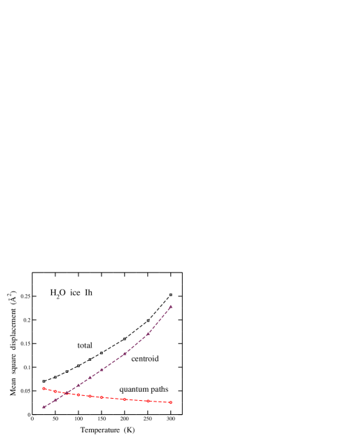
Figure 1: Spatial delocalization of hydrogen nuclei (protons) in H₂O ice Ih, as derived from PIMD simulations at several temperatures. Symbols indicate the mean-square displacement for the centroid $C_{r}^{2}$ (triangles), and the radius-of-gyration of the quantum paths $Q_{r}^{2}$ (circles). The total delocalization $\Delta_{r}^{2}$ is shown by open squares. Lines are guides to the eye.

We first consider the spatial delocalization of hydrogen in normal ice Ih, which is expected to include a nonnegligible quantum contribution. We have calculated separately both terms giving the atomic delocalization in Eq. (3), for each hydrogen atom in the water molecules. In Fig. 1 we display the values of $Q_{r}^{2}$ (spreading of the quantum paths, circles) and $C_{r}^{2}$ (centroid delocalization, triangles), as derived from our PIMD simulations for the H₂O molecule at several temperatures. The total spatial delocalization $\Delta_{r}^{2}$ is shown as squares. In this plot, one observes that at low temperatures the quantum contribution (spreading of the paths), $Q_{r}^{2}$, dominates the spatial delocalization of hydrogen, since the centroid displacement, $C_{r}^{2}$, converges to zero as $T\to 0$ K. The opposite happens at temperatures higher than 70 K, and in the high-temperature limit (unreachable here for stability reasons), the quantum contribution $Q_{r}^{2}$ would eventually disappear, as corresponds to the classical limit. At $T$ = 250 K, close to the melting temperature predicted by this potential model,Ramírez and Herrero (2010) we found $Q_{r}^{2}=2.85\times 10^{-2}$ Ų vs $C_{r}^{2}=0.170$ Ų, i.e., the former contributes a 14% to the total spacial delocalization of hydrogen, $\Delta_{r}^{2}$. We note that at low temperatures the quantum paths associated to hydrogen have an average extension of about 0.15 Å, much smaller than the H–H distance in a water molecule, thus justifying the neglect of quantum exchange between protons in the PIMD simulations.

The mean-square displacement $\Delta_{r}^{2}$ of hydrogen atoms derived from our PIMD simulations with the q-TIP4P/F potential are similar to those derived by Tanaka and MohantyTanaka and Mohanty (2002) from classical molecular dynamics simulations with the TIP4P potential, in the temperature range considered by these authors (from 150 to 250 K). At lower temperatures, classical simulations should give values smaller than the PIMD simulations, due to its neglect of atomic zero-point motion. The atomic mean-square displacements are usually supposed to be related with the melting of a solid. Thus, the Lindemann criterion gives a threshold for the maximum amplitude of atomic vibrations that can be sustained by a crystal. At the melting point of ice Ih we find from our PIMD simulations that this amplitude is about 6% of the H-bond distance, as discussed elsewhere.Ramírez and Herrero (2010)

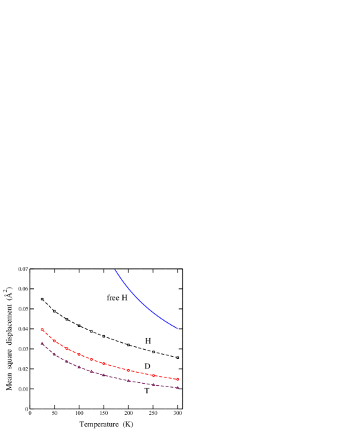
Figure 2: Mean square radius-of-gyration of the quantum paths, $Q_{r}^{2}$, for hydrogen isotopes in ice Ih, as derived from PIMD simulations at several temperatures for H₂O (squares), D₂O (circles), and T₂O (triangles). Error bars are in the order of the symbol size. The solid line represents $Q_{r}^{2}$ for a free hydrogen atom.

Quantum effects are more relevant as the mass of the particles under consideration becomes smaller. Thus, one expects that the quantum delocalization of the hydrogen isotopes in ice will decrease for rising isotopic mass. This is shown in Fig. 2, where we have plotted the mean-square displacement of the quantum paths, $Q_{r}^{2}$, for hydrogen (squares), deuterium (circles), and tritium (triangles) at several temperatures. In the zero-temperature limit and in a harmonic approximation, $Q_{r}^{2}$ is known to scale as $m_{\text{H}}^{-1/2}$. At 25 K, we find a ratio $Q_{r}^{2}$(H)/$Q_{r}^{2}$(D) = 1.39, slightly smaller than the low-temperature harmonic expectancy of $\sqrt{2}$. In the high-temperature limit $Q_{r}^{2}$ goes to zero, but the ratio $Q_{r}^{2}$(H)/$Q_{r}^{2}$(D) converges to the inverse mass ratio,Gillan (1988); Ramírez and Herrero (1993) in this case $m_{\rm D}/m_{\rm H}$ = 2. At 300 K we found $Q_{r}^{2}$(H)/$Q_{r}^{2}$(D) = 1.73, between the high and low-temperature limits. For T₂O we found at 300 K, $Q_{r}^{2}=1.05\times 10^{-2}$ Ų, so that $Q_{r}^{2}$(H)/$Q_{r}^{2}$(T) = 2.44, also between a ratio of $\sqrt{3}$ expected at low temperature in a harmonic approach, and the high-temperature limit given by $m_{\rm T}/m_{\rm H}$ = 3.

For comparison with the results of our PIMD simulations for different hydrogen isotopes in ice Ih, we also present in Fig. 2 the mean-square radius of gyration corresponding to a free hydrogen atom (without any external potential, solid line). This can be calculated analytically, as shown elsewhere,Gillan (1988); Ramírez and Herrero (1993) and gives values of $Q_{r}^{2}$ clearly higher than for hydrogen in ice, in the whole temperature range considered here, confirming the importance of the hydrogen environment in its quantum delocalization. This is even clearly appreciable at the melting temperature.

For the centroid delocalization, $C_{r}^{2}$, of deuterium and tritium in ice Ih we found values almost indistinguishable from those obtained for hydrogen (shown in Fig. 1) in the whole temperature region under consideration, which in turn were practically the same as the mean-square displacement of hydrogen found in classical molecular dynamics simulations.

III.2 Kinetic energy

A typical quantum effect related to the atomic motion in solids is that the kinetic energy $E_{k}$ at low temperature converges to a finite value associated to zero-point motion, contrary to the classical result where $E_{k}$ vanishes at 0 K. Path integral simulations allow one to obtain the kinetic energy of the quantum particles under consideration, which is basically related to the spread of the quantum paths. In fact, for a particle at given temperature and isotopic mass, the larger the mean-square radius-of-gyration of the paths, $Q_{r}^{2}$, the smaller the kinetic energy. Here we have calculated $E_{k}$ by using the so-called virial estimator, which has an associated statistical uncertainty lower than the potential energy of the system.Herman et al. (1982); Tuckerman and Hughes (1998)

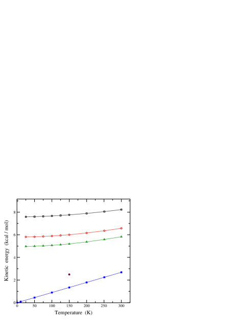
Figure 3: Temperature dependence of the kinetic energy of ice Ih, as derived from PIMD simulations. Open symbols indicate results derived from simulations with full quantum motion of the atoms in the cell: squares for H₂O, circles for D₂O, and triangles for T₂O. For comparison we also present results of classical molecular dynamics simulations (filled squares). The filled circle corresponds to a PIMD simulation of ice with the hydrogen mass going to infinity. Error bars are less than the symbol size. Lines are guides to the eye.

In Fig. 3 we display the kinetic energy as a function of temperature for ice Ih. Open symbols indicate results derived from PIMD simulations: H₂O (squares), D₂O (circles), and T₂O (triangles). In each case, $E_{k}$ increases as temperature rises, and at low temperature it converges to the value corresponding to zero-point motion. At a given temperature, $E_{k}$ decreases for increasing isotopic mass. Thus, at $T$ = 25 K we obtained $E_{k}$ = 7.59, 5.81, and 4.98 kcal/mol for H₂O, D₂O, and T₂O, respectively. The change in kinetic energy caused by isotopic substitution decreases as temperature is raised. However, we stress that at the melting temperature, the kinetic energy of deuterated ice is still more than 1.5 kcal/mol lower than that of normal ice, reflecting the importance of quantum effects in ice Ih at this temperature.

For comparison with the results of our PIMD simulations, we also present in Fig. 3 the kinetic energy corresponding to a classical model with $3N$ degrees of freedom ($N$ atoms): $E_{k}^{\text{c}l}=3Nk_{B}T/2$, solid squares. For rising temperature, the classical kinetic energy approaches the results of the PIMD simulations, in particular those corresponding to the heaviest molecule, T₂O. However, at 300 K the classical value is still lower than $E_{k}$(T₂O) by 3.14 kcal/mol, which represents about 50% of the quantum value. To assess the importance of quantum effects associated to the oxygen motion, we also show in Fig. 3 the kinetic energy obtained in PIMD simulations at 150 K for the limit $m_{\text{H}}\to\infty$. In this case we obtain $E_{k}$ = 2.49 kcal/mol, i.e. 1.15 kcal/mol above the classical limit at this temperature. This represents about 30% of the increase in kinetic energy from the classical limit to T₂O quantum ice.

III.3 Crystal volume

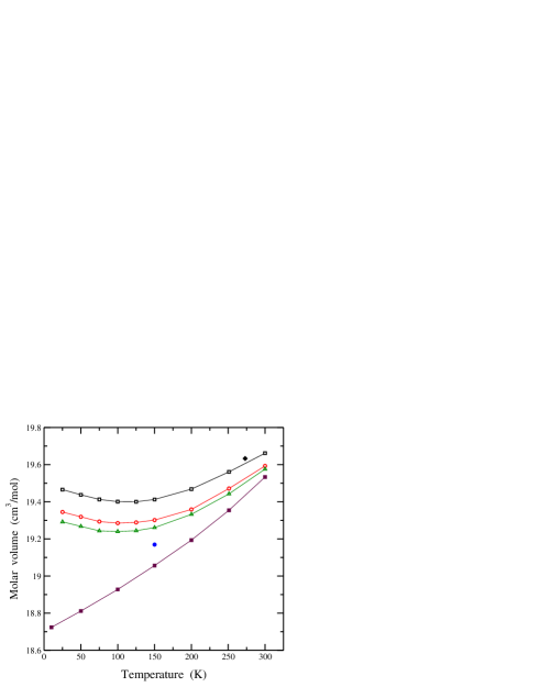
Figure 4: Molar volume of ice Ih as a function of temperature, as derived from PIMD simulations for H₂O (squares), D₂O (circles), and T₂O (triangles). For comparison, results of classical molecular dynamics simulations (filled squares) are also shown. A filled circle corresponds to the ice volume obtained from a PIMD simulation with the hydrogen mass going to infinity. Error bars are in the order of the symbol size. Lines are guides to the eye. A solid diamond represents the experimental determination from Refs. Ginnings and Corruccini, 1947; Dantl and Gregora, 1968 at 273 K.

As commented in the Introduction, the crystal volume is expected to change with the isotopic mass of the constituent atoms. We have calculated the equilibrium volume of ice Ih in our isothermal-isobaric PIMD simulations for different hydrogen masses. In Fig. 4 we present the temperature dependence of the molar volume for the different isotopes. Results of our PIMD simulations at $P$ = 1 bar are shown as open symbols: H₂O (squares), D₂O (circles), and T₂O (triangles). One first notices that the change of volume with temperature is not monotonic, but at low temperatures it decreases as temperature is raised, to reach a minimum at $T\approx 100$ K. At higher temperature, the molar volume increases, and the solid recovers the usual thermal expansion. Also, the volume of the solid decreases as the isotope mass of hydrogen is raised, as a consequence of the smaller spatial (quantum) delocalization associated to a larger nuclear mass. We observe for all three isotopes the same behavior of the volume, with a minimum around 100 K. The volume changes derived from the PIMD simulations are isotropic, i.e., the ratio between parameters of the simulation cell is constant when changing the temperature, within the statistical error bar, which agrees with experimental data.Röttger et al. (1994) For thermodynamic reasons, one expects that in the low-temperature limit ($T\to 0$ K) the thermal expansion of the solid goes to zero, i.e., $dV/dT\to 0$. We cannot, however, check this point at present since PIMD simulations at temperatures lower than 25 K would require enormous computational resources.

The molar volume (or density) of ice has been determined experimentally in very different ways, e.g., calorimetric, acoustical, mechanical, x-ray, optical, or nuclear methods (see Feistel and Wagner, 2006 and references therein). Measurements of different authors typically deviate from each other by up to about 0.3%, which could be caused by the density lowering effect of aging on ice crystals or by their very slow relaxation to equilibrium.Feistel and Wagner (2006) The molar volumes 19.635 cm³/mol of Ginnings and CorrucciniGinnings and Corruccini (1947) and 19.633 cm³/mol of Dantl and GregoraDantl and Gregora (1968) are considered in Ref. Feistel and Wagner, 2006 the most accurate determinations at normal pressure and 273 K. They are plotted in Fig. 4 as a solid diamond. At lower temperatures, there appears some dispersion in the experimental points presented by different authors. A minimum in the molar volume was found in several worksDantl (1962); Röttger et al. (1994); Feistel and Wagner (2006) in the range between 60 and 90 K, to be compared with the minimum at around 100 K derived from our PIMD simulations. The minimum molar volume was found to be around 19.3 cm³/mol, somewhat smaller than our calculated value at 100 K (19.40 cm³/mol). This, along with the rather good agreement between calculated and experimental values at the melting temperature, indicates that the employed interatomic potential underestimates the thermal expansion of the solid. In this context, the most remarkable point is that the q-TIP4P/F potential is able to capture the negative thermal expansion of ice at low temperatures. This phenomenon is associated to the tetrahedral coordination of the water molecules in ice, and has been observed in other solids with similar structures. In particular, it is well known for crystals with diamond and zinc blende structure, such as Si, GaAs, and CuCl.Evans (1999)

Another important point to be stressed here is the appreciable isotopic effect on the molar volume. In fact, at $T$ = 100 K, we found $v$ = 19.400, 19.285, and 19.240 cm³/mol, for H₂O, D₂O, and T₂O, respectively, which translates into a volume reduction of 0.6% and 0.8% in passing from normal ice to deuterated and tritiated ice, respectively. From the crystal structure obtained by Röttger et al.Röttger et al. (1994) one derives for normal ice Ih at 100 K a molar volume of 19.301 cm³/mol, somewhat smaller than that found in the PIMD simulations with the q-TIP4P/F potential. These authors also measured the lattice parameters of deuterated ice, and found an inverse isotopic effect, which is not reproduced in our simulations.

For comparison, we also present in Fig. 4 the molar volume of ice Ih derived from classical molecular dynamics simulations with the same interatomic potential (filled squares). At a given temperature, the volume obtained from the classical simulations is smaller than that found in quantum PIMD simulations, but the difference decreases as $T$ rises. Note that, contrary to the results of the quantum simulations, the molar volume obtained in the classical ones increases monotonically and does not show any anomaly in the whole temperature region up to 300 K. At $T$ = 100 K, we obtain in the classical approximation a molar volume $v$ = 18.928 cm³/mol. This means that at this temperature, quantum effects cause for normal ice Ih a remarkable volume expansion of about 2.5%. In the zero-temperature limit one can estimate for H₂O ice a volume increase of about 0.8 cm³/mol, which means a rise around 4.3% due to nuclear quantum effects.

We note that both the thermal expansion (positive or negative) and the isotopic effect on the crystal volume are anharmonic effects that would be absent in a harmonic approximation. On one side, the thermal expansion appears in both classical and quantum simulations, since in both cases the atomic vibrations feel the anharmonicity of the interatomic potential at any finite temperature ($T>$ 0 K). In the quantum case, the anharmonicity is also felt in the low-temperature limit $T\to 0$ K, due to zero-point motion, and thus in this limit the crystal volume is larger for quantum than for classical calculations (which may be called “zero-point crystal expansion”). On the other side, the isotopic effect on the crystal volume is a typical quantum effect that disappears in the classical limit, and is associated to the different vibrational amplitudes of different isotopes (which coincide in the classical limit).

The negative thermal expansion of ice at low $T$ is due to low-energy transverse vibrational modes with negative Grüneisen parameter. For a mode in the $n$’th phonon branch with wave vector ${\bf q}$, this parameter $\gamma_{n}({\bf q})$ is defined from the logarithmic derivative of its frequency with respect to the crystal volume:Ashcroft and Mermin (1976)

$$\gamma_{n}({\bf q})=-\frac{\partial\ln\omega_{n}({\bf q})}{\partial\ln V}\,.$$ (6)

At relatively low temperature, low-energy modes are more populated than modes with higher energy (with positive $\gamma_{n}({\bf q})$), and then the overall contribution to the volume change with increasing temperature will be negative.Tanaka (1998); Bennington et al. (1999) In this line, Tanaka calculated the temperature dependence of the crystal volume in a quasiharmonic approximation and obtained a negative thermal expansion at low temperatures.Tanaka (1998, 2001) This author calculated the relative weight of different vibrational modes to the overall thermal expansion at different temperatures, and found that a family of low energy modes ($\omega<$ 50 cm^-1), corresponding to bending motion of three water molecules is largely responsible for the negative thermal expansion at low temperatures. In connection with this, an instability in a transverse acoustical mode in ice Ih was found at low temperature from incoherent inelastic neutron scattering.Bennington et al. (1999)

We remember that in the classical molecular dynamics simulations of ice Ih we did not obtain any negative thermal expansion, in contrast with PIMD simulations. This is in line with the explanation given above related to the different weight of phonons with different energies at low temperatures. In a classical model all phonons have the same weight at any temperature (equipartition principle), and thus the negative Grüneisen parameter of low-energy transverse modes is largely compensated for at any temperature by the positive $\gamma$ of most vibrational modes in the solid.

It is worthwhile commenting on the effect of pressure upon the molar volume of ice. It is well known that ice Ih is no longer mechanically stable at pressures in the order of 1 GPa, where it has been observed to transform into an amorphous phase.Mishima et al. (1984); Sciortino et al. (1995) This has been in fact obtained in our PIMD simulations at $T=$ 251 K and $P=$ 1 GPa, where the ice crystal collapsed into an amorphous solid, with a volume decrease of about 18%. At $P=$ 0.8 GPa and the same temperature we found that the ice crystal was still stable along our simulation runs, and obtained a reduction in the crystal volume of 8.1% with respect to ambient pressure. Interestingly, at 0.8 GPa the atomic delocalization of hydrogen was found to be $\Delta_{r}^{2}$ = 0.309 Ų, to be compared with a value of 0.199 Ų obtained at $P=$ 1 atm (see above), which means a large increase in the mean-square displacement of about 50%. Such an anomalous increase in the atomic delocalization seems to be related with the crystal instability associated to the amorphization of ice Ih under pressure. This question requires further investigation by using path-integral simulations at different pressures.

III.4 Interatomic distances

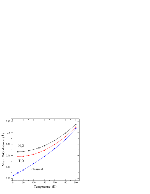
Figure 5: Mean distance between oxygen atoms in nearest-neighbor water molecules, as a function of temperature. Open symbols correspond to results of PIMD simulations for H₂O (squares) and T₂O (triangles). Filled squares represent results of classical molecular dynamics simulations. Lines are guides to the eye.

In this subsection we present results for interatomic distances in ice Ih between atoms in the same and adjacent molecules. We first show in Fig. 5 the mean distance between oxygen atoms in neighboring molecules. Open symbols represent results of PIMD simulations: squares for H₂O and triangles for T₂O. Data points for the case of D₂O lie between those of H₂O and T₂O, and are not shown for clarity. For comparison we also present in this figure the average O–O distance derived from classical molecular dynamics simulations (filled squares). Comparing results of PIMD and classical simulations, we find that in the low-temperature limit the O–O distance for normal ice increases by about 0.04 Å with respect to the classical value, i.e., around 1.5%. The O–O distance derived from quantum simulations increases as temperature is raised, and the slope rises from a vanishing value at $T\to 0$ K to nearly the classical value at 300 K. For tritiated ice we found an interatomic distance between that for H₂O ice and the classical limit.

For a totally homogeneous and isotropic crystal expansion one expects a volume change $\Delta V/V=3\Delta l/l$, $l$ being any distance in the solid. This relation is valid for small volume changes, i.e., for $\Delta V/V\ll 1$, as occurs in the temperature range considered here, and in particular, one would expect it to be fulfilled for the intermolecular distance in the solid. Thus, from the increase in the average O–O distance at low temperature for ice Ih one expects a volume expansion of about 4.5% due to zero-point motion. This value is close to that estimated from the volumes obtained in classical and quantum simulations at low temperature, which give an expansion of 4.3% (see above, Sec. III.C). Note, however, that a fixed relation between interatomic distances and crystal volume can not be strictly followed in the case of ice Ih when the temperature is raised, specially in the region where the crystal shrinks. In fact, we observe that the average O–O distance does not present a minimum at $T\approx$ 100 K, as the molar volume of ice. This clearly reflects the fact that shrinking of the ice crystal is not due to a reduction in the distance between nearest molecules, but to a bending motion of contiguous molecules, corresponding to low-frequency vibrational modes, as indicated above in Sec. III.C. From the results of our quantum and classical simulations at 100 K we find a volume increase of 2.5% due to quantum nuclear effects vs a relative rise of 0.9% in the average O–O distance, which would correspond to a volume change of 2.7% for an isotropic and homogeneous expansion.

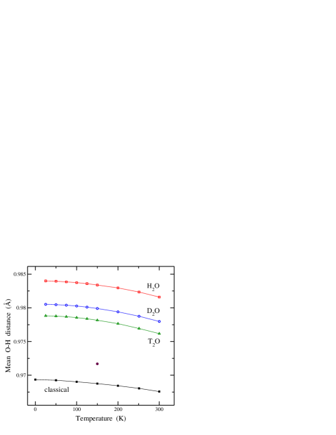
Figure 6: Temperature dependence of the mean intramolecular O–H distance, as derived from simulations of ice Ih. Open symbols represent results of PIMD simulations for H₂O (squares), D₂O (circles), and T₂O (triangles). For comparison, the average O–H distance obtained from classical molecular dynamics simulations (filled squares) are also presented. The filled circle corresponds to the limit $m_{\text{H}}\to\infty$ in PIMD simulations. Error bars are in the order of the symbol size. Lines are guides to the eye.

We now turn to analyze the interatomic distances inside water molecules in the ice crystal, as derived from our simulations at different temperatures. In Fig. 6 we have plotted the mean intramolecular O–H distance as a function of temperature. As in previous figures, open symbols indicate results of PIMD simulations for H₂O (squares), D₂O (circles), and T₂O (triangles). At a given temperature, the average O–H distance is larger for smaller hydrogen isotopic mass. In particular, the difference between O–H and O–D distances amounts to about $4\times 10^{-3}$ Å in the whole temperature range under consideration, which agrees with data derived from Compton scattering experiments for water at room temperature.Nygård et al. (2007) For comparison, we present in Fig. 6 results for the classical limit (filled squares), which lie clearly lower than those of the quantum simulations. To assess the relative importance of quantum nuclear effects of hydrogen and oxygen, we give also the O–H distance obtained in a PIMD simulation in the limit of infinite hydrogen mass (filled circle at 150 K). This point is still clearly above the classical limit, with a quantum contribution (coming from quantum delocalization of oxygen nuclei) amounting to 31% and 20% of the increase in O–H distance for full quantum T₂O and H₂O ice, respectively.

It is interesting that the intramolecular O–H distance decreases for increasing temperature, in both classical and quantum approaches. This fact has been observed experimentally and reported in the literature.Nygård et al. (2006) It is due to the peculiar structure of ice with hydrogen bonds connecting neighboring water molecules. As temperature is raised, molecular motion is enhanced, so that hydrogen bonds become softer, and the average intermolecular O–H distance rises (in agreement with the increase in O–O distance presented above). This causes a strengthening of the intramolecular O–H bonds, with a concomitant decrease in the interatomic distance in water molecules. The same behavior is found from the classical molecular dynamics simulations (filled squares in Fig. 6), although in this case the mean intramolecular O–H distance is clearly smaller than in the full quantum ice.

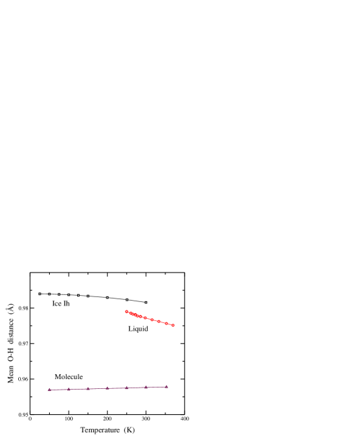
Figure 7: Temperature dependence of the average intramolecular O–H distance, as derived from PIMD simulations of a single H₂O molecule (triangles), ice Ih (squares), and liquid water (circles). Error bars are in the order of the symbol size. Lines are guides to the eye.

To obtain deeper insight into the contraction of the intramolecular O–H bond for rising temperature, we compare in Fig. 7 the average O–H distance derived from our PIMD simulations for ice Ih (open squares) with those obtained for liquid water (circles) and for an isolated H₂O molecule (triangles). One observes first that the O–H distance in the water molecules increases appreciably in passing from the gas phase to condensed phases (solid and liquid). This is a consequence of hydrogen bonds with the nearest molecules, which weaken the intramolecular bonds. The enlargement of these intramolecular bonds is larger for the solid than for the liquid, since in the former the intermolecular hydrogen bonds are stronger due to the lower mobility of the molecules and the larger rigidity of the H-bond network. In the case of ice Ih, the bond enlargement with respect to an isolated H₂O molecule amounts to about 0.03 Å, which means a 3% of the bond distance. Second, one observes that the O–H distance for an isolated molecule increases slightly as the temperature is raised, contrary to the condensed phases, where this distance decreases for increasing temperature. The behavior observed for the isolated molecule is the usual thermal expansion due to anharmonicities in the interatomic potential. For the condensed phases, this natural expansion is largely compensated for by intermolecular interactions through hydrogen bonds, as indicated above. As a result, the intramolecular O–H distance in these phases decreases as the temperature rises.

III.5 Bulk modulus

Among the many surprising properties of liquid water and ice, one finds that their compressibility is smaller than what one could naively expect from the large cavities present in their structure, which could presumably collapse under pressure without water molecules approaching close enough to repel each other. For ice Ih, in particular, the hydrogen bonds holding the crystal structure are rather stable, as manifested by the relatively high pressure necessary to break down the H-bond network and amorphize the solid.Sciortino et al. (1995)

The isothermal compressibility $\kappa$ of ice, or its inverse the bulk modulus [$B=1/\kappa=-V({\partial P}/{\partial V})_{T}$] can be calculated directly from our PIMD simulations in the isothermal-isobaric ensemble. In fact, in the $NPT$ ensemble the isothermal bulk modulus can be obtained from the mean-square fluctuations of the volume, $\sigma_{V}^{2}=\langle V^{2}\rangle-\langle V\rangle^{2}$, by using the expressionLandau and Lifshitz (1980); Herrero (2008)

$$B=\frac{k_{B}T\langle V\rangle}{\sigma_{V}^{2}}\;,$$ (7)

where $k_{B}$ is Boltzmann’s constant. This expression has been employed earlier to calculate the bulk modulus of different types of solids from path-integral simulations.Herrero and Ramírez (2001); Herrero (2008) Here, we have used Eq. (7) to obtain $B$ for ice Ih from both classical and PIMD simulations.

In the classical simulations we find that the bulk modulus decreases roughly linearly as temperature is raised, and in the zero-temperature limit it extrapolates to a value $B_{0}=17.6\pm 0.3$ GPa. In the quantum simulations of H₂O ice Ih, the solid is found to be “softer” than in the classical simulations, in the sense that in the former the volume fluctuations are larger, and consequently the bulk modulus becomes smaller. Note that in Eq. (7) one also has the average volume $\langle V\rangle$ in the numerator, which is larger for the quantum than for the classical solid (see Sec. III.C), but this volume increase due to quantum nuclear effects is dominated by the also present larger volume fluctuations $\sigma_{V}^{2}$. In the low-temperature limit we find an extrapolated value of $B=13.8\pm 0.4$ GPa, about 3.8 GPa smaller than the classical value, which means that the quantum effect reduces the bulk modulus by more than 25%.

Note that the values of $B$ derived from our simulations in the isothermal-isobaric ensemble show relative error bars larger than those corresponding to other calculated variables (e.g., kinetic energy, interatomic distances, or molar volume). This is a consequence of the statistical uncertainty of the volume fluctuations $\sigma_{V}$, that are employed to calculate the bulk modulus $B$. The error bars are similar for both classical and PIMD simulations.

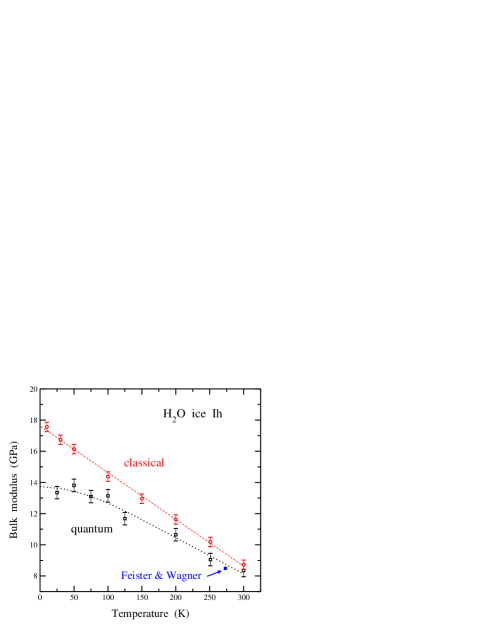
Figure 8: Bulk modulus of ice Ih as obtained from quantum PIMD (open squares) and classical molecular dynamics (open circles) simulations for H₂O. Error bars show the statistical uncertainty in the values of $B$ found from the simulations. The filled square corresponds to the value obtained at 273 K from the equation of state derived by Feistel and WagnerFeistel and Wagner (2006) from experimental data. Lines are guides to the eye.

There appears in the literature a dispersion of data for the isothermal compressibility (or bulk modulus) of ice Ih at the melting temperature and normal pressure. The bulk modulus of ice found from our PIMD simulations is close to that derived by Feistel and Wagner,Feistel and Wagner (2006) who obtained an equation of state for ice Ih from a set of experimental data. This value at 273 K is shown in Fig. 8 as a solid square. It is hard to estimate the precision of this value of the bulk modulus due to lack of error bars for the published data, and the uncertainty may be large, as suggested by the dispersion in the experimental data obtained by different authors. The uncertainty is even larger at lower temperatures, where we could not find direct experimental data. From the equation of state by Feistel and WagnerFeistel and Wagner (2006) one derives at low temperature and normal pressure an isothermal bulk modulus of 10.6 GPa, somewhat lower than the low-temperature extrapolation of our simulation results.

The bulk moduli for D₂O and T₂O ice derived from our PIMD simulations show a similar trend to that of normal ice Ih, and have not been presented in Fig. 8 for clarity. They seem to lie between the classical limit and the quantum value for H₂O, but due to the data dispersion, the difference between $B$ values for the different hydrogen isotopes can be hardly quantified. Moreover, we do not observe in the bulk modulus of ice any anomaly similar to that of the crystal volume at $T\approx 100$ K, but we cannot exclude it from our present results because of their statistical uncertainty.

IV Summary

We have presented results of PIMD simulations of ice Ih with different hydrogen isotopes in a wide range of temperatures. This technique allows us to explore readily isotope effects, since the atomic masses appear as input parameters in the calculations. This kind of simulations enable one to calculate separately kinetic and potential energies at finite temperatures, taking into account the quantization of nuclear motion. This includes consideration of zero-point motion of the atoms in the solid, which can be hard to analyze by analytical calculations in the presence of light atoms and large anharmonicities.

This kind of quantum simulations are necessary to reproduce some observed facts of ice, that are not captured by classical simulations. In this sense, PIMD simulations with the q-TIP4P/F potential are able to reproduce the negative thermal expansion of ice Ih at low temperatures. Also, these simulations reproduce the apparently anomalous decrease of the intramolecular O–H distance for increasing temperature. A good check of the employed interatomic potential is the calculation of a macroscopic observable such as the bulk modulus, which has been accurately reproduced in our calculations. Note that the use of a flexible potential model for water has allowed us to look in a realistic way at changes in the intramolecular O–H distance and quantum delocalization of hydrogen at different temperatures.

PIMD simulations give reliable predictions for several isotope effects in condensed matter. For ice Ih, in particular, we have seen how the isotopic mass of hydrogen affects the kinetic energy and atomic delocalization in the crystal, as well as the interatomic distances and molar volume. Thus, we found for D₂O ice Ih at 100 K a decrease in the crystal volume and intramolecular O–H distance of 0.6% and 0.4%, respectively, as compared to H₂O ice. Our simulations, however, do not reproduce the inverse isotopic effect in the crystal volume, observed in Ref. 43.

Simulations similar to those presented here can be carried out for ice under an external pressure, and in particular to study the amorphization process of the ice crystal. Also, the question of quantum tunneling and diffusion of hydrogen in the different ice structures needs further investigation. These are challenging problems that could be addressed in the near future by using path-integral simulations.