Triangulations of Cayley and Tutte polytopes

Abstract.

Cayley polytopes were defined recently as convex hulls of Cayley compositions introduced by Cayley in 1857. In this paper we resolve Braun’s conjecture, which expresses the volume of Cayley polytopes in terms of the number of connected graphs. We extend this result to two one-variable deformations of Cayley polytopes (which we call $t$-Cayley and $t$-Gayley polytopes), and to the most general two-variable deformations, which we call Tutte polytopes. The volume of the latter is given via an evaluation of the Tutte polynomial of the complete graph.

Our approach is based on an explicit triangulation of the Cayley and Tutte polytope. We prove that simplices in the triangulations correspond to labeled trees. The heart of the proof is a direct bijection based on the neighbors-first search graph traversal algorithm.

1. Introduction

In the past several decades, there has been an explosion in the number of connections and applications between Geometric and Enumerative Combinatorics. Among those, a number of new families of “combinatorial polytopes” were discovered, whose volume has a combinatorial significance. Still, whenever a new family of $n$-dimensional polytopes is discovered whose volume is a familiar integer sequence (up to scaling), it feels like a “minor miracle”, a familiar face in a crowd in a foreign country, a natural phenomenon in need of an explanation.

In this paper we prove a surprising conjecture due to Ben Braun [BBL], which expresses the volume of the Cayley polytope in terms of the number of connected labeled graphs. Our proof is robust enough to allow generalizations in several directions, leading to the definition of Tutte polytopes, and largely explaining this latest “minor miracle”.

We start with the following classical result.

Theorem 1.1 (Cayley, 1857)

The number of integer sequences $(a_{1},\ldots,a_{n})$ such that $1\leq a_{1}\leq 2$, and $1\leq a_{i+1}\leq 2\hskip 0.85355pta_{i}$ for $1\leq i<n$, is equal to the total number of partitions of integers $N\in\{0,1,\ldots,2^{n}-1\}$ into parts $1,2,4,\ldots,2^{n-1}$.

Although Cayley’s original proof [Cay] uses only elementary generating functions, it inspired a number of other proofs and variations [APRS, BBL, CLS, KP]. It turns out that Cayley’s theorem is best understood in a geometric setting, as an enumerative problem for the number of integer points in an $n$-dimensional polytope defined by the inequalities as in the theorem.

Formally, following [BBL], define the Cayley polytope ${{\text{\hskip 0.85355pt\bf{C}}}}_{n}\subset\mathbb{R}^{n}$ by inequalities:

$$1\hskip 1.70709pt\leq\hskip 1.70709ptx_{1}\hskip 1.70709pt\leq 2\hskip 0.85355pt,\ \ \text{and}\ \hskip 1.70709pt1\hskip 1.70709pt\leq\hskip 1.70709ptx_{i}\hskip 1.70709pt\leq\hskip 1.70709pt2\hskip 0.85355ptx_{i-1}\,\mbox{ for }\ i\hskip 0.85355pt=\hskip 0.85355pt2,\ldots,n\hskip 0.85355pt,$$

so that the number of integer points in ${{\text{\hskip 0.85355pt\bf{C}}}}_{n}$ is the number of integer sequences $(a_{1},\ldots,a_{n})$, and the number of certain partitions, as in Cayley’s theorem.

In [BBL], Braun made the following interesting conjecture about the volume of ${{\text{\hskip 0.85355pt\bf{C}}}}_{n}$. Denote by $\mathcal{C}_{n}$ the set of connected graphs on $\hskip 0.85355ptn\hskip 0.85355pt$ nodes, and let $C_{n}=\bigl{|}\mathcal{C}_{n}\bigr{|}$.

Theorem 1.2 (Formerly Braun’s conjecture)

Let ${{\text{\hskip 0.85355pt\bf{C}}}}_{n}\subset\mathbb{R}^{n}$  be the Cayley polytope defined above. Then  ${\text{\rm vol}}\hskip 0.85355pt{{\text{\hskip 0.85355pt\bf{C}}}}_{n}=C_{n+1}/n!$.

This result is the first in a long chain of results we present in this paper, leading to the following general result. Let $0<q\leq 1$ and $t\geq 0$. Define the Tutte polytope ${{\text{\hskip 0.85355pt\bf{T}}}}_{n}(q,t)\subset\mathbb{R}^{n}$ by inequalities: $x_{n}\geq 1-q$ and

$$(\diamond)\hskip 22.76228ptq\hskip 0.85355ptx_{i}\,\leq\,q\hskip 0.85355pt(1+t)\hskip 0.85355ptx_{i-1}\hskip 1.70709pt-\hskip 1.70709ptt\hskip 0.85355pt(1-q)(1-x_{j-1})\hskip 0.85355pt,$$

where $1\leq j\leq i\leq n$ and $x_{0}=1$.

Theorem 1.3 (Main result)

Let ${{\text{\hskip 0.85355pt\bf{T}}}}_{n}(q,t)\subset\mathbb{R}^{n}$  be the Tutte polytope defined above. Then

$${\text{\rm vol}}\hskip 0.85355pt{{\text{\hskip 0.85355pt\bf{T}}}}_{n}(q,t)\,=\,t^{n}{\text{\rm T}}_{K_{n+1}}(1+q/t,1+t)\hskip 0.85355pt/n!,$$

where ${\text{\rm T}}_{H}(x,y)$ denotes the Tutte polynomial of graph $H$.

One can show that in certain sense, Tutte polytopes are a two variable deformation of the Cayley polytope:

$$\lim_{q\to 0+}\hskip 1.70709pt{{\text{\hskip 0.85355pt\bf{T}}}}_{n}(q,1)\,=\,{{\text{\hskip 0.85355pt\bf{C}}}}_{n}\hskip 0.85355pt.$$

To see this, note that for $t=1$, the inequalities with $j=1$ in $(\diamond)$ give $x_{i}\leq 2x_{i-1}$, and for $j>1$, we get $x_{j-1}\geq 1$ as $q\to 0+$.

Now, recall that ${\text{\rm T}}_{H}(1,2)$ is the number of connected subgraphs of $H$, a standard property of Tutte polynomials (see e.g. [Bol]). Letting $q\to 0+$ and $t=1$ shows that Theorem 1.3 follows immediately from Theorem 1.2. In other words, our main theorem is an advanced generalization of Braun’s Conjecture (now Theorem 1.2).

The proof of both Theorem 1.2 and 1.3 is based on explicit triangulations of polytopes. The simplices in the triangulations have a combinatorial nature, and are in bijection with labeled trees (for the Cayley polytope) and forests (for the Tutte polytope) on $n+1$ nodes. This bijection is based on a variant of the neighbors-first search (NFS) graph traversal algorithm studied by Gessel and Sagan [GS]. Roughly speaking, in the case of Cayley polytopes, the volume of a simplex in bijection with a labeled tree $T$ corresponds to the set of labeled graphs for which $T$ is the output of the NFS.

To be more precise, our most general construction gives two subdivisions of the Tutte polytope, a triangulation (subdivision into simplices) and a coarser subdivision that can be obtained from simplices with products and coning. Some (but not all) of the simplices involved are Schläfli orthoschemes (see below). The polytopes in the coarser subdivision are in bijection with plane forests, so there are far fewer of them. In both subdivisions, the volume of the simplex or the polytope in bijection with a forest $F$ on $n+1$ nodes, times $n!$, is equal to the generating function of all the graphs $G$ that map into it by the number of connected components (factor $q^{k(G)-1}$) and the number of edges (factor $t^{|E(G)|}$).

Rather than elaborate on the inner working of the proof, we illustrate the idea in the following example.

Example 1.4

The triangulation of ${\text{\rm T}}_{2}(q,t)$ is shown on the left-hand side of Figure 1. For example, the top triangle is labeled by the tree with edges $12$ and $13$; its area, multiplied by $2!$, is $t^{2}(1+t)$, and it also has two graphs that map into it, the tree itself (with two edges) and the complete graph on $3$ nodes (with three edges). The coarser subdivision is shown on the right-hand side of Figure 1. The bottom rectangle corresponds to the plane forest with two components, the first having two nodes. Its area, multiplied by $2!$, is $2qt$, and there are indeed two graphs that map into it, both with two components (and hence a factor of $q$) and one edge (and hence a factor of $t$). Triangulation of ${\text{\rm T}}_{3}(q,t)$ is shown in Figure 2.

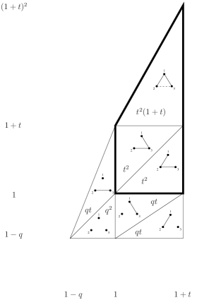
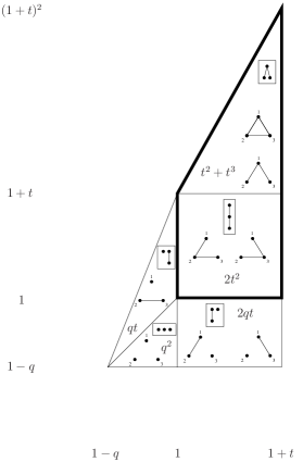
Figure 1. A triangulation and a subdivision of the Tutte polytope $\mathbf{T}_{2}(q,t)$.

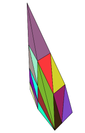
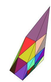
Figure 2. A triangulation of the Tutte polytope $\mathbf{T}_{3}(q,t)$ from two angles.

The rest of the paper is structured as follows. We begin with definitions and basic combinatorial results in Section 2. In Sections 3 and 4 we construct a triangulation and a coarse subdivision of the Cayley polytope. In Section 5 we present a similar construction for what we call the Gayley polytope, which can be defined as a special case of the Tutte polytope $\mathbf{T}_{n}(1,1)$. Two one parametric families of deformations of Cayley and Gayley polytopes are then considered in Section 6; we call these $t$-Cayley and $t$-Gayley polytopes. Tutte polytopes are then defined and analyzed in Section 7. The vertices of the polytopes are studied in Sections 8. An ad hoc application of the volume of $t$-Cayley polytopes to the study of inversion polynomials is given in Section 9. We illustrate all constructions with examples in Section 10. The proofs of technical results in Sections 3$-$8 appear in the lengthy Section 11. We conclude with final remarks and open problems in Section 12.

2. Combinatorial and geometric preliminaries

2.1.

A labeled tree is a connected acyclic graph. We take each labeled tree to be rooted at the node with the maximal label. A labeled forest is an acyclic graph. Its components are labeled trees, and we root each of them at the node with the maximal label. Cayley’s formula states that there are $n^{n-2}$ labeled trees on $n$ nodes. An unlabeled plane forest is a graph without cycles in which we do not distinguish the nodes, but we choose a root in each component, which is an unlabeled plane tree, and the subtrees at any node, as well as the components of the graph, are linearly ordered (from left to right). The number of plane forests on $n$ nodes is the $n$-th Catalan number $\operatorname{Cat}(n)=\frac{1}{n+1}\binom{2n}{n}$, and the number of plane tree on $n$ nodes is $\operatorname{Cat}(n-1)$. The degree of a node in a plane forest is the number of its successors, which is the usual (graph) degree if the node is a root, and one less otherwise. The depth-first traversal goes through the forest from the left-most tree to the right; within each tree, it starts at the root, and if nodes $v$ and $v^{\prime}$ have the same parent and $v$ is to the left of $v^{\prime}$, it visits $v$ and its successors before $v^{\prime}$.

The degree sequence of a tree $T$ on $n$ nodes is the sequence $(d_{1},\ldots,d_{n})$ where $d_{i}$ is the degree of the $i$-th node in depth-first traversal. Since the last node is a leaf, the degree sequence always ends with a zero. The degree sequence determines the plane tree uniquely, and we have $\sum_{i=1}^{n}d_{i}=n-1$. The degree sequence of a forest $F$ is the concatenation of the degree sequences of its components, and it determines the plane forest uniquely. Finally, if we erase zeros marking the ends of components, we get a reduced degree sequence. We refer to [Sta3, § 5.3 and Exc. 6.19e] for further details.

2.2.

For a (multi)graph $G$ on the set of nodes $V$, denote by $k(G)$ the number of connected components of $G$, and by $e(G)$ the number of edges of $G$. Consider a polynomial

$${\text{\rm Z}}_{G}(q,t)\hskip 1.70709pt=\hskip 1.70709pt\sum_{H\subseteq G}q^{k(H)-k(G)}t^{e(H)},$$

where the sum is over all spanning subgraphs $H$ of $G$. This polynomial is a statistical sum in the random cluster model in statistical mechanics. It is related to the Tutte polynomial

$${\text{\rm T}}_{G}(x,y)\hskip 1.70709pt=\hskip 1.70709pt\sum_{H\subseteq G}(x-1)^{k(H)-k(G)}(y-1)^{e(H)-|V|+k(H)}$$

by the equation

$${\text{\rm T}}_{G}(x,y)\hskip 1.70709pt=\hskip 1.70709pt(y-1)^{k(G)-|V|}\hskip 1.70709pt{\text{\rm Z}}_{G}((x-1)(y-1),y-1)\hskip 0.85355pt.$$

Tutte’s classical result is a combinatorial interpretation for coefficients of the Tutte polynomial [Tut]. He showed that for a connected graph $G$ we have:

$$(\lozenge)\ \ \ {\text{\rm T}}_{G}(x,y)\hskip 1.70709pt=\hskip 1.70709pt\sum_{T\in G}\hskip 0.85355ptx^{\operatorname{ia}(T)}\hskip 0.85355pty^{\operatorname{ea}(T)}\hskip 1.70709pt,$$

where the summation is over all spanning trees $T$ in $G$; here $\operatorname{ia}(T)$ and $\operatorname{ea}(T)$ denote the number of internally active and externally active edges in $T$, respectively. While both $\operatorname{ia}(T)$ and $\operatorname{ea}(T)$ depend on the ordering of the edges in $G$, the sum $(\lozenge)$ does not (see [Bol, §X.5] for definitions and details).

For the complete graph $K_{n}$, the Tutte polynomial and its evaluations are well studied (see [Tut, Ges2]). In this case, under a lexicographic ordering of edges, the statistics $\operatorname{ia}(T)$ and $\operatorname{ea}(T)$ can be interpreted combinatorially [Ges2, GS] via the neighbor-first search (NFS) introduced in [GS], a variant of which is also crucial for our purposes. Take a labeled connected graph $G$ on $n+1$ nodes. Choose the node with the maximal label, i.e. $n+1$, as the first active node (and also the $0$-th visited node). At each step, visit the previously unvisited neighbors of the active node in decreasing order of their labels, and make the one with the smallest label the new active node. If all the neighbors of the active node have been visited, backtrack to the last visited node that has not been an active node, and make it the new active node. The resulting search tree $T$ is a labeled tree on $n+1$ nodes, we denote it $\Phi(G)$ (see Example 10.1).

In a special case, the polynomial $\operatorname{Inv}_{n}(y)={\text{\rm T}}_{K_{n}}(1,y)\hskip 0.85355pty^{1-n}$ is the classical inversion polynomial [MR] (see also [Ges1, GW, GouJ]), a generating function for the number of spanning trees with respect to inversions.

2.3.

Let $\mathbf{P}\subset\mathbb{R}^{n}$ be a convex polytope. A triangulation of $\mathbf{P}$ is a dissection of $\mathbf{P}$ into $n$-simplices. Throughout the paper, all triangulations are in fact polytopal subdivisions; we do not emphasize this as this follows from their explicit construction. We refer to [DRS] for a comprehensive study of triangulations of convex polytopes.

Denote by ${{\text{\hskip 0.85355pt\bf{O}}}}(\ell_{1},\dots,\ell_{n})\subset\mathbb{R}^{n}$ a simplex defined as convex hull of vertices

$$(0,0,0,\ldots,0),\ (\ell_{1},0,0,\ldots,0),\ (\ell_{1},\ell_{2},0,\ldots,0),\,\ldots\,,\ (\ell_{1},\ell_{2},\ell_{3}\ldots,\ell_{n})\hskip 0.85355pt.$$

Such simplices, and the polytopes we get if we permute and/or translate the coordinates, are called Schläfli orthoschemes, or path-simplices (see Subsection 12.2). Obviously, ${\text{\rm vol}}{{\text{\hskip 0.85355pt\bf{O}}}}(\ell_{1},\ldots,\ell_{n})=\ell_{1}\cdots\ell_{n}/n!$.

3. A triangulation of the Cayley polytope

Attach a coordinate of the form $x_{i}/2^{j}$ to each node of the tree $T$ rooted at the node with label $n+1$, where $i$ is the position of the node in the NFS, and $j$ is a non-negative integer defined as follows. Attach $x_{0}$ to the root; and if the node $v$ has coordinate $x_{i}/2^{j}$ and successors $v_{1},\ldots,v_{k}$ (in increasing order of their labels), then make the coordinates of $v_{k},\ldots,v_{1}$ to be $x_{i^{\prime}}/2^{j},x_{i^{\prime}+1}/2^{j+1},\ldots,x_{i^{\prime}+k-1}/2^{j+k-1}$. See Figure 7 for an example.

Define $\alpha(T)=\sum_{i}j_{i}$. For the next lemma, which gives another characterization of $\alpha(T)$, note first that in a rooted labeled tree (as well as in a plane tree), we have the natural concept of an up (respectively, down) step, i.e. a step from a node to its parent (respectively, from a node to its child), as well as a down right step, i.e. a down step $v\to v^{\prime\prime}$ that follows an up step $v^{\prime}\to v$ so that $v^{\prime\prime}$ has a larger label than (or is the the right of) $v^{\prime}$. Call a path of length $k\geq 2$ in a rooted labeled tree (or a plane tree) a cane path if the first $k-1$ steps are up and the last one is down right (see Figure 3).

Figure 3. Cane paths in a tree.

Lemma 3.1

For a node $v$ with coordinate $x_{i}/2^{j}$, $j$ is the number of cane paths in $T$ that start in $v$. In particular, $\alpha(T)$ is the number of cane paths in $T$.

Arrange the coordinates of the nodes $1,\ldots,n$ according to the labels. More precisely, define

$${{\text{\hskip 0.85355pt\bf{S}}}}_{T}\hskip 1.70709pt=\hskip 1.70709pt\{(x_{1},\ldots,x_{n})\colon 1\leq x_{i_{1}}/2^{j_{1}}\leq x_{i_{2}}/2^{j_{2}}\leq\ldots\leq x_{i_{n}}/2^{j_{n}}\leq 2\}\hskip 0.85355pt,$$

where the coordinate of the node with label $k$ is $x_{i_{k}}/2^{j_{k}}$. Note that ${{\text{\hskip 0.85355pt\bf{S}}}}_{T}$ is a Schläfli orthoscheme with parameters $2^{j_{1}},\ldots,2^{j_{n}}$ (see Example 10.2).

Theorem 3.2

For every labeled tree $T$ on $n+1$ nodes, the set ${{\text{\hskip 0.85355pt\bf{S}}}}_{T}$ is a simplex, and

$$n!\hskip 0.85355pt{\text{\rm vol}}{{\text{\hskip 0.85355pt\bf{S}}}}_{T}\hskip 1.70709pt=\hskip 1.70709pt|\{G\in\mathcal{C}_{n+1},\,\,\mbox{{s.t.}}\ \Phi(G)=T\}|\hskip 1.70709pt=\hskip 1.70709pt2^{\alpha(T)}.$$

Furthermore, simplices ${{\text{\hskip 0.85355pt\bf{S}}}}_{T}$ triangulate the Cayley polytope ${{\text{\hskip 0.85355pt\bf{C}}}}_{n}$. In particular,

$$n!\hskip 0.85355pt{\text{\rm vol}}{{\text{\hskip 0.85355pt\bf{C}}}}_{n}\hskip 1.70709pt=\hskip 1.70709pt|\mathcal{C}_{n+1}|\hskip 0.85355pt.$$

The theorem is proved in Section 11. Note that Theorem 3.2 implies Braun’s Conjecture (Theorem 1.2). Figure 4 shows two views of the resulting triangulation of ${{\text{\hskip 0.85355pt\bf{C}}}}_{3}$.

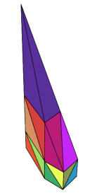
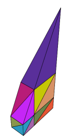
Figure 4. A triangulation of ${{\text{\hskip 0.85355pt\bf{C}}}}_{3}$ from two different angles.

4. Another subdivision of the Cayley polytope

The triangulation of the Cayley polytope described in the previous section proves Braun’s Conjecture by dividing the Cayley polytope into $(n+1)^{n-1}$ simplices. In this section we show how to subdivide the Cayley polytope into a much smaller number, $\operatorname{Cat}(n)$, of polytopes, each a direct product of orthoschemes. Potentially of independent interest, this constructions paves a way to prove Theorem 3.2.

Start by erasing all labels (but not the coordinates) from the labeled tree $\Phi(G)$, to make it into a plane tree $\Psi(G)$. For each node $v$ of a plane tree $T$ with successors with coordinates $x_{i}/2^{j},x_{i+1}/2^{j+1},\ldots,x_{i+k-1}/2^{j+k-1}$, take inequalities

$$1\hskip 1.70709pt\leq\hskip 1.70709ptx_{i+k-1}/2^{j+k-1}\hskip 1.70709pt\leq\hskip 1.70709pt\ldots\hskip 1.70709pt\leq x_{i+1}/2^{j+1}\hskip 1.70709pt\leq x_{i}/2^{j}\hskip 1.70709pt\leq 2\hskip 0.85355pt.$$

Equivalently, take inequalities

$$\begin{array}[]{lclcl}2^{j}&\!\!\!\leq\!\!&x_{i}&\!\!\!\leq\!\!&2^{j+1}\\ 2^{j+1}&\!\!\!\leq\!\!&x_{i+1}&\!\!\!\leq\!\!&2x_{i}\\ &&\vdots&&\\ 2^{j+k-1}&\!\!\!\leq\!\!&x_{i+k-1}&\!\!\!\leq\!\!&2x_{i+k-2}.\end{array}$$

Denote the resulting polytope ${{\text{\hskip 0.85355pt\bf{D}}}}_{T}$ (see Example 10.3).

Theorem 4.1

For every plane tree $T$ on $n+1$ nodes, the set ${{\text{\hskip 0.85355pt\bf{D}}}}_{T}$ is a bounded polytope, and

$$n!\hskip 0.85355pt{\text{\rm vol}}{{\text{\hskip 0.85355pt\bf{D}}}}_{T}\hskip 1.70709pt=\hskip 1.70709pt|\{G\in\mathcal{C}_{n+1}\,\,\mbox{{s.t.}}\ \Psi(G)=T\}|\hskip 1.70709pt=\hskip 1.70709pt2^{\binom{n+1}{2}-\sum_{i=1}^{n+1}id_{i}}\binom{n}{d_{1},d_{2},\ldots},$$

where $(d_{1},\ldots,d_{n+1})$ is the degree sequence of $T$. Furthermore, polytopes ${{\text{\hskip 0.85355pt\bf{D}}}}_{T}$ form a subdivision of the Cayley polytope ${{\text{\hskip 0.85355pt\bf{C}}}}_{n}$. In particular,

$$n!\hskip 0.85355pt{\text{\rm vol}}{{\text{\hskip 0.85355pt\bf{C}}}}_{n}\hskip 1.70709pt=\hskip 1.70709pt|\{G\in\mathcal{C}_{n+1}\}|\hskip 1.70709pt=\hskip 1.70709ptC_{n+1}.$$

Figure 5 shows two views of the resulting subdivision of ${{\text{\hskip 0.85355pt\bf{C}}}}_{3}$.

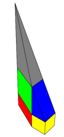
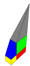
Figure 5. A subdivision of ${{\text{\hskip 0.85355pt\bf{C}}}}_{3}$ from two different angles.

5. The Gayley polytope

In this section we introduce the Gayley polytope ${{\text{\hskip 0.85355pt\bf{G}}}}_{n}$ which contains the Cayley polytope ${{\text{\hskip 0.85355pt\bf{C}}}}_{n}$ and whose volume corresponds to all labeled graphs, not just connected graphs.

Denote by $\mathcal{G}_{n}$ the set of labeled graphs on $n$ nodes. Obviously, $\mathcal{C}_{n}\subset\mathcal{G}_{n}$ and $|\mathcal{G}_{n}|=2^{\binom{n}{2}}$. Replace the $1$’s by $0$’s on the left-hand side of the inequalities defining the Cayley polytope; namely, define

$${{\text{\hskip 0.85355pt\bf{G}}}}_{n}=\{(x_{1},\ldots,x_{n})\colon 0\leq x_{1}\leq 2,0\leq x_{i}\leq 2\hskip 0.85355ptx_{i-1}\mbox{ for }i=2,\ldots,n\}$$

Note that ${{\text{\hskip 0.85355pt\bf{G}}}}_{n}$ is a Schläfli orthoscheme, ${{\text{\hskip 0.85355pt\bf{G}}}}_{n}={{\text{\hskip 0.85355pt\bf{O}}}}(2,4,\ldots,2^{n})$, and has volume $2^{\binom{n+1}{2}}/n!$. In other words,

$$n!\hskip 0.85355pt{\text{\rm vol}}{{\text{\hskip 0.85355pt\bf{G}}}}_{n}\hskip 1.70709pt=\hskip 1.70709pt|\{G\in\mathcal{G}_{n+1}\}|\hskip 0.85355pt.$$

Extending the construction in Section 3, we give an explicit triangulation of ${{\text{\hskip 0.85355pt\bf{G}}}}_{n}$ with simplices corresponding to labeled forests on $(n+1)$ nodes. This triangulation will prove useful later.

Start with an arbitrary graph $G$ on $n+1$ nodes. Order the components so that the maximal labels in the components are decreasing. Perform the NFS on each component of $G$ (see Section 2). The result is a labeled forest on $n+1$ nodes, we denote it by $\Phi(G)=F$. If $v$ has the maximal label in its component and there are $l$ nodes in previous components, choose the coordinate of $v$ to be $x_{l}$. In other words, $l$ is the position of the node in NFS. In particular, the coordinate of the node with label $n+1$ is $x_{0}$, which we set equal to $1$. Every other node $v$ has a coordinate of the form $x_{i}/2^{j}-x_{l}$, where $i$ is its position in NFS, $j$ is the number of cane paths in $F$ starting in $v$, and $l$ is the maximal label in the component of $v$. Denote the coordinate of the node with label $k$ in a forest $F$ by $c(k,F)$.

Define $\alpha(F)=\sum_{k}j_{k}$, where the sum is over nodes that do not have maximal labels in their components, and the coordinate of the node $k$ is $x_{i_{k}}/2^{j_{k}}-x_{l_{k}}$. By Lemma 3.1, $j_{k}$ is the number of cane paths starting in the node, and $\alpha(F)$ is the number of cane paths in the forest $F$.

Now arrange the coordinates of the nodes $1,\ldots,n+1$ according to the labels. More precisely, define

$${{\text{\hskip 0.85355pt\bf{S}}}}_{F}=\{(x_{1},\ldots,x_{n})\colon 0\leq c(1,F)\leq c(2,F)\leq\ldots\leq c(n+1,F)=1\}.$$

See Example 10.4.

The two definitions of ${{\text{\hskip 0.85355pt\bf{S}}}}_{T}$ for a tree coincide. Indeed, all the nodes except the one with label $n+1$ have coordinates of the form $x_{i}/2^{j}-1$, and adding $1$ to all the inequalities from the new definition of ${{\text{\hskip 0.85355pt\bf{S}}}}_{T}$ gets the inequalities in the first definition.

Theorem 5.1

For every labeled forest $F$ on $n+1$ nodes, the set ${{\text{\hskip 0.85355pt\bf{S}}}}_{F}$ is a simplex (but not in general an orthoscheme), and

$$n!\hskip 0.85355pt{\text{\rm vol}}{{\text{\hskip 0.85355pt\bf{S}}}}_{F}\hskip 1.70709pt=\hskip 1.70709pt|\{G\in\mathcal{G}_{n+1}\,\,\mbox{{s.t.}}\ \Phi(G)=F\}|\hskip 1.70709pt=\hskip 1.70709pt2^{\alpha(F)}\hskip 0.85355pt.$$

Furthermore, simplices ${{\text{\hskip 0.85355pt\bf{S}}}}_{F}$ triangulate the Gayley polytope ${{\text{\hskip 0.85355pt\bf{G}}}}_{n}$. In particular,

$$n!\hskip 0.85355pt{\text{\rm vol}}{{\text{\hskip 0.85355pt\bf{G}}}}_{n}\hskip 1.70709pt=\hskip 1.70709pt|\{G\in\mathcal{G}_{n+1}\}|\hskip 1.70709pt=\hskip 1.70709pt2^{\binom{n+1}{2}}\hskip 0.85355pt.$$

Although we already have a simple closed formula for the volume of Gayley polytopes, this result is a stepping stone towards our studies of Tutte polytopes (see below). The proof of the theorem is given in Section 11, and follows the same pattern as the proof of Theorem 3.2.

By analogy with Cayley polytopes, let us show that Gayley polytope can also be subdivided into a smaller number, $\operatorname{Cat}(n+1)$, of polytopes. Given $\mathbf{P}\subset{\mathbb{R}}^{n}$, define by

$$a\mathbf{P}=\{(ax_{1},\ldots,ax_{n})\colon(x_{1},\ldots,x_{n})\in\mathbf{P}\}\subset{\mathbb{R}}^{n}$$

the dilation of $\mathbf{P}$ by $a\in{\mathbb{R}}$, and by

$$\operatorname{Cone}(\mathbf{P})=\{(x_{0},x_{1},\ldots,x_{n})\colon 0\leq x_{0}\leq 1,(x_{1},\ldots,x_{n})\in x_{0}\mathbf{P}\}\subset{\mathbb{R}}^{n+1}.$$

the cone with apex $0$ and base $\{1\}\times\mathbf{P}$.

For an arbitrary graph $G$ on $n+1$ nodes, find the corresponding labeled forest $\Phi(G)$ and delete the labels to get a plane forest $\Psi(G)$ on $n+1$ nodes. For a plane forest $F$ on $n+1$ with components (plane trees) $T_{1},T_{2},T_{3},\ldots$, define

$${{\text{\hskip 0.85355pt\bf{D}}}}_{F}\hskip 1.70709pt=\hskip 1.70709pt{{\text{\hskip 0.85355pt\bf{D}}}}_{T_{1}}\times\operatorname{Cone}({{\text{\hskip 0.85355pt\bf{D}}}}_{T_{2}}\times\operatorname{Cone}({{\text{\hskip 0.85355pt\bf{D}}}}_{T_{3}}\times\cdots)).$$

Proposition 5.2

Take a plane forest $F$. For a node $w$ that is a root of its component, define coordinate $c(w,F)=x_{l}$, where $l$ is its position in NFS (equivalently, the components to the left have $l$ nodes total). For a node $v\neq w$ in the same component, define $c(v,F)=x_{i}/2^{j}-x_{l}$, where $i$ is its position in NFS and $j$ is the number of cane paths in $F$ starting in $v$.  For each node with successors $v_{1},\ldots,v_{k}$ (from left to right), take inequalities

$$0\leq c(v_{1},F)\leq\ldots c(v_{k},F)\leq c(w,F).$$

Furthermore, if $w_{1},\ldots,w_{m}$ are the roots of $F$ (from left to right), take inequalities

$$0\leq c(w_{m},F)\leq\ldots\leq c(w_{1},F)=1.$$

The resulting polytope is precisely ${{\text{\hskip 0.85355pt\bf{D}}}}_{F}$.

See Example 10.5. We need this proposition for the following theorem, aimed towards generalizations in the next sections.

Theorem 5.3

For every plane forest $F$ on $n+1$ nodes, the set ${{\text{\hskip 0.85355pt\bf{D}}}}_{F}$ is a bounded polytope, and

$$n!\hskip 0.85355pt{\text{\rm vol}}{{\text{\hskip 0.85355pt\bf{D}}}}_{F}\hskip 1.70709pt=\hskip 1.70709pt\left|\{G\in\mathcal{G}_{n+1}\,\mbox{{s.t.}}\ \Psi(G)=F\}\right|\hskip 1.70709pt=\hskip 1.70709pt\frac{\binom{n}{d_{1},d_{2},\ldots}}{\prod_{j=2}^{m}(a_{j}+\ldots+a_{m})}\cdot 2^{\binom{n+2-m}{2}-\sum_{i=1}^{n+1-m}id_{i}}\hskip 0.85355pt,$$

where $(d_{1},\ldots,d_{n+1-m})$ is the reduced degree sequence of $F$. Furthermore, polytopes ${{\text{\hskip 0.85355pt\bf{D}}}}_{F}$ form a subdivision of the Gayley polytope ${{\text{\hskip 0.85355pt\bf{G}}}}_{n}$. In particular,

$$n!\hskip 0.85355pt{\text{\rm vol}}{{\text{\hskip 0.85355pt\bf{G}}}}_{n}\hskip 1.70709pt=\hskip 1.70709pt\left|\{G\in\mathcal{G}_{n+1}\}\right|\hskip 1.70709pt=\hskip 1.70709pt2^{\binom{n+1}{2}}.$$

6. $t$-Cayley and $t$-Gayley polytopes

The constructions from the previous sections are easily adapted to weighted generalizations. Our presentation, the order and even shape of the results mimic the sections on Cayley and Gayley polytopes. All proofs are moved to Section 11, as before.

For $t\geq 0$, define the $t$-Cayley polytope ${{\text{\hskip 0.85355pt\bf{C}}}}_{n}(t)$ and the $t$-Gayley polytope ${{\text{\hskip 0.85355pt\bf{G}}}}_{n}(t)$ by replacing all $2$’s in the definition by $1+t$. More precisely, define

$${{\text{\hskip 0.85355pt\bf{C}}}}_{n}(t)=\{(x_{1},\ldots,x_{n})\colon 1\leq x_{1}\leq 1+t,1\leq x_{i}\leq(1+t)x_{i-1}\mbox{ for }i=2,\ldots,n\}$$

and

$${{\text{\hskip 0.85355pt\bf{G}}}}_{n}(t)=\{(x_{1},\ldots,x_{n})\colon 0\leq x_{1}\leq 1+t,0\leq x_{i}\leq(1+t)x_{i-1}\mbox{ for }i=2,\ldots,n\}.$$

We can triangulate the polytopes ${{\text{\hskip 0.85355pt\bf{C}}}}_{n}(t)$ and ${{\text{\hskip 0.85355pt\bf{G}}}}_{n}(t)$ (or subdivide them into larger polytopes like in Sections 4 and 5) in a very similar fashion as ${{\text{\hskip 0.85355pt\bf{C}}}}_{n}$ and ${{\text{\hskip 0.85355pt\bf{G}}}}_{n}$. For a labeled tree $T$ on $n+1$ nodes, attach a coordinate of the form $x_{i}/(1+t)^{j}$ to each node $v$ of $T$, where $i$ is the position of $v$ in NFS, and $j$ is the number of cane paths starting in $v$. Arrange the coordinates of the nodes according to the labels. More precisely, define

$${{\text{\hskip 0.85355pt\bf{S}}}}_{T}(t)=\{(x_{1},\ldots,x_{n})\colon 1\leq x_{i_{1}}/(1+t)^{j_{1}}\leq x_{i_{2}}/(1+t)^{j_{2}}\leq\ldots\leq x_{i_{n}}/(1+t)^{j_{n}}\leq 1+t\},$$

where the coordinate of the node with label $k$ is $x_{i_{k}}/(1+t)^{j_{k}}$. Note that the simplices ${{\text{\hskip 0.85355pt\bf{S}}}}_{T}(t)$ are also orthoschemes (see Example 10.6).

Theorem 6.1

For every labeled tree $T$ on $n+1$ nodes, the set ${{\text{\hskip 0.85355pt\bf{S}}}}_{T}(t)$ is a simplex, and

$$n!\hskip 0.85355pt{\text{\rm vol}}{{\text{\hskip 0.85355pt\bf{S}}}}_{T}(t)\,=\,\sum_{G\in\mathcal{C}_{n+1},\,\Phi(G)=T}t^{|E(G)|}\,=\,t^{n}(1+t)^{\alpha(T)}\hskip 0.85355pt.$$

Furthermore, simplices ${{\text{\hskip 0.85355pt\bf{S}}}}_{T}(t)$ triangulate the $t$-Cayley polytope ${{\text{\hskip 0.85355pt\bf{C}}}}_{n}(t)$. In particular,

$$n!\hskip 0.85355pt{\text{\rm vol}}{{\text{\hskip 0.85355pt\bf{C}}}}_{n}(t)\,=\,\sum_{G\in\mathcal{C}_{n+1}}t^{|E(G)|}\hskip 0.85355pt.$$

A similar construction works for the other subdivision. As in the non-weighted case, erase all labels from the labeled tree $\Phi(G)$ to make it into a plane tree $\Psi(G)$. For each node $v$ with successors with coordinates $x_{i}/(1+t)^{j},x_{i+1}/(1+t)^{j+1},\ldots,x_{i+k-1}/(1+t)^{j+k-1}$, take inequalities

$$1\leq x_{i+k-1}/(1+t)^{j+k-1}\leq\ldots\leq x_{i+1}/(1+t)^{j+1}\leq x_{i}/(1+t)^{j}\leq 1+t.$$

Denote the resulting polytope $\mathbf{D}_{T}(t)$ (see Example 10.7).

Theorem 6.2

For every plane tree $T$ on $n+1$ nodes, the set ${{\text{\hskip 0.85355pt\bf{D}}}}_{T}(t)$ is a bounded polytope, and

$$n!\hskip 0.85355pt{\text{\rm vol}}{{\text{\hskip 0.85355pt\bf{D}}}}_{T}(t)\hskip 1.70709pt=\hskip 1.70709pt\sum_{G\in\mathcal{G}_{n+1}\hskip 0.85355pt,\ \Psi(G)=T}\hskip 0.85355ptt^{|E(G)|}\hskip 1.70709pt=\hskip 1.70709ptt^{n}(1+t)^{\binom{n+1}{2}-\sum_{i=1}^{n+1}id_{i}}\cdot\binom{n}{d_{1},d_{2},\ldots},$$

where $(d_{1},\ldots,d_{n+1})$ is the degree sequence of $T$. Furthermore, polytopes ${{\text{\hskip 0.85355pt\bf{D}}}}_{T}(t)$ form a subdivision of the Cayley polytope ${{\text{\hskip 0.85355pt\bf{C}}}}_{n}(t)$. In particular,

$$n!\hskip 0.85355pt{\text{\rm vol}}{{\text{\hskip 0.85355pt\bf{C}}}}_{n}(t)\hskip 1.70709pt=\hskip 1.70709pt\sum_{G\in\mathcal{G}_{n+1}}\hskip 0.85355ptt^{|E(G)|}\hskip 0.85355pt.$$

Let us give a triangulation of the $t$-Gayley polytope. Take a labeled forest $F$ on $n+1$ nodes. If $v$ has the maximal label in its component and there are $i$ nodes in previous components, choose the coordinate of $v$ to be $tx_{i}$. In particular, the coordinate of the node with label $n+1$ is $tx_{0}=t$. Every other node $v$ has a coordinate of the form $x_{i}/(1+t)^{j}-x_{l}$, where $i$ is the position of $v$ in NFS, $j$ is the number of cane paths in $F$ starting in $v$, and $l$ is the maximal label in the component of $v$. Denote the coordinate of the node with label $k$ in a forest $F$ by $c(k,F;t)$.

Now arrange the coordinates of the nodes according to the labels. More precisely, define

$${{\text{\hskip 0.85355pt\bf{S}}}}_{F}(t)=\{(x_{1},\ldots,x_{n})\colon 0\leq c(1,F;t)\leq c(2,F;t)\leq\ldots\leq c(n+1,F;t)=t\}.$$

See Example 10.8.

Theorem 6.3

For every labeled forest $F$ on $n+1$ nodes, the set ${{\text{\hskip 0.85355pt\bf{S}}}}_{F}(t)$ is a simplex (but not in general an orthoscheme), and

$$n!\hskip 0.85355pt{\text{\rm vol}}{{\text{\hskip 0.85355pt\bf{S}}}}_{F}(t)\hskip 1.70709pt=\hskip 1.70709pt\sum_{G\in\mathcal{G}_{n+1}\hskip 0.85355pt,\ \Phi(G)=F}t^{|E(G)|}\hskip 1.70709pt=\hskip 1.70709ptt^{|E(F)|}(1+t)^{\alpha(F)}.$$

Furthermore, simplices ${{\text{\hskip 0.85355pt\bf{S}}}}_{F}(t)$ triangulate the $t$-Gayley polytope ${{\text{\hskip 0.85355pt\bf{G}}}}_{n}(t)$. In particular,

$$n!\hskip 0.85355pt{\text{\rm vol}}{{\text{\hskip 0.85355pt\bf{G}}}}_{n}(t)\hskip 1.70709pt=\hskip 1.70709pt\sum_{G\in\mathcal{G}_{n+1}}t^{|E(G)|}\hskip 1.70709pt=\hskip 1.70709pt(1+t)^{\binom{n+1}{2}}.$$

We can also subdivide the $t$-Gayley polytope into a smaller number, $\operatorname{Cat}(n+1)$, of polytopes. Recall that for an arbitrary graph $G$ on $n+1$ nodes, we have found the corresponding labeled forest $\Phi(G)$ and deleted the labels to get a plane forest $\Psi(G)$ on $n+1$ nodes. For a plane forest $F$ on $n+1$ nodes with components (plane trees) $T_{1},\ldots,T_{k}$, define

$${{\text{\hskip 0.85355pt\bf{D}}}}_{F}(t)={{\text{\hskip 0.85355pt\bf{D}}}}_{T_{1}}(t)\times\operatorname{Cone}({{\text{\hskip 0.85355pt\bf{D}}}}_{T_{2}}(t)\times\operatorname{Cone}({{\text{\hskip 0.85355pt\bf{D}}}}_{T_{3}}(t)\times\cdots)).$$

Proposition 6.4

Take a plane forest $F$. For a node $w$ that is a root of its component, define coordinate $c(w,F;t)=tx_{l}$, where $l$ is its position in NFS (equivalently, the components to the left have $l$ nodes total). For a node $v\neq w$ in the same component, define $c(v,F;t)=x_{i}/(1+t)^{j}-x_{l}$, where $i$ is its position in NFS and $j$ is the number of cane paths in $F$ starting in $v$.  For each node with successors $v_{1},\ldots,v_{k}$ (from left to right), take inequalities

$$0\leq c(v_{1},F;t)\leq\ldots c(v_{k},F;t)\leq c(w,F;t).$$

Furthermore, if $w_{1},\ldots,w_{m}$ are the roots of $F$ (from left to right), take inequalities

$$0\leq c(w_{m},F;t)\leq\ldots\leq c(w_{1},F;t)=t.$$

The resulting polytope is precisely ${{\text{\hskip 0.85355pt\bf{D}}}}_{F}(t)$.

See Example 10.9.

Theorem 6.5

For every plane forest $F$ on $n+1$ nodes, the set ${{\text{\hskip 0.85355pt\bf{D}}}}_{F}(t)$ is a bounded polytope, and

$$n!\hskip 0.85355pt{\text{\rm vol}}{{\text{\hskip 0.85355pt\bf{D}}}}_{F}(t)\hskip 1.70709pt=\!\!\!\!\!\sum_{G\in\mathcal{G}_{n+1},\Psi(G)=F}\!\!\!\!\!\!\!t^{|E(G)|}=\hskip 1.70709pt\frac{\binom{n}{d_{1},d_{2},\ldots}}{\prod_{j=2}^{m}(a_{j}+\ldots+a_{m})}t^{\sum_{i=1}^{n+1-m}d_{i}}(1+t)^{\binom{n+2-m}{2}-\sum_{i=1}^{n+1-m}id_{i}}$$

where $(d_{1},\ldots,d_{n+1-m})$ is the reduced degree sequence of $F$. Furthermore, polytopes ${{\text{\hskip 0.85355pt\bf{D}}}}_{F}(t)$ form a subdivision of the $t$-Gayley polytope ${{\text{\hskip 0.85355pt\bf{G}}}}_{n}(t)$. In particular,

$$n!\hskip 0.85355pt{\text{\rm vol}}{{\text{\hskip 0.85355pt\bf{G}}}}_{n}(t)\hskip 1.70709pt=\hskip 1.70709pt\sum_{G\in\mathcal{G}_{n+1}}t^{|E(G)|}\hskip 1.70709pt=\hskip 1.70709pt(1+t)^{\binom{n+1}{2}}.$$

7. The Tutte polytope

Recall that we defined the Tutte polytope by inequalities

$$qx_{i}\leq q(1+t)x_{i-1}-t(1-q)(1-x_{j-1}),$$

where $1\leq j\leq i\leq n$ and $x_{0}=1$. Here $0<q\leq 1$ and $t>0$. We have already established that it specializes to:

• the Cayley polytope for $q=0$, $t=1$,

• the Gayley polytope for $q=1$, $t=1$,

• the $t$-Cayley polytope for $q=0$,

• the $t$-Gayley polytope for $q=1$.

In this section, we construct a triangulation and a subdivision of this polytope that prove Theorem 1.3. Recall that in the previous section, we were given a labeled forest $F$ and we attached a coordinate of the form $c(l,F;t)=tx_{l}$ to every root of the forest (where $x_{0}=1$), and $c(i,F;t)=x_{i}/(1+t)^{j}-x_{l}$ to every non-root node. Now the role of the former will be played by

$$c(l,F;q,t)=t(x_{l}-1+q)\hskip 0.85355pt,$$

and of the latter by

$$c(i,F;q,t)=\frac{qx_{i}-(1-q)(1-x_{l})}{(1+t)^{j}}-(x_{l}-1+q)\hskip 0.85355pt.$$

Note that $c(i,F;1,t)=c(i,F;t)$ for all $i$. Define

$${{\text{\hskip 0.85355pt\bf{S}}}}_{F}(q,t)=\{(x_{1},\ldots,x_{n})\colon 0\leq c(1,F;q,t)\leq c(2,F;q,t)\leq\ldots\leq c(n+1,F;q,t)=qt\}\hskip 0.85355pt.$$

Theorem 7.1

For every labeled forest $F$ on $n+1$ nodes, the set ${{\text{\hskip 0.85355pt\bf{S}}}}_{F}(q,t)$ is a simplex, and

$$n!\hskip 0.85355pt{\text{\rm vol}}{{\text{\hskip 0.85355pt\bf{S}}}}_{F}(q,t)\hskip 1.70709pt=\hskip 1.70709pt\sum_{G\in\mathcal{G}_{n+1}\hskip 0.85355pt,\ \Phi(G)=F}q^{k(G)-1}t^{|E(G)|}=q^{k(F)-1}t^{|E(F)|}(1+t)^{\alpha(F)}.$$

Furthermore, simplices ${{\text{\hskip 0.85355pt\bf{S}}}}_{F}(q,t)$ triangulate the Tutte polytope ${{\text{\hskip 0.85355pt\bf{T}}}}_{n}(q,t)$. In particular,

$$n!\hskip 0.85355pt{\text{\rm vol}}{{\text{\hskip 0.85355pt\bf{T}}}}_{n}(q,t)\hskip 1.70709pt=\hskip 1.70709pt\sum_{G\in\mathcal{G}_{n+1}}q^{k(G)-1}t^{|E(G)|}.$$

In other words,

$$(\heartsuit)\ \ \ n!\hskip 0.85355pt{\text{\rm vol}}{{\text{\hskip 0.85355pt\bf{T}}}}_{n}(q,t)\hskip 1.70709pt=\hskip 1.70709pt{\text{\rm Z}}_{K_{n+1}}(q,t).$$

This is a key result in this paper which implies Main Theorem (Theorem 3.2). The proof is based on an extension of the previous results for $t$-Cayley and $t$-Gayley polytopes. Although the technical details are quite a bit trickier in this case, the structure of the proof follows the same pattern as before.

For $q>0$ and $\mathbf{P}\subset{\mathbb{R}}^{n}$, define

$$\operatorname{Cone}_{q}(\mathbf{P})=\{(x_{0},x_{1},\ldots,x_{n})\colon 1-q\leq x_{0}\leq 1,q(x_{1},\ldots,x_{n})\in(x_{0}-1+q)\mathbf{P}+(1-q)(1-x_{0})\}.$$

the cone with apex $(1-q,\ldots,1-q)$ and base $\{1\}\times\mathbf{P}$.

For a plane forest $F$ on $n+1$ with components (plane trees) $T_{1},T_{2},T_{3},\ldots$, define

$$D_{F}(q,t)=\mathbf{D}_{T_{1}}(t)\times\operatorname{Cone}_{q}(\mathbf{D}_{T_{2}}(t)\times\operatorname{Cone}_{q}(\mathbf{D}_{T_{3}}(t)\times\cdots)).$$

Proposition 7.2

Take a plane forest $F$. For a node $w$ that is a root of its component, define coordinate $c(w,F;q,t)=t(x_{l}-1+q)$, where $l$ is its position in NFS (equivalently, the components to the left have $l$ nodes total). For a node $v\neq w$ in the same component, define

$$c(v,F;q,t)\hskip 1.70709pt=\hskip 1.70709pt\frac{qx_{i}-(1-q)(1-x_{l})}{(1+t)^{j}}\hskip 1.70709pt-\hskip 1.70709pt(x_{l}-1+q)\hskip 1.70709pt,$$

where $i$ is its position in NFS and $j$ is the number of cane paths in $F$ starting in $v$.  For each node with successors $v_{1},\ldots,v_{k}$ (from left to right), take inequalities

$$0\leq c(v_{1},F;q,t)\leq\ldots\leq c(v_{k},F;q,t)\leq c(w,F;q,t)\hskip 0.85355pt.$$

Furthermore, if $w_{1},\ldots,w_{m}$ are the roots of $F$ (from left to right), take inequalities

$$0\leq c(w_{m},F;q,t)\leq\ldots\leq c(w_{1},F;q,t)=tq\hskip 0.85355pt.$$

The resulting polytope is precisely ${{\text{\hskip 0.85355pt\bf{D}}}}_{F}(q,t)$.

This proposition is used to prove the following result of independent interest, a theorem which is in turn used to derive Theorem 7.1 in Section 11.

Theorem 7.3

For every plane forest $F$ on $n+1$ nodes, the set ${{\text{\hskip 0.85355pt\bf{D}}}}_{F}(q,t)$ is a bounded polytope, and

$$n!\hskip 0.85355pt{\text{\rm vol}}{{\text{\hskip 0.85355pt\bf{D}}}}_{F}(q,t)\hskip 1.70709pt=\hskip 1.70709pt\sum_{G\in\mathcal{G}_{n+1}\hskip 0.85355pt,\ \Psi(G)=F}q^{k(G)-1}t^{|E(G)|}\hskip 1.70709pt=$$

$$=\hskip 1.70709pt\frac{\binom{n}{d_{1},d_{2},\ldots}}{\prod_{j=2}^{m}(a_{j}+\ldots+a_{m})}\,q^{k(F)-1}t^{\sum_{i=1}^{n+1-m}d_{i}}(1+t)^{\binom{n+2-m}{2}\hskip 0.85355pt-\hskip 0.85355pt\sum_{i=1}^{n+1-m}\hskip 0.85355pti\hskip 0.85355ptd_{i}}\hskip 1.70709pt,$$

where $(d_{1},\ldots,d_{n+1-m})$ is the reduced degree sequence of $F$. Furthermore, polytopes ${{\text{\hskip 0.85355pt\bf{D}}}}_{F}(q,t)$ form a subdivision of the Tutte polytope ${{\text{\hskip 0.85355pt\bf{T}}}}_{n}(q,t)$. In particular,

$$n!\hskip 0.85355pt{\text{\rm vol}}\mathbf{T}_{n}(t)\hskip 1.70709pt=\hskip 1.70709pt\sum_{G\in\mathcal{G}_{n+1}}q^{k(G)-1}t^{|E(G)|}\hskip 1.70709pt=\hskip 1.70709pt{\text{\rm Z}}_{K_{n+1}}(q,t)\hskip 0.85355pt.$$

8. Vertices

The inequalities defining the Tutte polytope, as well as the simplices in the triangulation, are quite complicated compared to the ones for $t$-Cayley and $t$-Gayley polytopes. In this section, we see that the vertices of all the polytopes involved are very simple.

The following propositions give the vertices of the simplices ${{\text{\hskip 0.85355pt\bf{S}}}}_{F}(t)$ for $F$ a labeled forest, and of the $t$-Cayley polytope.

Proposition 8.1

Pick $t>0$ and a labeled forest $F$ on $n+1$ nodes. The set of vertices of the simplex ${{\text{\hskip 0.85355pt\bf{S}}}}_{F}(t)$ is the set $V(F;t)=\{v_{p}(F;t),1\leq p\leq n+1\}$, where $v_{p}(F;t)=(x_{1},\ldots,x_{n})$ satisfies the following:

1. if the node $v$ is the $l$-th visited and its label $r$ is maximal in its component, then

   $$x_{l}=\left\{\begin{array}[]{ccl}1&:&p\leq r\\ 0&:&p>r\end{array}\right.$$

2. if the node $v$ is the $i$-th visited and its label $k$ is not $r$, the maximal label in its component, then

   $$x_{i}=\left\{\begin{array}[]{ccl}(1+t)^{j+1}&:&p\leq k\\ (1+t)^{j}&:&k<p\leq r\\ 0&:&p>r\end{array}\right.$$

   where $j$ is the number of cane paths in $F$ starting in $v$.

Proposition 8.2

For $t>0$, the set of vertices of ${{\text{\hskip 0.85355pt\bf{C}}}}_{n}(t)$ is the set

$$V_{n}(t)=\bigl{\{}(x_{1},\ldots,x_{n})\colon\hskip 1.70709ptx_{1}\in\{1,1+t\},\,x_{i}\in\{1,(1+t)\hskip 0.85355ptx_{i-1}\}\ \,\text{for}\ \hskip 1.70709pti=2,\ldots,n\bigr{\}}\hskip 0.85355pt.$$

Examples 10.10 and 10.11 illustrate these propositions. For a labeled forest $F$, let $V(F;q,t)$ be the set of points that we get if we replace the (trailing) $0$’s in the coordinates of the points in $V(F;t)$ by $1-q$ (see Example 10.12).

Proposition 8.3

For a labeled forest $F$ and $t>0$, $0<q\leq 1$, $V(F;q,t)$ is the set of vertices of ${{\text{\hskip 0.85355pt\bf{S}}}}_{F}(q,t)$.

Let $V_{n}(q,t)$ be the set $V_{n}(t)$ in which we replace the trailing $1$’s of each point by $1-q$ (see Example 10.13). We conclude with the main result of this section:

Theorem 8.4

For $t>0$ and $0\leq q<1$, $V_{n}(q,t)$ is the set of vertices of $\mathbf{T}_{n}(q,t)$. In particular, the Tutte polytope $\mathbf{T}_{n}(q,t)$ has $2^{n}$ vertices.

9. Application: a recursive formula

The results proved in this paper yield an interesting recursive formulas for the generating function for (or the number of) labeled connected graphs. Let

$$F_{n}(t)\hskip 1.70709pt=\hskip 1.70709pt\sum t^{|E(G)|}\hskip 1.70709pt=\hskip 1.70709ptt^{n-1}\hskip 0.85355pt\operatorname{Inv}_{n}(1+t)\hskip 0.85355pt,$$

where the sum is over labeled connected graphs on $n$ nodes.

Theorem 9.1

Define polynomials $r_{n}(t)$, $n\geq 0$, by

$$r_{0}(t)=1,\qquad r_{n}(t)=-\sum_{j=1}^{n}\binom{n}{j}(1+t)^{\binom{j}{2}}r_{n-j}(t).$$

Then

$$F_{n+1}(t)=\sum_{j=0}^{n}\binom{n}{j}(1+t)^{\binom{j+1}{2}}r_{n-j}(t).$$

Proof.

Define

$$I_{n}(x,t)=n!\int_{1}^{(1+t)x}dx_{1}\int_{1}^{(1+t)x_{1}}dx_{2}\int_{1}^{(1+t)x_{2}}dx_{3}\cdots\int_{1}^{(1+t)x_{n-1}}dx_{n}.$$

Clearly, we have

$$I_{n}(x,t)=n\int_{1}^{(1+t)x}I_{n-1}(x_{1},t)dx_{1}.$$

We claim that

$$I_{n}(x,t)=\sum_{j=0}^{n}\binom{n}{j}(1+t)^{\binom{j+1}{2}}r_{n-j}(t)x^{j},$$

where the polynomials $r_{j}(t)$ are defined in Theorem 9.1. Indeed, the statement is obviously true for $n=0$, and by induction,

$$I_{n}(x,t)=n\int_{1}^{(1+t)x}\left(\sum_{j=0}^{n-1}\binom{n-1}{j}(1+t)^{\binom{j+1}{2}}r_{n-1-j}(t)x_{1}^{j}\right)dx_{1}=$$

$$=n\sum_{j=0}^{n-1}\binom{n-1}{j}(1+t)^{\binom{j+1}{2}}r_{n-1-j}(t)\left(\frac{(1+t)^{j+1}}{j+1}x^{j+1}-\frac{1}{j+1}\right)=$$

$$=\sum_{j=1}^{n}\binom{n}{j}(1+t)^{k+1}r_{n-j}(t)x^{j}-\sum_{j=0}^{n-1}\binom{n}{j+1}(1+t)^{\binom{j+1}{2}}r_{n-1-j}(t),$$

which by definition of $r_{n}(t)$ equals

$$\sum_{j=0}^{n}\binom{n}{j}(1+t)^{\binom{j+1}{2}}r_{n-j}(t)x^{j}.$$

Theorem 9.1 follows by plugging in $x=1$ into the equation. ∎

10. Examples

Example 10.1

Let $G$ be the graph on the left-hand side of Figure 6. The neighbors-first search starts in node $12$ and visits the other nodes in order $11,10,6,8,7,9,3,1,4,2,5$. The resulting search tree $\Phi(G)$ is on the right-hand side of Figure 6. The edges of $G$ that are not in $\Phi(G)$ are dashed.

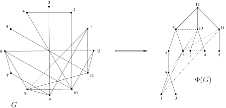
Figure 6. A connected graph and its NFS tree.

Example 10.2

For the tree $T$ drawn on the right-hand side of Figure 6, the coordinates of the nodes with labels $1,\ldots,11$ are shown in Figure 7. We have $\alpha(T)=21$.

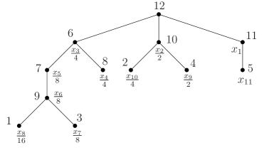
Figure 7. Coordinates in a tree.

The corresponding set ${{\text{\hskip 0.85355pt\bf{S}}}}_{T}$ is the set of points $(x_{1},\ldots,x_{11})$ satisfying

$$1\leq\frac{x_{8}}{16}\leq\frac{x_{10}}{4}\leq\frac{x_{7}}{8}\leq\frac{x_{9}}{2}\leq x_{11}\leq\frac{x_{3}}{4}\leq\frac{x_{5}}{8}\leq\frac{x_{4}}{4}\leq\frac{x_{6}}{8}\leq\frac{x_{2}}{2}\leq x_{1}\leq 2\hskip 0.85355pt.$$

Example 10.3

For the graph $G$ from the left-hand side of Figure 6, $\mathbf{D}_{\Psi(G)}(t)$ is

$$\left\{\begin{array}[]{llll}(x_{1},\ldots,x_{11})\colon&1\leq x_{1}\leq 2,&2\leq x_{2}\leq 2\hskip 0.85355ptx_{1},&4\leq x_{3}\leq 2\hskip 0.85355ptx_{2},\\ 4\leq x_{4}\leq 8,&8\leq x_{5}\leq 2\hskip 0.85355ptx_{4},&8\leq x_{6}\leq 16,&8\leq x_{7}\leq 16,\\ 16\leq x_{8}\leq 2\hskip 0.85355ptx_{7},&2\leq x_{9}\leq 4,&4\leq x_{10}\leq 2\hskip 0.85355ptx_{9},&1\leq x_{11}\leq 2\end{array}\right\}.$$

Example 10.4

Take $G$ to be the (disconnected) graph on the left-hand side of Figure 8. The search forest $F$ of the NFS is given on the right.

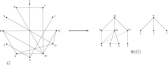
Figure 8. A disconnected graph and its NFS forest.

Figure 9 illustrates the coordinates we attach to the nodes of the forest $F$. The corresponding set ${{\text{\hskip 0.85355pt\bf{S}}}}_{F}$ is the set of points $(x_{1},\ldots,x_{11})$ satisfying

$$0\leq\frac{x_{11}}{4}-x_{8}\leq\frac{x_{6}}{4}-1\leq\frac{x_{10}}{2}-x_{8}\leq\frac{x_{5}}{2}-1\leq x_{7}-1\leq$$

$$\leq\frac{x_{3}}{4}-1\leq x_{9}-x_{8}\leq\frac{x_{4}}{4}-1\leq x_{8}\leq\frac{x_{2}}{2}-1\leq x_{1}-1\leq 1.$$

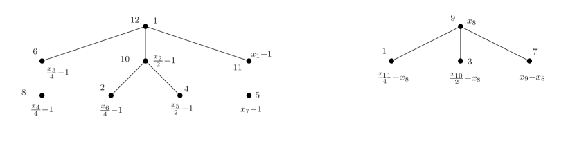
Figure 9. Coordinates in a forest.

Example 10.5

For the right component $T_{2}$ of the forest on the right-hand side of Figure 8,

$${{\text{\hskip 0.85355pt\bf{D}}}}_{T_{2}}\hskip 1.70709pt=\hskip 1.70709pt\{(x_{1},x_{2},x_{3})\colon 1\leq x_{1}\leq 2\hskip 0.85355pt,\hskip 1.70709pt2\leq x_{2}\leq 2\hskip 0.85355ptx_{1}\hskip 0.85355pt,\hskip 1.70709pt4\leq x_{3}\leq 2\hskip 0.85355ptx_{2}\},$$

so

$$\operatorname{Cone}({{\text{\hskip 0.85355pt\bf{D}}}}_{T_{2}})\hskip 1.70709pt=\hskip 1.70709pt\left\{(x_{0},x_{1},x_{2},x_{3})\colon 0\leq x_{0}\leq 1,\hskip 1.70709pt1\leq\frac{x_{1}}{x_{0}}\leq 2,\hskip 1.70709pt2\leq\frac{x_{2}}{x_{0}}\leq 2\hskip 0.85355pt\frac{x_{1}}{x_{0}},\hskip 1.70709pt4\leq\frac{x_{3}}{x_{0}}\leq 2\hskip 0.85355pt\frac{x_{2}}{x_{0}}\right\}.$$

For the graph $G$ from the left-hand side of Figure 8, $\mathbf{D}_{\Psi(G)}$ is

$$\left\{\begin{array}[]{llll}(x_{1},\ldots,x_{11})\colon&1\leq x_{1}\leq 2,&2\leq x_{2}\leq 2\hskip 0.85355ptx_{1},&4\leq x_{3}\leq 2\hskip 0.85355ptx_{2},\\ 4\leq x_{4}\leq 8,&2\leq x_{5}\leq 4,&4\leq x_{6}\leq 2\hskip 0.85355ptx_{5},&1\leq x_{7}\leq 2,\\ 0\leq x_{8}\leq 1,&x_{8}\leq x_{9}\leq 2\hskip 0.85355ptx_{8},&2\hskip 0.85355ptx_{8}\leq x_{10}\leq 2\hskip 0.85355ptx_{9},&4\hskip 0.85355ptx_{8}\leq x_{11}\leq 2\hskip 0.85355ptx_{10}\end{array}\right\}.$$

Example 10.6

For the graph $G$ on the left-hand side of Figure 6, $S_{\Phi(G)}(t)$ is the set of points $(x_{1},\ldots,x_{11})$ satisfying

$$1\leq\frac{x_{8}}{(1+t)^{4}}\leq\frac{x_{10}}{(1+t)^{2}}\leq\frac{x_{7}}{(1+t)^{3}}\leq\frac{x_{9}}{1+t}\leq x_{11}\leq\frac{x_{3}}{(1+t)^{2}}\leq$$

$$\leq\frac{x_{5}}{(1+t)^{3}}\leq\frac{x_{4}}{(1+t)^{2}}\leq\frac{x_{6}}{(1+t)^{3}}\leq\frac{x_{2}}{1+t}\leq x_{1}\leq 1+t.$$

Example 10.7

For the graph $G$ from the left-hand side of Figure 6, $\mathbf{D}_{\Psi(G)}(t)$ is

$$\left\{\begin{array}[]{lll}(x_{1},\ldots,x_{11})\colon&1\leq x_{1}\leq 1+t,&1+t\leq x_{2}\leq(1+t)\hskip 0.85355ptx_{1},\\ (1+t)^{2}\leq x_{3}\leq(1+t)\hskip 0.85355ptx_{2},&(1+t)^{2}\leq x_{4}\leq(1+t)^{3},&(1+t)^{3}\leq x_{5}\leq(1+t)\hskip 0.85355ptx_{4},\\ (1+t)^{3}\leq x_{6}\leq(1+t)^{4},&(1+t)^{3}\leq x_{7}\leq(1+t)^{4},&(1+t)^{4}\leq x_{8}\leq(1+t)\hskip 0.85355ptx_{7},\\ 1+t\leq x_{9}\leq(1+t)^{2},&(1+t)^{2}\leq x_{10}\leq(1+t)\hskip 0.85355ptx_{9},&1\leq x_{11}\leq 1+t\end{array}\right\}.$$

Example 10.8

Take $G$ to be the graph on the left-hand side of Figure 8. Figure 10 illustrates the coordinates we attach to the nodes of the corresponding forest $F$. The corresponding set ${{\text{\hskip 0.85355pt\bf{S}}}}_{F}(t)$ is the set of points $(x_{1},\ldots,x_{11})$ satisfying

$$0\leq\frac{x_{11}}{(1+t)^{2}}-x_{8}\leq\frac{x_{6}}{(1+t)^{2}}-1\leq\frac{x_{10}}{1+t}-x_{8}\leq\frac{x_{5}}{1+t}-1\leq x_{7}-1\leq$$

$$\leq\frac{x_{3}}{(1+t)^{2}}-1\leq x_{9}-x_{8}\leq\frac{x_{4}}{(1+t)^{2}}-1\leq tx_{8}\leq\frac{x_{2}}{1+t}-1\leq x_{1}-1\leq t.$$

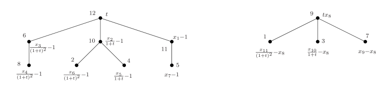
Figure 10. Coordinates in a forest (the $t$-Gayley case).

Example 10.9

For the graph $G$ from the left-hand side of Figure 8, $\mathbf{D}_{\Psi(G)}(t)$ is

$$\left\{\begin{array}[]{lll}(x_{1},\ldots,x_{11})\colon&1\leq x_{1}\leq 1+t,&1+t\leq x_{2}\leq(1+t)\hskip 0.85355ptx_{1},\\ (1+t)^{2}\leq x_{3}\leq(1+t)\hskip 0.85355ptx_{2},&(1+t)^{2}\leq x_{4}\leq(1+t)^{3},&1+t\leq x_{5}\leq(1+t)^{2},\\ (1+t)^{2}\leq x_{6}\leq(1+t)\hskip 0.85355ptx_{5},&1\leq x_{7}\leq 1+t,&0\leq x_{8}\leq 1,\\ x_{8}\leq x_{9}\leq(1+t)\hskip 0.85355ptx_{8},&(1+t)x_{8}\leq x_{10}\leq(1+t)\hskip 0.85355ptx_{9},&(1+t)^{2}\hskip 0.85355ptx_{8}\leq x_{11}\leq(1+t)\hskip 0.85355ptx_{10}\end{array}\right\}.$$

Example 10.10

The coordinates of the vertices of ${{\text{\hskip 0.85355pt\bf{S}}}}_{F}(t)$ for the forest from Figure 10 are given by lines in the following table:

$$\setcounter{MaxMatrixCols}{11}\begin{matrix}1+t&(1+t)^{2}&(1+t)^{3}&(1+t)^{3}&(1+t)^{2}&(1+t)^{3}&1+t&1&1+t&(1+t)^{2}&(1+t)^{3}\\ 1+t&(1+t)^{2}&(1+t)^{3}&(1+t)^{3}&(1+t)^{2}&(1+t)^{3}&1+t&1&1+t&(1+t)^{2}&(1+t)^{2}\\ 1+t&(1+t)^{2}&(1+t)^{3}&(1+t)^{3}&(1+t)^{2}&(1+t)^{2}&1+t&1&1+t&(1+t)^{2}&(1+t)^{2}\\ 1+t&(1+t)^{2}&(1+t)^{3}&(1+t)^{3}&(1+t)^{2}&(1+t)^{2}&1+t&1&1+t&1+t&(1+t)^{2}\\ 1+t&(1+t)^{2}&(1+t)^{3}&(1+t)^{3}&1+t&(1+t)^{2}&1+t&1&1+t&1+t&(1+t)^{2}\\ 1+t&(1+t)^{2}&(1+t)^{3}&(1+t)^{3}&1+t&(1+t)^{2}&1&1&1+t&1+t&(1+t)^{2}\\ 1+t&(1+t)^{2}&(1+t)^{2}&(1+t)^{3}&1+t&(1+t)^{2}&1&1&1+t&1+t&(1+t)^{2}\\ 1+t&(1+t)^{2}&(1+t)^{2}&(1+t)^{3}&1+t&(1+t)^{2}&1&1&1&1+t&(1+t)^{2}\\ 1+t&(1+t)^{2}&(1+t)^{2}&(1+t)^{2}&1+t&(1+t)^{2}&1&1&1&1+t&(1+t)^{2}\\ 1+t&(1+t)^{2}&(1+t)^{2}&(1+t)^{2}&1+t&(1+t)^{2}&1&0&0&0&0\\ 1+t&1+t&(1+t)^{2}&(1+t)^{2}&1+t&(1+t)^{2}&1&0&0&0&0\\ 1&1+t&(1+t)^{2}&(1+t)^{2}&1+t&(1+t)^{2}&1&0&0&0&0\end{matrix}$$

Example 10.11

The coordinates of the vertices of ${{\text{\hskip 0.85355pt\bf{C}}}}_{3}(t)$ are given by lines in the following table:

$$\begin{matrix}1+t&(1+t)^{2}&(1+t)^{3}\\ 1+t&(1+t)^{2}&1\\ 1+t&1&1+t\\ 1+t&1&1\\ 1&1+t&(1+t)^{2}\\ 1&1+t&1\\ 1&1&1+t\\ 1&1&1\end{matrix}$$

Example 10.12

The coordinates of the vertices of ${{\text{\hskip 0.85355pt\bf{S}}}}_{F}(q,t)$ for the forest from Figure 10 are given by lines in the following table:

$$\setcounter{MaxMatrixCols}{11}\begin{matrix}1+t&\!\!\>(1+t)^{2}&\!\!\>(1+t)^{3}&\!\!\>(1+t)^{3}&\!\!\>(1+t)^{2}&\!\!\>(1+t)^{3}&\!\!\>1+t&\!\!\>1&\!\!\>1+t&\!\!\>(1+t)^{2}&\!\!\>(1+t)^{3}\\ 1+t&\!\!\>(1+t)^{2}&\!\!\>(1+t)^{3}&\!\!\>(1+t)^{3}&\!\!\>(1+t)^{2}&\!\!\>(1+t)^{3}&\!\!\>1+t&\!\!\>1&\!\!\>1+t&\!\!\>(1+t)^{2}&\!\!\>(1+t)^{2}\\ 1+t&\!\!\>(1+t)^{2}&\!\!\>(1+t)^{3}&\!\!\>(1+t)^{3}&\!\!\>(1+t)^{2}&\!\!\>(1+t)^{2}&\!\!\>1+t&\!\!\>1&\!\!\>1+t&\!\!\>(1+t)^{2}&\!\!\>(1+t)^{2}\\ 1+t&\!\!\>(1+t)^{2}&\!\!\>(1+t)^{3}&\!\!\>(1+t)^{3}&\!\!\>(1+t)^{2}&\!\!\>(1+t)^{2}&\!\!\>1+t&\!\!\>1&\!\!\>1+t&\!\!\>1+t&\!\!\>(1+t)^{2}\\ 1+t&\!\!\>(1+t)^{2}&\!\!\>(1+t)^{3}&\!\!\>(1+t)^{3}&\!\!\>1+t&\!\!\>(1+t)^{2}&\!\!\>1+t&\!\!\>1&\!\!\>1+t&\!\!\>1+t&\!\!\>(1+t)^{2}\\ 1+t&\!\!\>(1+t)^{2}&\!\!\>(1+t)^{3}&\!\!\>(1+t)^{3}&\!\!\>1+t&\!\!\>(1+t)^{2}&\!\!\>1&\!\!\>1&\!\!\>1+t&\!\!\>1+t&\!\!\>(1+t)^{2}\\ 1+t&\!\!\>(1+t)^{2}&\!\!\>(1+t)^{2}&\!\!\>(1+t)^{3}&\!\!\>1+t&\!\!\>(1+t)^{2}&\!\!\>1&\!\!\>1&\!\!\>1+t&\!\!\>1+t&\!\!\>(1+t)^{2}\\ 1+t&\!\!\>(1+t)^{2}&\!\!\>(1+t)^{2}&\!\!\>(1+t)^{3}&\!\!\>1+t&\!\!\>(1+t)^{2}&\!\!\>1&\!\!\>1&\!\!\>1&\!\!\>1+t&\!\!\>(1+t)^{2}\\ 1+t&\!\!\>(1+t)^{2}&\!\!\>(1+t)^{2}&\!\!\>(1+t)^{2}&\!\!\>1+t&\!\!\>(1+t)^{2}&\!\!\>1&\!\!\>1&\!\!\>1&\!\!\>1+t&\!\!\>(1+t)^{2}\\ 1+t&\!\!\>(1+t)^{2}&\!\!\>(1+t)^{2}&\!\!\>(1+t)^{2}&\!\!\>1+t&\!\!\>(1+t)^{2}&\!\!\>1&\!\!\>1-q&\!\!\>1-q&\!\!\>1-q&\!\!\>1-q\\ 1+t&\!\!\>1+t&\!\!\>(1+t)^{2}&\!\!\>(1+t)^{2}&\!\!\>1+t&\!\!\>(1+t)^{2}&\!\!\>1&\!\!\>1-q&\!\!\>1-q&\!\!\>1-q&\!\!\>1-q\\ 1&\!\!\>1+t&\!\!\>(1+t)^{2}&\!\!\>(1+t)^{2}&\!\!\>1+t&\!\!\>(1+t)^{2}&\!\!\>1&\!\!\>1-q&\!\!\>1-q&\!\!\>1-q&\!\!\>1-q\end{matrix}$$

Example 10.13

The coordinates of the vertices of $\mathbf{T}_{3}(t)$ are given by lines in the following table:

$$\begin{matrix}1+t&(1+t)^{2}&(1+t)^{3}\\ 1+t&(1+t)^{2}&1-q\\ 1+t&1&1+t\\ 1+t&1-q&1-q\\ 1&1+t&(1+t)^{2}\\ 1&1+t&1-q\\ 1&1&1+t\\ 1-q&1-q&1-q\\ \end{matrix}$$

11. Proofs

The proofs proceed as follows. First, we prove Theorems 6.1 and 6.2, which give a triangulation and a subdivision of the $t$-Cayley polytope. If we plug in $t=1$, we get Theorems 3.2 and 4.1. A relatively simple extension of the proof yields Theorems 6.3 and 6.5 (about the $t$-Gayley polytope) and hence (for $t=1$) also Theorems 5.1 and 5.3. The proofs for subdivisions of the Tutte polytope (Theorems 7.1 and 7.3) are similar and we provide a detailed proof for only some of them. The statements from Section 8 are relatively straightforward.

11.1. Subdivisions of the $t$-Cayley polytope

Proof of Lemma 3.1.

We prove the lemma by induction on the rank (distance from the root) of the node. The root has coordinate $x_{0}/2^{0}$, and there are obviously no cane paths from it. If the coordinate of a node $v$ is $x_{i}/2^{j}$ with $j$ the number of cane paths starting in $v$, then by construction its children $v_{k},\ldots,v_{1}$ have coordinates $x_{i^{\prime}}/2^{j},\ldots,x_{i^{\prime}+k-1}/2^{j+k-1}$. A cane path starting in $v_{l}$ goes either up to $v$ and then down to $v_{l^{\prime}}$ for $l^{\prime}>l$, or it goes up to $v$ and then coincides with a cane path starting in $v$. In other words, there are $j+k-l$ cane paths starting in $v_{l}$, and the coordinate is indeed $x_{i^{\prime}+k-l}/2^{j+k-l}$. This finishes the proof. ∎

Take a labeled tree $T$ and the corresponding ${{\text{\hskip 0.85355pt\bf{S}}}}_{T}$ defined by

$$1\leq x_{i_{1}}/(1+t)^{j_{i_{1}}}\leq x_{i_{2}}/(1+t)^{j_{i_{2}}}\leq\ldots\leq x_{i_{n}}/(1+t)^{j_{i_{n}}}\leq 1+t.$$

Define the transformation

$$A\colon x_{i}\mapsto(1+t)^{j_{i}}(tx_{i}+1).$$

Then $A({{\text{\hskip 0.85355pt\bf{S}}}}_{T})$ is defined by

$$0\leq x_{i_{1}}\leq x_{i_{2}}\leq\ldots\leq x_{i_{n}}\leq 1$$

and is hence a simplex with volume $1/n!$. Since $A$ is the composition of a linear transformation with determinant $t^{n}(1+t)^{\alpha(T)}$ and a translation, ${{\text{\hskip 0.85355pt\bf{S}}}}_{T}$ is a simplex with volume $t^{n}(1+t)^{\alpha(T)}/n!$.

Now, let us compute the generating function

$$\sum_{\Phi(G)=T}t^{|E(G)|},$$

where the sum runs over all labeled connected graphs that map to $T$. Every such graph has all the $n$ edges of $T$. Call an edge $e\notin E(T)$ a cane edge of $T$ if there exists a cane path from one of the nodes to the other.

Lemma 11.1

For a labeled connected graph $G$ we have $\Phi(G)=T$ if and only if $E(G)=E(T)\cup C$, where $C$ is a subset of the set of cane edges of $T$.

Proof.

If $\Phi(G)=T$, then clearly $E(T)\subseteq E(G)$. Assume that there is an edge $e\in E(G)\setminus E(T)$ that is not a cane edge of $T$. Write $e=uv$, where $u$ is weakly to the left of $v$ (i.e. either $u$ is a descendant of $v$, or the unique path from $u$ to $v$ in $T$ goes up and then down right). Since $e$ is not a cane edge of $T$, the path in $T$ from $u$ to $v$ first has $k$, $k\geq 0$, up steps and then $l$, $l\geq 2$ down steps. But then when the NFS on $G$ visits $u$, $v$ is a previously unvisited neighbor of $v$, so $e$ is in the search tree, and $\Phi(G)\neq T$, which is a contradiction.

For the other direction, assume that $E(G)=E(T)\cup C$, where $C$ is a set of cane edges of $T$. The neighbors of the node with label $n+1$ are the same in $G$ and $T$, so the beginning of the NFS is the same on $G$ and $T$. By induction, assume that the NFS visits the same nodes in the same order up to the node $v$. The edges from $v$ in $G$ are the same as in $T$, and possibly some cane edges of $T$. But all the cane edges are connected to previously visited nodes: these nodes are children of an ancestor of $v$ in $T$, or their are descendants of a left neighbor of $v$. In other words, no cane edge enters the search tree. That means that $\Phi(G)=T$. ∎

Since there are $\alpha(T)$ cane paths by Lemma 3.1, this implies that

$$\sum_{\Phi(G)=T}t^{|E(G)|}=t^{n}(1+t)^{\alpha(t)},$$

which finishes the proof of the first part of Theorem 6.1.

Proof of the first part of Theorem 6.2.

Note that $\alpha(T)$ is the same for all labeled trees with the same underlying plane tree. Recall that ${{\text{\hskip 0.85355pt\bf{D}}}}_{T}$ for $T$ a plane tree is defined by determining the order of the coordinates of only the $d_{i}$ nodes with the same parent. There are clearly $\binom{n}{d_{1},d_{2},\ldots}$ ways to extend such orderings to an ordering of the coordinates of all nodes. In other words, ${{\text{\hskip 0.85355pt\bf{D}}}}_{T}$ is composed of $\binom{n}{d_{1},d_{2},\ldots}$ simplices with volume $t^{n}(1+t)^{\alpha(T)}$. There are also $\binom{n}{d_{1},d_{2},\ldots}$ ways to label a plane tree so that the labels of the nodes with the same parent are increasing from left to right. This proves that

$$n!\hskip 0.85355pt{\text{\rm vol}}{{\text{\hskip 0.85355pt\bf{D}}}}_{T}=\sum_{\Psi(G)=T}t^{|E(G)|}=t^{n}(1+t)^{\alpha(T)}\binom{n}{d_{1},d_{2},\ldots}.$$

It remains to express $\alpha(T)$ in terms of the degree sequence. Assume that the plane tree $T$ has a root with degree $k$ and subtrees $T_{1},\ldots,T_{k}$ with $a_{1},\ldots,a_{k}$ nodes. The number of cane paths in $T$ is equal to the number of cane paths that pass through the root, plus the number of cane paths in the trees $T_{1},\ldots,T_{k}$. For a node in $T_{j}$, there are $k-j$ cane paths that start in that node and pass through the root of the tree. By induction, we have

$$\alpha(T)=\sum_{j=1}^{k}(k-j)a_{j}+\sum_{j=1}^{k}\alpha(T_{j})=\sum_{j=1}^{k}(k-j)a_{j}+\sum_{j=1}^{k}\left(\binom{a_{j}}{2}-\sum_{i=1}^{a_{j}}id_{a_{1}+\ldots+a_{j-1}+i+1}\right)=$$

$$=\sum_{j=1}^{k}(k-j)a_{j}+\sum_{j=1}^{k}\left(\binom{a_{j}}{2}-\sum_{i=a_{1}+\ldots+a_{j-1}+2}^{a_{1}+\ldots+a_{j}+1}(i-a_{1}-\ldots-a_{j-1}-1)d_{i}\right)=$$

$$=\sum_{j=1}^{k}\left((k-j)a_{j}+\binom{a_{j}}{2}+(a_{1}+\ldots+a_{j-1}+1)(a_{j}-1)\right)-\sum_{i=2}^{n+1}id_{i},$$

where we used the fact that

$$\sum_{i=a_{1}+\ldots+a_{j-1}+2}^{a_{1}+\ldots+a_{j}+1}d_{i}=a_{j}-1.$$

It is easy to see that

$$\sum_{j=1}^{k}\left((k-j)a_{j}+\binom{a_{j}}{2}+(a_{1}+\ldots+a_{j-1}+1)(a_{j}-1)\right)\hskip 1.70709pt=\hskip 1.70709pt\binom{a_{1}+\ldots+a_{k}+1}{2}-k,$$

which implies

$$\alpha(T)\hskip 1.70709pt=\hskip 1.70709pt\binom{n+1}{2}-\sum_{i=1}^{n+1}id_{i}$$

and finishes the proof. ∎

Lemma 11.2

For a labeled $($respectively, plane$)$ tree $T$ on $n+1$ vertices, $\mathbf{S}_{T}(t)\subseteq\mathbf{C}_{n}(t)$ $($respectively, $\mathbf{D}_{T}(t)\subseteq\mathbf{C}_{n}(t)$  $)$.

Proof.

We only prove the statement for a labeled tree $T$ as the proof for a plane tree is almost identical. By construction, we have $x_{i}/(1+t)^{j}\geq 1$ for each $i$ and some $j\geq 0$, so $x_{i}\geq(1+t)^{j}\geq 1$. Also by construction, $1\leq x_{1}\leq 1+t$. Assume that $v$ is the $(i-1)$-st visited node and $v^{\prime}$ the $i$-th visited node, where $i\geq 2$, and that their coordinates are $x_{i-1}/(1+t)^{j}$ and $x_{i}/(1+t)^{j^{\prime}}$. We have several possibilities:

• $v^{\prime}$ and $v$ have the same parent and $v^{\prime}$ has a smaller label; in this case $j^{\prime}=j+1$, $x_{i}/(1+t)^{j+1}\leq x_{i-1}/(1+t)^{j}$ and $x_{i}\leq(1+t)x_{i-1}$;

• $v^{\prime}$ is the child of $v$ with the largest label; in this case, $j^{\prime}=j$, so both $1\leq x_{i-1}/(1+t)^{j}\leq 1+t$ and $1\leq x_{i}/(1+t)^{j}\leq 1+t$ hold; that means that $x_{i}\leq(1+t)^{j+1}\leq(1+t)x_{i-1}$;

• the unique path from $v$ to $v^{\prime}$ goes up at least once, then down right, and then down to the child with the largest label; in this case, every cane path starting in $v^{\prime}$ and ending in $w$ has a corresponding cane path starting in $v$ and ending in $w$, so $j^{\prime}\leq j$, and we have both $1\leq x_{i-1}/(1+t)^{j}\leq 1+t$ and $1\leq x_{i}/(1+t)^{j^{\prime}}\leq 1+t$, so $x_{i}\leq(1+t)^{j^{\prime}+1}\leq(1+t)^{j+1}\leq(1+t)x_{i-1}$.

This finishes the proof. ∎

The $t$-Cayley polytope ${{\text{\hskip 0.85355pt\bf{C}}}}_{n}(t)$ consists of all points $(x_{1},\ldots,x_{n})$ for which $1\leq x_{1}\leq 1+t$ and $1\leq x_{i}\leq(1+t)x_{i-1}$ for $i=2,\ldots,n$. The main idea of the proof of Theorems 6.1 and 6.2 is to divide these inequalities into “narrower” inequalities. We state this precisely in the following example, and then in full generality.

Example 11.3

Since $1\leq x_{2}\leq(1+t)x_{1}$ and $(1+t)x_{1}\geq 1+t$, we have either $1\leq x_{2}\leq 1+t$ or $1+t\leq x_{2}\leq(1+t)x_{1}$. If $1\leq x_{2}\leq 1+t$, then either $1\leq x_{3}\leq 1+t$ or $1+t\leq x_{3}\leq(1+t)x_{2}$. On the other hand, if $1+t\leq x_{2}\leq(1+t)x_{1}$, then $(1+t)x_{2}\geq(1+t)^{2}$, so we have $1\leq x_{3}\leq 1+t$, $1+t\leq x_{3}\leq(1+t)^{2}$ or $(1+t)^{2}\leq x_{3}\leq(1+t)x_{2}$. The following table presents all such choices for $n=4$.

$$\begin{array}[]{|c|c|c|c|}\hline\cr 1\leq x_{1}\leq 1+t&1\leq x_{2}\leq 1+t&1\leq x_{3}\leq 1+t&1\leq x_{4}\leq 1+t\\ \cline{4-4}\cr&&&1+t\leq x_{4}\leq(1+t)x_{3}\\ \cline{3-4}\cr&&1+t\leq x_{3}\leq(1+t)x_{2}&1\leq x_{4}\leq 1+t\\ \cline{4-4}\cr&&&1+t\leq x_{4}\leq(1+t)^{2}\\ \cline{4-4}\cr&&&(1+t)^{2}\leq x_{4}\leq(1+t)x_{3}\\ \cline{2-4}\cr&1+t\leq x_{2}\leq(1+t)x_{1}&1\leq x_{3}\leq 1+t&1\leq x_{4}\leq 1+t\\ \cline{4-4}\cr&&&1+t\leq x_{4}\leq(1+t)x_{3}\\ \cline{3-4}\cr&&1+t\leq x_{3}\leq(1+t)^{2}&1\leq x_{4}\leq 1+t\\ \cline{4-4}\cr&&&1+t\leq x_{4}\leq(1+t)^{2}\\ \cline{4-4}\cr&&&(1+t)^{2}\leq x_{4}\leq(1+t)x_{3}\\ \cline{3-4}\cr&&(1+t)^{2}\leq x_{3}\leq(1+t)x_{2}&1\leq x_{4}\leq 1+t\\ \cline{4-4}\cr&&&1+t\leq x_{4}\leq(1+t)^{2}\\ \cline{4-4}\cr&&&(1+t)^{2}\leq x_{4}\leq(1+t)^{3}\\ \cline{4-4}\cr&&&(1+t)^{3}\leq x_{4}\leq(1+t)x_{3}\\ \hline\cr\end{array}$$

Lemma 11.4

The $t$-Cayley polytope ${{\text{\hskip 0.85355pt\bf{C}}}}_{n}(t)$ can be subdivided into polytopes defined by inequalities for variables $x_{1},\ldots,x_{n}$ so that:

• the inequalities for $x_{1}$ are $1\leq x_{1}\leq 1+t$;

• the inequalities for each $x_{i}$ are either $(1+t)^{j_{i}}\leq x_{i}\leq(1+t)^{j_{i}+1}$ or $(1+t)^{j_{i}}\leq x_{i}\leq(1+t)x_{i-1}$ (only if $i\geq 2$) for some $j_{i}\geq 0$;

• for $i\geq 2$, we have $j_{i}\leq j_{i-1}+1$, and $j_{i}=j_{i-1}+1$ if and only if the inequalities for $x_{i}$ are $(1+t)^{j_{i}}\leq x_{i}\leq(1+t)x_{i-1}$.

Proof.

It is clear that the polytopes defined by inequalities I1–I3 have volume $0$ intersections. Let us prove by induction that each point of ${{\text{\hskip 0.85355pt\bf{C}}}}_{n}(t)$ lies in one of the polytopes. For $n=1$, this is clear, assume that the statement holds for $n-1$. For a point $(x_{1},\ldots,x_{n})\in{{\text{\hskip 0.85355pt\bf{C}}}}_{n}(t)$, we have $(x_{1},\ldots,x_{n-1})\in{{\text{\hskip 0.85355pt\bf{C}}}}_{n-1}(t)$, and $1\leq x_{n}\leq(1+t)x_{n-1}$. By induction, $(1+t)^{j_{n-1}}\leq x_{n-1}\leq(1+t)^{j_{n-1}+1}$ or $(1+t)^{j_{n-1}}\leq x_{n-1}\leq(1+t)x_{n-2}$. Note that $(1+t)x_{n-1}\geq(1+t)^{j_{n-1}+1}$. Thus at least one (and at most two) of the statements $1\leq x_{n}\leq 1+t$, $1+t\leq x_{n}\leq(1+t)^{2},\ldots,(1+t)^{j_{n-1}}\leq x_{n}\leq(1+t)^{j_{n-1}+1}$, $(1+t)^{j_{n-1}+1}\leq x_{n}\leq(1+t)x_{n-1}$ is true. in other words, we can either choose $0\leq j_{n}\leq j_{n-1}$ so that $(1+t)^{j_{n}}\leq x_{n}\leq(1+t)^{j_{n}+1}$, or we have $(1+t)^{j_{n}}\leq x_{n}\leq(1+t)x_{n}$ for $j_{n}=j_{n-1}+1$. This finishes the inductive step. ∎

We claim the the polytopes constructed in the lemma are precisely the polytopes ${{\text{\hskip 0.85355pt\bf{D}}}}_{T}(t)$ from Section 6. So say that we have inequalities satisfying the conditions I1-I3 and defining a polytope $\mathbf{P}$. Our goal is to construct the unique plane tree $T$ satisfying ${{\text{\hskip 0.85355pt\bf{D}}}}_{T}(t)=\mathbf{P}$.

Assume that $k$, $1\leq k\leq n$, is the largest integer so that the inequalities for $x_{i}$, $i=2,\ldots,k$, are of the form $(1+t)^{i-1}\leq x_{i}\leq(1+t)x_{i-1}$. In particular, the inequalities for $x_{k+1}$ are not of the form $(1+t)^{k}\leq x_{k+1}\leq(1+t)x_{k}$, but instead $(1+t)^{j_{k+1}}\leq x_{k+1}\leq(1+t)^{j_{k+1}+1}$ for some $j_{k+1}$, $0\leq j_{k+1}\leq k-1$.

There exist unique integers $a_{1},\ldots,a_{k}\geq 1$, $a_{1}+\ldots+a_{k}=n-k$, satisfying the following properties:

• $j_{k+1},\ldots,j_{k+a_{1}}\geq k-1$, $j_{k+a_{1}+1}<k-1$;

• $j_{k+a_{1}+1},\ldots,j_{k+a_{1}+a_{2}}\geq k-2$, $j_{k+a_{1}+a_{2}+1}<k-2$;

• $j_{k+a_{1}+a_{2}+1},\ldots,j_{k+a_{1}+a_{2}+a_{3}}\geq k-3$, $j_{a_{1}+a_{2}+a_{3}+1}<k-3$;

• etc.

Note that if $a_{1}\geq 1$, then $j_{k+1}=k-1$, if $a_{2}\geq 1$, then $j_{k+a_{1}+1}=k-2$, etc.

In other words, among the inequalities for $x_{k+1},\ldots,x_{n}$, the first $a_{1}$ inequalities have at least $(1+t)^{k-1}$ on the left, the next $a_{2}$ inequalities have at least $(1+t)^{k-2}$ on the left, etc. Say that among the inequalities for $x_{k+1},\ldots,x_{n}$, the first $a_{1}$ inequalities define the polytope $(1+t)^{k-1}\mathbf{P}_{1}$, the next $a_{2}$ inequalities define the polytope $(1+t)^{k-2}\mathbf{P}_{2}$, etc. By induction, the polytopes $\mathbf{P}_{1},\ldots,\mathbf{P}_{k}$ are of the form ${{\text{\hskip 0.85355pt\bf{D}}}}_{T_{1}},\ldots,{{\text{\hskip 0.85355pt\bf{D}}}}_{T_{k}}$ for some plane trees $T_{1},\ldots,T_{k}$ on $a_{1}+1,a_{2}+1,\ldots,a_{k}+1$ nodes. Define the tree $T$ by taking a root with $k$ successors and subtrees $T_{1},\ldots,T_{k}$.

Example 11.5

Say that

$$\mathbf{P}=\left\{\begin{array}[]{lll}(x_{1},\ldots,x_{11})\colon&1\leq x_{1}\leq 1+t,&1+t\leq x_{2}\leq(1+t)\hskip 0.85355ptx_{1},\\ (1+t)^{2}\leq x_{3}\leq(1+t)\hskip 0.85355ptx_{2},&(1+t)^{2}\leq x_{4}\leq(1+t)^{3},&(1+t)^{3}\leq x_{5}\leq(1+t)\hskip 0.85355ptx_{4},\\ (1+t)^{3}\leq x_{6}\leq(1+t)^{4},&(1+t)^{3}\leq x_{7}\leq(1+t)^{4},&(1+t)^{4}\leq x_{8}\leq(1+t)\hskip 0.85355ptx_{7},\\ 1+t\leq x_{9}\leq(1+t)^{2},&(1+t)^{2}\leq x_{10}\leq(1+t)\hskip 0.85355ptx_{9},&1\leq x_{11}\leq 1+t\end{array}\right\}.$$

We have $k=3$ and $a_{1}=5$, $a_{2}=2$, $a_{3}=1$. Furthermore,

$$\begin{array}[]{ll}\mathbf{P}_{1}&=\left\{\begin{array}[]{lll}(x_{1},\ldots,x_{5})\colon&1\leq x_{1}\leq 1+t,&1+t\leq x_{2}\leq(1+t)\hskip 0.85355ptx_{1},\\ 1+t\leq x_{3}\leq(1+t)^{2},&1+t\leq x_{4}\leq(1+t)^{2},&(1+t)^{2}\leq x_{5}\leq(1+t)\hskip 0.85355ptx_{4}\end{array}\right\},\\ \mathbf{P}_{2}&=\{(x_{1},x_{2})\colon\quad 1\leq x_{1}\leq 1+t,\quad 1+t\leq x_{2}\leq(1+t)x_{1}\},\\ \mathbf{P}_{3}&=\{x_{1}\colon\quad 1\leq x_{1}\leq 1+t\}.\end{array}$$

The corresponding subtrees $T_{1},T_{2},T_{3}$ of the tree $T$ is shown with full lines in Figure 11.

Figure 11. The plane tree corresponding to a subpolytope.

Lemma 11.6

We have ${{\text{\hskip 0.85355pt\bf{D}}}}_{T}(t)=\mathbf{P}$, and $T$ is the only tree with this property.

Proof.

The root has $k$ successors, hence the inequalities for $x_{1},\ldots,x_{k}$ determined by $T$ are $1\leq x_{k}/(1+t)^{k-1}\leq x_{k-1}/(1+t)^{k-2}\leq\ldots\leq x_{2}/(1+t)\leq x_{1}\leq 1+t$, which is equivalent to $1\leq x_{1}\leq 1+t$, $(1+t)^{i-1}\leq x_{i}\leq(1+t)x_{i-1}$ for $i=2,\ldots,k$. By induction, ${{\text{\hskip 0.85355pt\bf{D}}}}_{T_{i}}(t)=P_{i}$, and so ${{\text{\hskip 0.85355pt\bf{D}}}}_{T}(t)=\mathbf{P}$. For the second part, if ${{\text{\hskip 0.85355pt\bf{D}}}}_{T}(t)={{\text{\hskip 0.85355pt\bf{D}}}}_{T^{\prime}}(t)$ for plane trees $T$ and $T^{\prime}$, then the degree sequences of $T$ and $T^{\prime}$ have to be the same, and so $T=T^{\prime}$. ∎

The lemma shows that $\{{{\text{\hskip 0.85355pt\bf{D}}}}_{T}(t)\colon T\mbox{ a plane tree on }n+1\mbox{ nodes}\}$ is a subdivision of the polytope ${{\text{\hskip 0.85355pt\bf{C}}}}_{n}(t)$. This implies the second part of Theorem 6.2. $\square$

Recall that each ${{\text{\hskip 0.85355pt\bf{D}}}}_{T}(t)$ is subdivided into $\binom{n}{d_{1},d_{2},\ldots}$ simplices ${{\text{\hskip 0.85355pt\bf{S}}}}_{T^{\prime}}$ enumerated by labeled trees $T^{\prime}$ which become $T$ if we erase the labels. This completes the proof of the second part of Theorem 6.1. $\square$

11.2. Subdivisions of the $t$-Gayley polytope

Proof of the first part of Theorem 6.3.

Consider a transformation

$$A\colon x_{i_{k}}\mapsto t(x_{i_{k}}(1+t)^{j_{k}}+x_{l_{k}})$$

for $k$ corresponding to nodes that do not have the maximal label in their connected component. Then ${{\text{\hskip 0.85355pt\bf{S}}}}_{F}(t)$ is mapped into the standard simplex with volume $1/n!$, and $A$ is the composition of a linear transformation with an upper triangular matrix in the standard basis and a translation. The determinant of the linear transformation is

$$t^{n+1-k(F)}(1+t)^{\alpha(F)}=t^{|E(F)|}(1+t)^{\alpha(F)}.$$

On the other hand, if the components of $F$ are trees $T_{1},\ldots,T_{m}$, then

$$\sum_{\Phi(G)=F}t^{|E(G)|}=\prod_{j=1}^{m}\sum_{\Phi(G_{j})=T_{j}}t^{|E(G_{j})|}=\prod_{j=1}^{m}t^{|E(T_{i})|}(1+t)^{\alpha(T_{j})}=t^{|E(F)|}(1+t)^{\alpha(F)},$$

as desired. ∎

To prove the first part of Theorem 6.5, we need the following elementary lemma.

Lemma 11.7

If $\mathbf{P}\subset{\mathbb{R}}^{n}$ has volume, then $\operatorname{Cone}(\mathbf{P})$ has volume, and

$${\text{\rm vol}}(\operatorname{Cone}(\mathbf{P}))=\frac{1}{n+1}{\text{\rm vol}}(\mathbf{P}).$$

Proof of the first part of Theorem 6.5.

By the definition of ${{\text{\hskip 0.85355pt\bf{D}}}}_{F}(t)$, induction on the number of components of a plane forest $F$, and Lemma 11.7, we have

$$n!\hskip 0.85355pt{\text{\rm vol}}({{\text{\hskip 0.85355pt\bf{D}}}}_{F}(t))=\frac{n!}{\prod_{j=2}^{m}(a_{j}+\ldots+a_{m})}\prod_{j=1}^{m}{\text{\rm vol}}({{\text{\hskip 0.85355pt\bf{D}}}}_{T_{j}}(t)),$$

where the components of $F$ are $T_{1},\ldots,T_{m}$ and $T_{j}$ has $a_{j}$ nodes. If $m=2$, the reduced degree sequence of $T_{1}$ is $(d_{1},\ldots,d_{a_{1}-1})$ and the reduced degree sequence of $T_{2}$ is $(d_{a_{1}},\ldots,d_{a_{1}+a_{2}-2})$, then

$$\alpha(T_{1})+\alpha(T_{2})=\binom{a_{1}}{2}-\sum_{i=1}^{a_{1}-1}id_{i}+\binom{a_{2}}{2}-\sum_{i=1}^{a_{2}-1}id_{i+a_{1}-1}=$$

$$=\binom{a_{1}}{2}-\sum_{i=1}^{a_{1}-1}id_{i}+\binom{a_{2}}{2}-\sum_{i=a_{1}}^{a_{1}+a_{2}-2}(i-a_{1}+1)d_{i}=$$

$$=\binom{a_{1}}{2}+\binom{a_{2}}{2}+(a_{1}-1)(a_{2}-1)-\sum_{i=1}^{a_{1}+a_{2}-2}id_{i}=\binom{a_{1}+a_{2}-1}{2}-\sum_{i=1}^{a_{1}+a_{2}-2}id_{i}.$$

The proof of

$$\alpha(T_{1})+\ldots+\alpha(T_{m})=\binom{n+2-m}{2}-\sum_{i=1}^{n+1-m}id_{i}$$

for $m\geq 3$ is a simple extension of this argument. Since $\sum_{i}d_{i}=|E(F)|$, this finishes the proof. ∎

Lemma 11.8

For a labeled $($respectively, plane$)$ forest $F$ on $n+1$ vertices, $\mathbf{S}_{F}(t)\subseteq\mathbf{G}_{n}(t)$ $($respectively, $\mathbf{D}_{F}(t)\subseteq\mathbf{G}_{n}(t)\hskip 0.85355pt)$. ∎

The proof is very similar to the proof of Lemma 11.2 and we omit it.

Proof of Proposition 6.4.

If $v$ is a node in the left-most tree with successors $v_{1},\ldots,v_{k}$, then the inequalities for the corresponding $x_{i},\ldots,x_{i+k-1}$ come from ${{\text{\hskip 0.85355pt\bf{D}}}}_{T_{1}}(t)$ and are

$$1\leq x_{i+k-1}/(1+t)^{j+k-1}\leq\ldots\leq x_{i}/(1+t)^{j}\leq 1+t.$$

If we subtract $x_{0}=1$, we get precisely $0\leq c(v_{1},F;t)\leq\ldots\leq c(v_{k},F;t)\leq t$. If $v$ is a node in a different tree and its successors are $v_{1},\ldots,v_{k}$, then we take inequalities

$$1\leq x_{i+k-1}/(1+t)^{j+k-1}\leq\ldots\leq x_{i}/(1+t)^{j}\leq 1+t$$

and “cone” them, i.e. replace $x_{i},\ldots,x_{i+k-1}$ by $x_{i}/x_{l},\ldots,x_{i+k-1}/x_{l}$. Multiplying by $x_{l}$ and subtracting $x_{l}$ yields

$$0\leq x_{i+k-1}/(1+t)^{j+k-1}-x_{l}\leq\ldots\leq x_{i}/(1+t)^{j}\leq tx_{l},$$

which is the same as

$$0\leq c(v_{1},F;t)\leq\ldots\leq c(v_{k},F;t)\leq c(w,F;t).$$

If we “cone” the inequalities again, they do not change. If $w$ is the root of a tree that is not the left-most component, the inequality for the corresponding component $x_{l}$ is $0\leq x_{l}\leq x_{l^{\prime}}$, where $l$ (respectively $l^{\prime}$) is the position in NFS of $w$ (respectively, of the root of the tree to the left). Multiplying by $t$ gives $0\leq c(w,F;t)\leq c(w^{\prime},F;t)$. ∎

Proof of the second part of Theorem 6.5.

For the second part, take $(x_{1},\ldots,x_{n})\in{{\text{\hskip 0.85355pt\bf{G}}}}_{n}(t)$, and let $k$, $1\leq k\leq n$, be the largest integer for which $x_{k}\geq 1$. In particular, $(x_{1},\ldots,x_{k})\in{{\text{\hskip 0.85355pt\bf{C}}}}_{k}(t)$, and if $k<n$, $0\leq x_{k+1}\leq 1$ and $(x_{k+2},\ldots,x_{n})\in x_{k+1}\mathbf{G}_{n-k-1}(t)$. By induction, Theorem 6.2 and the definition of the cone, this means that

$$(x_{1},\ldots,x_{n})\in{{\text{\hskip 0.85355pt\bf{D}}}}_{T_{1}}(t)\times\operatorname{Cone}({{\text{\hskip 0.85355pt\bf{D}}}}_{T_{2}}(t)\times\operatorname{Cone}({{\text{\hskip 0.85355pt\bf{D}}}}_{T_{3}}(t)\times\cdots)),$$

i.e. $\{{{\text{\hskip 0.85355pt\bf{D}}}}_{F}(t)\colon F\mbox{ plane forest on }n+1\mbox{ nodes}\}$ is a subdivision of the $t$-Gayley polytope. ∎

Proof of the second part of Theorem 6.3.

The polytope ${{\text{\hskip 0.85355pt\bf{D}}}}_{F}(t)$ is determined by ordering the coordinates of the nodes with the same parent. Choosing an ordering of all nodes (i.e. changing the plane forest $F$ into a labeled forest $F^{\prime}$) produces a simplex ${{\text{\hskip 0.85355pt\bf{S}}}}_{F^{\prime}}(t)$. This finishes the proof of Theorem 6.3. ∎

11.3. Subdivisions of the Tutte polytope

As mentioned in the introduction to this section, some of the proofs for the results for the Tutte polytope are only sketches. We essentially follow the proof of the results for the $t$-Gayley polytope.

Proof of the first part of Theorem 7.1.

We are given a labeled forest $F$. Consider the transformation

$$B_{F}\colon x_{i_{k}}\mapsto x_{i_{k}}+(1-q)(1-x_{l_{k}})\hskip 0.85355pt,$$

with the inverse

$$B_{F}^{-1}\colon x_{i_{k}}\mapsto x_{i_{k}}-\frac{(1-q)(1-x_{l_{k}})}{q}\hskip 1.70709pt.$$

Here $i_{k}$ is the position in NFS of the node with label $k$, and $l_{k}$ is the position of the node with the maximal label in the same component. If $k$ is the label of a root, then $l_{k}=i_{k}$ and hence

$$B_{F}\colon x_{i_{k}}\mapsto qx_{i_{k}}+1-q\hskip 0.85355pt,$$

$$B_{F}^{-1}\colon x_{i_{k}}\mapsto(x_{i_{k}}-1+q)/q\hskip 0.85355pt,$$

This means that $B_{F}$ is the composition of a translation and a linear transformation with an upper triangular matrix in the standard basis. Moreover, the diagonal elements are $q$ (for coordinates corresponding to roots, so there are $k(F)-1$ of them) and $1$ (for other nodes). In other words, the simplex $\mathbf{S}_{F}(t)$ with volume $t^{|E(F)|}(1+t)^{\alpha(F)}/n!$ is mapped into a simplex with volume $q^{k(F)-1}t^{|E(F)|}(1+t)^{\alpha(F)}/n!$. The coordinate $c(i,F;t)=tx_{l}$ is mapped into $t(x_{l}-1+q)/q$, and the coordinate $c(i,F;t)=x_{i}/(1+t)^{j}-x_{l}$ is mapped into

$$\frac{x_{i}-\frac{(1-q)(1-x_{l_{k}})}{q}}{(1+t)^{j}}-\frac{x_{l}-1+q}{q}\hskip 1.70709pt.$$

Multiplying this by $q$, we obtain $c(i,F;q,t)$. Therefore, $B_{F}(\mathbf{S}_{F}(t))=\mathbf{S}_{F}(q,t)$, as desired. ∎

Lemma 11.9

For a labeled $($respectively, plane$)$ forest $F$ on $n+1$ vertices, $\mathbf{S}_{F}(q,t)\subseteq\mathbf{T}_{n}(q,t)$ $($respectively, $\mathbf{D}_{F}(q,t)\subseteq\mathbf{T}_{n}(q,t)\hskip 0.85355pt)$.

Proof.

Since

$$\frac{qx_{i}-(1-q)(1-x_{l})}{(1+t)^{j}}-(x_{l}-1+q)\geq 0,$$

for some $j\geq 0$ and $l$, we have $x_{i}\geq x_{l}$, where $t(x_{l}-1+q)$ is the coordinate of the root of the same component. But $t(x_{l}-1+q)\geq 0$, so $x_{i}\geq x_{l}\geq 1-q$. Assume that $v$ is the $(i-1)$-st visited node and $v^{\prime}$ the $i$-th visited node, where $i\geq 2$. We have the following cases:

• $v^{\prime}$ and $v$ have the same parent and $v^{\prime}$ has a smaller label;

• $v^{\prime}$ is the child of $v$ with the largest label;

• the unique path from $v$ to $v^{\prime}$ goes up at least once, then down right, and then down to the child with the largest label;

• $v$ is the last node visited in NFS in its component, and $v^{\prime}$ has the largest label among the remaining nodes.

Assume that $v^{\prime}$ and $v$ have the same parent and $v^{\prime}$ has a smaller label; in this case we have

$$0\leq\frac{qx_{i}-(1-q)(1-x_{l})}{(1+t)^{j+1}}-(x_{l}-1+q)\leq\frac{qx_{i-1}-(1-q)(1-x_{l})}{(1+t)^{j}}-(x_{l}-1+q)\leq t(x_{l}-1+q)$$

for $l$ corresponding to the node with the maximal label in the same component as $v$ and $v^{\prime}$. The middle inequality gives

$$qx_{i}\leq q(1+t)x_{i-1}-t(1-q)(1-x_{l}).$$

We already know that if $x_{j-1}$ belongs to the same component, then $x_{j-1}\geq x_{l}$, so

$$qx_{i}\leq q(1+t)x_{i-1}-t(1-q)(1-x_{j-1}).$$

If $x_{j-1}$ belongs to a component to the left, then $x_{j-1}\geq x_{l^{\prime}}\geq x_{l}$, so we have $qx_{i}\leq q(1+t)x_{i-1}-t(1-q)(1-x_{j-1})$ in this case as well. We omit the rest of the proof. ∎

Proof of Proposition 7.2.

Note that $B_{F}$ is the same for all labeled forests with the same underlying plane forest. In light of the above proof, it is enough to prove that $B(\mathbf{D}_{F}(t))=\mathbf{D}_{F}(q,t)$, i.e. that

$$B_{F}\left({{\text{\hskip 0.85355pt\bf{D}}}}_{T_{1}}(t)\times\operatorname{Cone}({{\text{\hskip 0.85355pt\bf{D}}}}_{T_{2}}(t)\times\operatorname{Cone}({{\text{\hskip 0.85355pt\bf{D}}}}_{T_{3}}(t)\times\cdots))\right)=$$

$$={{\text{\hskip 0.85355pt\bf{D}}}}_{T_{1}}(t)\times\operatorname{Cone}_{q}({{\text{\hskip 0.85355pt\bf{D}}}}_{T_{2}}(t)\times\operatorname{Cone}({{\text{\hskip 0.85355pt\bf{D}}}}_{T_{3}}(t)\times\cdots)).$$

Suppose that $T_{1}$ has $k$ nodes. Then $B_{F}\colon x_{i}\mapsto x_{i}+(1-q)(1-x_{0})=x_{i}$ for $1\leq i\leq k-1$. The inequality $0\leq x_{l}\leq x_{l^{\prime}}$ is transformed to $1-q\leq x_{l}\leq x_{l^{\prime}}$ via $B_{F}$, which is also the inequality we get when using $\operatorname{Cone}_{q}$. The inequalities for $\mathbf{D}_{T_{p}}(t)$, $p\geq 2$, have terms of the form $x_{i}/(1+t)^{j}$. If we “cone” these inequalities, we get terms of the form $x_{i}/((1+t)^{j}x_{l}$, and “coning” again does not change them. Applying $B_{F}$ gives

$$\frac{x_{i}-\frac{(1-q)(1-x_{l})}{q}}{(1+t)^{j}\frac{x_{l}-1+q}{q}}=\frac{qx_{i}-(1-q)(1-x_{l})}{(1+t)^{j}(x_{l}-1+q)},$$

which is also the effect of using $\operatorname{Cone}_{q}$. ∎

Proof of Theorem 7.3.

The first part follows from the previous two proofs. Now take $(x_{1},\ldots,x_{n})\in\mathbf{T}_{n}(q,t)$, and let $k$, $1\leq k\leq n$, be the largest integer for which $x_{k}\geq 1$. In particular, $(x_{1},\ldots,x_{k})\in{{\text{\hskip 0.85355pt\bf{C}}}}_{k}(t)$, and if $k<n$, $1-q\leq x_{k+1}\leq 1$, and we claim that and $q(x_{k+2},\ldots,x_{n})-(1-q)(1-x_{k+1})\in(x_{k+1}-1+q)\mathbf{T}_{n-k-1}(q,t)$. By induction, Theorem 6.2 and the definition of $\operatorname{Cone}_{q}$ this will imply that

$$(x_{1},\ldots,x_{n})\in{{\text{\hskip 0.85355pt\bf{D}}}}_{T_{1}}(t)\times\operatorname{Cone}_{q}({{\text{\hskip 0.85355pt\bf{D}}}}_{T_{2}}(t)\times\operatorname{Cone}_{q}({{\text{\hskip 0.85355pt\bf{D}}}}_{T_{3}}(t)\times\cdots)),$$

i.e. $\{{{\text{\hskip 0.85355pt\bf{D}}}}_{F}(q,t)\colon F\mbox{ plane forest on }n+1\mbox{ nodes}\}$ is a subdivision of the $t$-Gayley polytope. The inequality

$$\frac{qx_{n}-(1-q)(1-x_{k+1})}{x_{k+1}-1+q}\geq 1-q$$

is equivalent to

$$x_{n}\geq 1-q$$

for $q>0$; the inequality

$$q\frac{qx_{i}-(1-q)(1-x_{k+1})}{x_{k+1}-1+q}\leq$$

$$\leq q(1+t)\frac{qx_{i-1}-(1-q)(1-x_{k+1})}{x_{k+1}-1+q}-t(1-q)\left(1-\frac{qx_{j-1}-(1-q)(1-x_{k+1})}{x_{k+1}-1+q}\right)$$

for $j>k+2$ is equivalent to

$$qx_{i}\leq q(1+t)x_{i-1}-t(1-q)(1-x_{j-1})+t(1-q)x_{k+1}$$

and follows from $qx_{i}\leq q(1+t)x_{i-1}-t(1-q)(1-x_{j-1})$; and the inequality

$$q\frac{qx_{i}-(1-q)(1-x_{k+1})}{x_{k+1}-1+q}\leq$$

$$\leq q(1+t)\frac{qx_{i-1}-(1-q)(1-x_{k+1})}{x_{k+1}-1+q}-t(1-q)\left(1-\frac{qx_{j-1}-(1-q)(1-x_{k+1})}{x_{k+1}-1+q}\right)$$

for $j=k+2$ is equivalent to

$$qx_{i}\leq(1+t)qx_{i-1}-t(1-q)(1-x_{k+1}),$$

which is given. This completes the proof. ∎

Proof of the second part of Theorem 7.1.

This follows in the same way as the second part of Theorem 6.3 followed from the second part of Theorem 6.5. ∎

11.4. Vertices

Here we prove the results from Section 8.

Proof of Proposition 8.1.

Pick $t>0$ and a labeled forest $F$ on $n+1$ nodes. Then $v_{p}(F;t)$, the $p$-th vertex of the simplex ${{\text{\hskip 0.85355pt\bf{S}}}}_{F}(t)$, $1\leq p\leq n+1$, is the (unique) solution of the system of equations

$$c(1,F;t)=\ldots=c(p-1,F;t)=0,\quad c(p,F;t)=\ldots=c(n,F;t)=t\hskip 0.85355pt.$$

It is easy to check that the solution agrees with the statement of the proposition. ∎

Proof of Proposition 8.2.

For $(x_{1},\ldots,x_{n})$ to be a vertex of ${{\text{\hskip 0.85355pt\bf{C}}}}_{n}(t)$, one of the inequalities $1\leq x_{i}$ and $x_{i}\leq 2x_{i-1}$ (where $x_{0}=1$) must be an equality for every $i$. That means that we have $x_{1}\in\{1,1+t\}$, $x_{i}\in\{1,(1+t)x_{i-1}\}$ for $i=2,\ldots,n$. This completes the proof. ∎

Proof of Proposition 8.3.

Recall the construction of $B_{F}$ from Subsection 11.3. For $p\leq r$, we have $x_{l}+(1-q)(1-x_{l})=1$, and for $p>r$, we have $x_{l}+(1-q)(1-x_{l})=1-q$. Similarly, $x_{i}+(1-q)(1-x_{l})=x_{i}$ for $p\leq r$, and $x_{i}+(1-q)(1-x_{l})=1-q$ for $p<r$. This proves the proposition. ∎

Proof of Theorem 8.4.

For $q=0$, this is just Proposition 8.2. Assume $q>0$. By Proposition 8.3, the Tutte polytope $\mathbf{T}_{n}(q,t)$ is the convex hull of certain points $v=(x_{1},\ldots,x_{n})$ which have the following properties:

• for every $i\geq 1$, $x_{i}$ is either $(1+t)^{j}$ for $j\geq 0$ or $1-q$;

• for every $i\geq 1$, if $x_{i-1}=(1+t)^{j}$ and $x_{i}=(1+t)^{j^{\prime}}$, then $j^{\prime}\leq j+1$ (in particular, $x_{1}$ is either $1+t$, $1$ or $1-q$);

• if $x_{i}=1-q$, then $x_{i+1}=\ldots=x_{n}=1-q$.

We want to see that every such vertex is in the convex hull of $V_{n}(q,t)$. Suppose that $x_{1},\ldots,x_{k}\neq 1-q$ and $x_{k+1}=\ldots=x_{n}=1-q$. Then $(x_{1},\ldots,x_{k})\in\mathbf{C}_{k}(t)$, and therefore it is a convex combination of points in $V_{k}(t)$. Therefore $(x_{1},\ldots,x_{n})$ is in the convex hull of the set $V^{\prime}_{n}(q,t)$ that we get if we replace some (i.e. not necessarily all) of the trailing $1$’s of the points in $V_{n}(t)$ by $1-q$. Take a point $(x_{1},\ldots,x_{n})$ that has $x_{k}=1,x_{k+1}=\ldots=x_{n}=1-q$. Then it is on the line between $(x_{1},\ldots,x_{k-1},(1+t)x_{k-1},1-q,\ldots,1-q)$ and $(x_{1},\ldots,x_{k-1},1-q,1-q,\ldots,1-q)$. This implies that $(x_{1},\ldots,x_{n})$ is in the convex hull of $V_{n}(q,t)$.

It remains to prove that no point in $V_{n}(q,t)$ can be expressed as a convex combination of the others. For $S\subseteq\{1,\ldots,n\}$, define $x^{S}$ to be the element of $V_{n}(q,t)$ that satisfies $x_{i}=(1+t)x_{i-1}\iff i\in S$. For example, for $n=4$, $x^{\varnothing}=(1-q,1-q,1-q,1-q)$, $x^{\{1,3\}}=(1+t,1,1+t,1-q)$ and $x^{\{2,3,4\}}=(1,1+t,(1+t)^{2},(1+t)^{3})$. We need the following lemma.

Lemma 11.10

If $S\neq T$, there exists a defining inequality $H(x)\leq 0$ of $\mathbf{T}_{n}(q,t)$ so that $H(x^{S})=0$ and $H(x^{T})<0$.

If $x^{S}=\sum_{R\neq S}\alpha_{R}x^{R}$ for $\alpha_{R}\geq 0$, $\sum_{R\neq S}\alpha_{R}=1$, take $T$ with $\alpha_{T}>0$ and $H$ from the lemma. Then $0=H(x^{S})=\sum_{R\neq S}\alpha_{R}H(x^{R})\leq\alpha_{T}H(x^{T})<0$. The contradiction proves that the vertices of $\mathbf{T}_{n}(q,t)$ are exactly the points in $V_{n}(q,t)$, and completes the proof of the theorem. ∎

Proof of Lemma 11.10.

Assume first that $S\not\subseteq T$. For $i\in S\setminus T$ and $j=1$ we have

$$qx^{S}_{i}=q(1+t)x^{S}_{i-1}=q(1+t)x^{S}_{i-1}-t(1-q)(1-x^{S}_{j-1})$$

and

$$qx^{T}_{i}<q(1+t)x^{T}_{i-1}=q(1+t)x^{T}_{i-1}-t(1-q)(1-x^{T}_{j-1}).$$

We can now assume that $S\subset T$. Let $j=\min(T\setminus S)+1$. If there is $i\geq j$ in $S$ (and also $i\in T$), then $x^{S}_{j-1}=1$ and $x^{T}_{j-1}>1$. Therefore

$$qx^{S}_{i}=q(1+t)x^{S}_{i-1}=q(1+t)x^{S}_{i-1}-t(1-q)(1-x_{j-1})$$

and

$$qx^{T}_{i}=q(1+t)x^{T}_{i-1}<q(1+t)x^{T}_{i-1}-t(1-q)(1-x_{j-1}).$$

Otherwise, $\max S<\max T$. If $\max T=n$, then $x^{S}_{n}=1-q$ and $x^{T}_{n}\geq 1>1-q$. If $\max T\leq n-1$, take $i=j=\max T+1\leq n$. Then $x^{S}_{i}=x^{S}_{i-1}=x^{S}_{j-1}=1-q$ and

$$qx^{S}_{i}=q(1-q)=q(1+t)x^{S}_{i-1}-t(1-q)(1-x^{S}_{j-1}),$$

while $x^{T}_{i}=1-q$, $x^{T}_{i-1}=x^{T}_{j-1}\geq 1>1-q$ and

$$qx^{T}_{i}=q(1-q)<q(1+t)x^{T}_{i-1}-t(1-q)(1-x^{T}_{j-1})=(q+t)x^{T}_{i-1}-t(1-q).$$

This finishes the proof of the lemma. ∎

12. Final remarks and open problems

12.1.

By now, there are quite a few papers on “combinatorial volumes”, i.e. expressing combinatorial sequences as volumes of certain polytopes. These include Euler numbers as volumes of hypersimplices [Sta1] (see also [ABD, ERS, LP, Pos]), Catalan numbers [GGP], Cayley numbers as volumes of permutohedra (see [Pak, Zie]), the number of linear extensions of posets [Sta2], etc.

Let us mention a mysterious connection of our results to those in [SP], where the number of (generalized) parking functions appears as the volume of a certain polytope, which is also combinatorially equivalent to an $n$-cube. The authors observe that in a certain special case, their polytopes have (scaled) volume the inversion polynomial $\operatorname{Inv}_{n}(t)$, compared to $t^{n}\operatorname{Inv}_{n}(1+t)$ for the $t$-Cayley polytopes. The connection between these two families of polytopes is yet to be understood, and the authors intend to pursue this in the future.

In this connection, it is worth noting that Theorem 1.3 and our triangulation construction seem to be fundamentally about labeled trees rather than parking functions, since the full Tutte polynomial ${\text{\rm T}}_{K_{n}}(q,t)$ seems to have no known combinatorial interpretation in the context of parking functions (cf. [Sta3, Hag]). Curiously, the specialization ${\text{\rm T}}_{G}(1,t)$ has a natural combinatorial interpretation for $G$-parking functions for general graphs [CL].

12.2.

It is worth noting that all simplices in the triangulation of the Cayley polytopes are Schläfli orthoschemes, which play an important role in combinatorial geometry. For example, in McMullen’s polytope algebra (which formalizes properties of scissor congruence), orthoschemes form a linear basis [McM] (see also [Dup, Pak]). Moreover, Hadwiger’s conjecture states that every convex polytope in $\mathbb{R}^{d}$ can be triangulated into a finite number of orthoschemes [Had] (see also [BKKS]).

Let us emphasize here that not all simplices of triangulations constructed in Sections 5, 6 and 7 are orthoschemes. Let us also mention that triangulations of polytopes ${{\text{\hskip 0.85355pt\bf{D}}}}_{T}$ and ${{\text{\hskip 0.85355pt\bf{D}}}}_{F}$ given by ${{\text{\hskip 0.85355pt\bf{S}}}}_{T}$ and ${{\text{\hskip 0.85355pt\bf{S}}}}_{F}$ are the usual staircase triangulations of the products of simplices (see e.g. [DRS, $\S 6.2$]).

12.3.

In a follow-up note [KP], we prove Cayley’s theorem (Theorem 1.1) by an explicit volume-preserving map, mapping integer points in ${{\text{\hskip 0.85355pt\bf{C}}}}_{n}$ into a simplex corresponding to integer partitions as in Theorem 1.1, a rare result similar in spirit to [PV]. As an application of our Theorem 1.2, we conclude that the volume of the convex hull of these partitions is also equal to $C_{n+1}/n!$. While perhaps not surprising to the experts in the field [Bar], the integer points in these polytopes have a completely different structure than polytopes themselves.

12.4.

The following table lists the $f$-vectors of Tutte polytopes ${{\text{\hskip 0.85355pt\bf{T}}}}_{n}(q,t)$ for $n=1,\ldots,10$, $0\leq q<1$ and $t>0$. The results were obtained using polymake (see [GawJ]).

$$2$$

$$4,\ 4$$

$$8,\ 13,\ 7$$

$$16,\ 37,\ 32,\ 11$$

$$32,\ 97,\ 117,\ 66,\ 16$$

$$64,\ 241,\ 375,\ 297,\ 121,\ 22$$

$$128,\ 577,\ 1103,\ 1130,\ 653,\ 204,\ 29$$

$$256,\ 1345,\ 3055,\ 3850,\ 2894,\ 1296,\ 323,\ 37$$

$$512,\ 3073,\ 8095,\ 12130,\ 11255,\ 6597,\ 2381,\ 487,\ 46$$

$$1024,\ 6913,\ 20735,\ 36050,\ 39865,\ 28960,\ 13766,\ 4117,\ 706,\ 56$$

Based on these calculations, we state the following conjecture.

Conjecture 12.1

For $0<q<1$ and $t>0$, the number of edges of the Tutte polytope ${{\text{\hskip 0.85355pt\bf{T}}}}_{n}(q,t)$ is $3(n-1)2^{n-2}+1$, and the number of $2$-faces is $2^{n-5}\bigl{(}9\hskip 0.85355ptn^{2}-29\hskip 0.85355ptn+38\bigr{)}-1$.

12.5.

The recurrence relations for inversion polynomials $\operatorname{Inv}_{n}(t)$ have a long history, and are used to obtain closed form exponential generating functions for $\operatorname{Inv}_{n}(t)$. We refer to [MR, Ges1, Ges2, GS, Tut] for several such results. The recursive formulas in Theorem 9.1 are different, but somewhat similar to those in [Gil].

Let us mention that one should not expect to find similar recurrence relations for general connected graphs, as the problem of computing (or even approximating) Tutte polynomial ${\text{\rm T}}_{H}(q,t)$ is hard for almost all values of $q$ and $t$ [GolJ]. We refer to [Wel] for the background and further references.

12.6.

The neighbors-first search used in our construction was previously studied in [GS] in the context of the Tutte polynomial of a complete graph. Still, we find its appearance here somewhat bemusing as other graph traversal algorithms, such as depth-first search (DFS) and breadth-first search (BFS), are both more standard in algorithmic literature [Knu]. In fact, we learned that it was used in [GS] only after much of this work has been finished.

It is interesting to see what happens under graph traversal algorithms as well. In the pioneering paper [GW], Gessel and Wang showed that the identity  $t^{n-1}\operatorname{Inv}_{n}(1+t)=F_{n}(t)$  can be viewed as the result of the DFS algorithm mapping connected graphs into search trees. We do not know what happens for BFS, but surprisingly the algorithm exploring edges of the graph lexicographically, from smallest to largest, also makes sense. It was shown by Crapo (in a different language, and for general matroids) to give internal and external activities [Cra]. In conclusion, let us mention that BFS, DFS and NFS are special cases of a larger class of searches known to define combinatorial bijections in a related setting [CP].

Acknowledgements.   We are very grateful to Matthias Beck and Ben Braun for telling us about [BBL] and the Braun Conjecture, and to Federico Ardila, Raman Sanyal and Prasad Tetali for helpful conversations. The first author was partially supported by Research Program P1-0297 of the Slovenian Research Agency. The second author was partially supported by the BSF and NSF grants.

References

- [APRS] G. E. Andrews, P. Paule, A. Riese and V. Strehl, MacMahon’s partition analysis. V. Bijections, recursions, and magic squares, in Algebraic Combinatorics and Applications, Springer, Berlin, 2001, 1 -39.
- [ABD] F. Ardila, C. Benedetti and J. Doker, Matroid polytopes and their volumes, Discrete Comput. Geom. 43 (2010), 841 -854.
- [Bar] A. Barvinok, Integer points in polyhedra, EMS, Zürich, 2008.
- [BBL] M. Beck, B. Braun and N. Le, Mahonian partition identities via polyhedral geometry, to appear in Developments in Mathematics (memorial volume for Leon Ehrenpreis), 2011.
- [Bol] B. Bollobás, Modern graph theory, Springer, New York, 1998.
- [BKKS] J. Brandts, S. Korotov, M. Křížek and J. Šolc, On Nonobtuse Simplicial Partitions, SIAM Rev. 51 (2009), 317–335.
- [Cay] A. Cayley, On a problem in the partition of numbers, Philosophical Mag. 13 (1857), 245- 248;
- [CP] D. Chebikin and P. Pylyavskyy, A family of bijections between -parking functions and spanning trees, J. Combin. Theory, Ser. A 110 (2005), 31 -41.
- [CL] R. Cori and Y. Le Borgne, The sand-pile model and Tutte polynomials, Adv. Appl. Math. 30 (2003), 44 -52.
- [CLS] S. Corteel, S. Lee and C. D. Savage, Enumeration of sequences constrained by the ratio of consecutive parts, Sém. Lothar. Combin. 54A (2007), Art. B54Aa, 12 pp.
- [Cra] H. H. Crapo, The Tutte polynomial, Aeq. Math. 3 (1969), 211 -229.
- [DRS] J. A. De Loera, J. Rambau and F. Santos, Triangulations: Structures and Algorithms, Springer, 2008.
- [Dup] J. L. Dupont, Scissors congruences, group homology and characteristic classes, World Sci., River Edge, NJ, 2001; available at http://tinyurl.com/376ol6
- [ERS] R. Ehrenborg, M. Readdy and E. Steingrímsson, Mixed volumes and slices of the cube, J. Combin. Theory, Ser. A 81 (1998), 121 -126.
- [GawJ] E. Gawrilow and M. Joswig, polymake: a framework for analyzing convex polytopes, in Polytopes — Combinatorics and Computation, Birkhäuser, Basel, 2000, 43 -73.
- [GGP] I. M. Gelfand, M. I. Graev and A. Postnikov, Combinatorics of hypergeometric functions associated with positive roots, in The Arnold-Gelfand mathematical seminars, Birkhäuser, Boston, MA, 1997, 205 -221.
- [Ges1] I. M. Gessel, A noncommutative generalization and -analog of the Lagrange inversion formula, Trans. AMS 257 (1980), 455- 482.
- [Ges2] I. M. Gessel, Enumerative applications of a decomposition for graphs and digraphs, Discrete Math. 139 (1995), 257 -271.
- [GS] I. M. Gessel and B. E. Sagan, The Tutte polynomial of a graph, depth-first search, and simplicial complex partitions, El. J. Combin. 3 (1996), no. 2, RP 9, 36 pp.
- [GW] I. Gessel and D. L. Wang, Depth-first search as a combinatorial correspondence, J. Combin. Theory, Ser. A 26 (1979), 308- 313.
- [Gil] E. N. Gilbert, Random graphs, Ann. Math. Statist. 30 (1959), 1141- 1144.
- [GolJ] L. A. Goldberg and M. Jerrum, Inapproximability of the Tutte polynomial, Inform. Comput. 206 (2008), 908 -929.
- [GouJ] I. P. Goulden and D. M. Jackson, Combinatorial enumeration, John Wiley, New York, 1983.
- [Had] H. Hadwiger, Ungelöste Probleme No. 13 (in German), Elem. Math. 11 (1956), 109–110.
- [Hag] J. Haglund, The -Catalan numbers and the space of diagonal harmonics, AMS, Providence, RI, 2008.
- [Knu] D. E. Knuth, The Art Of Computer Programming, Vol. 1 (3rd edition), Addison-Wesley, Boston, 1997.
- [KP] M. Konvalinka and I. Pak, A bijection for Cayley Compositions and Integer Points in Polyhedra, preprint (2011).
- [LP] T. Lam and A. Postnikov, Alcoved polytopes I, Discrete Comput. Geom. 38 (2007), 453- 478.
- [McM] P. McMullen, The polytope algebra, Adv. Math. 78 (1989), 76 -130.
- [MR] C. L. Mallows and J. Riordan, The inversion enumerator for labeled trees, Bull. Amer. Math. Soc. 74 (1968), 92–94.
- [Pak] I. Pak, Lectures on Discrete and Polyhedral Geometry, monograph draft; available electronically at http://www.math.ucla.edu/~pak/book.htm.
- [PV] I. Pak and E. Vallejo, Combinatorics and geometry of Littlewood-Richardson cones, European J. Combin. 26 (2005), 995- 1008.
- [Pos] A. Postnikov, Permutohedra, associahedra, and beyond, Int. Math. Res. Not. 2009, 1026- 1106.
- [Sta1] R. P. Stanley, Eulerian partition of a unit hypercube, in: Higher Combinatorics, Reidel, Dordrecht, 1977; available at http://tinyurl.com/26panjb
- [Sta2] R. P. Stanley, Two poset polytopes, Discrete Comput. Geom. 1 (1986), 9 -23.
- [Sta3] R. P. Stanley, Enumerative combinatorics, Vol. 1 and 2, Cambridge U. Press, Cambridge, 1997/9.
- [SP] R. P. Stanley and J. Pitman, A polytope related to empirical distributions, plane trees, parking functions, and the associahedron, Discrete Comput. Geom. 27 (2002), 603- 634.
- [Tut] W. T. Tutte, A contribution to the theory of chromatic polynomials, Canadian J. Math. 6 (1954), 80 -91.
- [Wel] D. J. A. Welsh, Complexity: knots, colourings and counting, Cambridge University Press, Cambridge, 1993.
- [Zie] G. M. Ziegler, Lectures on polytopes, Springer, New York, 1995.