TTK-11-33

August 9, 2011

Non-local Higgs actions: Tree-level electroweak constraints and high-energy unitarity

M. Beneke, P. Knechtges, A. Mück
Institut für Theoretische Physik und Kosmologie, RWTH Aachen,
D–52056 Aachen, Germany

We consider electroweak symmetry breaking by a certain class of non-local Higgs sectors. Extending previous studies employing the Mandelstam condition, a straight Wilson line is used to make the Higgs action gauge invariant. We show the unitarization of vector-boson scattering for a wide class of non-local actions, but find that the Wilson-line model leads to tree-level corrections to electroweak precision observables, which restrict the parameter space of the model. We also find that Unhiggs models cannot address the hierarchy problem, once the parameters are expressed in terms of low-energy observables.

1 Introduction

Understanding the mechanism for electroweak symmetry breaking is one of the major endeavours in modern particle physics. While the Higgs mechanism of the standard model (SM) might be a valid description of the physics at the TeV scale, the associated hierarchy or little hierarchy problem provides a major inspiration to particle physics model building and a plethora of SM extensions is under theoretical investigation and will be tested at the LHC.

Among the more exotic ideas is the suggestion that the action that describes the scalar sector of the standard model is non-local. In the spirit of unparticle physics [1], it has been proposed that the Higgs boson itself is an unparticle field, called the “Unhiggs” [2]. The corresponding action reads in momentum space

$$S\supset\int\frac{d^{4}p}{(2\pi)^{4}}\,\tilde{\phi}^{\dagger}(p)\tilde{F}(p^{2})\tilde{\phi}(p),$$ (1)

where $\phi$ is the standard Higgs doublet field, $\tilde{\phi}$ its Fourier transform, and $\tilde{F}(p^{2})$ takes the form

$$\tilde{F}(p^{2})=-(\mu^{2}-p^{2}-i\epsilon)^{2-d}\,$$ (2)

with $1\leq d<2$. The Higgs field might be described by this action if it originates from a conformal sector and acquires a non-canonical scaling dimension $d$, perhaps as a consequence of some higher-dimensional dynamics [3] in the context of a soft-wall version [4, 5] of Randall-Sundrum models [6]. The scale $\mu$ implements the requirement that the conformal symmetry must be broken at low energies to avoid new light particles with electroweak interactions that would otherwise follow from the spectral function derived from $\tilde{F}(p^{2})$. In this paper we will not be concerned with explaining the origin of Eq.(1). Rather, we assume that it provides an effective description below a cut-off scale $\Lambda\gg\mu$, and ask whether a non-local Higgs interaction of the above form provides a theoretically consistent and phenomenologically viable realization of electroweak symmetry breaking.

This question was investigated by Stancato and Terning [2] who implemented the electroweak gauge interactions of the non-local Higgs boson through the Mandelstam condition [7]. To this end write Eq.(1) in position space,

$$S\supset\int d^{4}x\,d^{4}y\,\phi^{\dagger}(x)\,F(x-y)\,W(x,y)\,\phi(y)\,,$$ (3)

where $F(x-y)$ is the Fourier transform of $\tilde{F}(p^{2})$, and we added the Wilson line

$$W(x,y)=\mathbb{P}\exp\left(-\frac{ig}{2}\int_{y}^{x}dz_{\mu}\,\sigma^{a}A^{\mu}_{a}(z)-\frac{ig^{\prime}}{2}\int_{y}^{x}dz_{\mu}B^{\mu}(z)\right)\,,$$ (4)

i.e. the path-ordered exponential of $\mathrm{SU(2)}\times\mathrm{U(1)}$ gauge fields that connects the points $x$ and $y$ and ensures the gauge invariance of the action. The Mandelstam condition requires $[D_{\mu}^{y}W(x,y)]=0$, where $D_{\mu}^{y}$ is the usual covariant derivative. Formally Taylor-expanding $\tilde{F}(p^{2})$ we then obtain from Eq.(3)

$$S\supset\sum_{n=0}^{\infty}\frac{\tilde{F}^{(n)}(0)}{n!}\int d^{4}x\,\phi^{\dagger}(x)\,(-D^{\mu}D_{\mu})^{n}\,\phi(x)\,.$$ (5)

For $d=1$ this reduces to the standard, local, gauge-invariant Higgs action. The Mandelstam condition is equivalent to a generalized minimal-coupling prescription $\partial_{\mu}\to D_{\mu}$ [8, 9]. Using the Mandelstam condition to generate the gauge interactions of the Higgs field Stancato and Terning demonstrated that one obtains the correct gauge-boson masses as well as the unitarization of WW scattering at high energies. They also argued that the fine tuning of the Higgs mass is reduced, if $d$ is larger than the standard model (SM) value $d=1$.

However, as pointed out in [9, 10], the Mandelstam condition in its literal interpretation is not entirely satisfactory, since $[D_{\mu}^{y}W(x,y)]=0$ is solved only by field configurations that are pure gauges and therefore unphysical. More precisely, while the Mandelstam condition provides a prescription for evaluating $\partial_{\mu}^{y}W(x,y)$ independent of the path from $x$ to $y$, for any given path the Mandelstam derivative coincides with the usual notion of derivative only for pure gauges. A derivation of the series (5) and the resulting generalized minimal-coupling prescription is more subtle and may be given in terms of an operator representation of the action [11]. However, the resulting action is by no means uniquely fixed by gauge invariance [9], and only knowledge of the high-energy theory pins down a specific low-energy model (for instance, the 5D dynamics in Ref. [3] leads to the minimal-coupling prescription). This might be expected, since without the constraint of locality the action can depend in many ways on $D_{\mu}D_{\nu}/\mu^{2}$ without the need to introduce a scale that would be required to compensate the dimension of local operators. This raises the question whether the conclusions of Ref. [2] depend on the particular choice of the Mandelstam condition. In this paper, we therefore work with the gauge-invariant Wilson-line action (3) directly. Lorentz invariance is guaranteed by the straight-line path from $y$ to $x$ [9, 12] in the path-ordered exponential.

That this defines a theory different from the one based on the Mandelstam prescription can be exemplified by choosing $d=0$ and $\mu=0$. (The fact that this would lead to a quartic kinetic term need not concern us for the purpose of making the point.) In this case, the theory is local, but since the mass dimension of the Higgs field is zero there are several gauge-invariant operators built from covariant derivatives with mass dimension four which can be inserted between two Higgs fields. Thus, the action can be of the form

$$\mathcal{S}\supset\int d^{4}x\,\,\phi^{\dagger}(x)\left(c_{1}(D^{\mu}D_{\mu})(D^{\nu}D_{\nu})+igc_{2}D_{\mu}F^{\mu\nu}D_{\nu}+(ig)^{2}c_{3}F^{\mu\nu}F_{\mu\nu}\right)\!(x)\,\phi(x)\,,$$ (6)

where $D_{\mu}=\partial_{\mu}+igT^{a}A^{a}_{\mu}$ denotes a generic covariant derivative, and $F^{\mu\nu}=[D^{\mu},D^{\nu}]/(ig)$ the corresponding field strength. Minimal coupling corresponds to the choice $c_{1}=-1$, $c_{2}=c_{3}=0$ of the arbitrary coefficients $c_{i}$. This choice is obviously not unique. Since partial derivatives commute, we could equally well introduce covariant derivatives for $\partial_{\mu}\partial_{\nu}\partial^{\mu}\partial^{\nu}$ yielding $c_{1}=-1$, $c_{2}=1$, and $c_{3}=0$. The action for the straight Wilson line is given by

$$\mathcal{S}\supset-\int d^{4}x\int d^{4}y\,\,\phi^{\dagger}(x)\,\left[(\partial_{y}^{\mu}\partial_{y,\mu})(\partial_{y}^{\nu}\partial_{y,\nu})\delta(x-y)\right]\!W(x,y)\phi(y)\,.$$ (7)

Expanding the path-ordered exponential of the straight Wilson line,

$$W(x,y)=1 -\frac{ig}{2}\int_{0}^{1}\!ds_{1}\,(x-y)_{\mu}\,\sigma^{a}A^{\mu}_{a}(s_{1})$$ (8)

$$+\left(\frac{-ig}{2}\right)^{2}\int_{0}^{1}\!ds_{1}\int_{0}^{s_{1}}\!ds_{2}\,(x-y)_{\mu}(x-y)_{\nu}\,\sigma^{a}A^{\mu}_{a}(s_{1})\sigma^{b}A^{\nu}_{b}(s_{2})+\ldots\,,$$

it is obvious that due to the delta-function the series, when inserted into Eq.(7), terminates at $\mathcal{O}(g^{4})$. It is a straight-forward exercise to express the resulting action in terms of covariant derivatives and field-strength tensors. One finds $c_{1}=-1$, $c_{2}=2/3$, and $c_{3}=1/6$. Hence, the straight Wilson line indeed leads to a different action compared to minimal coupling. Only for $d=1$ is the usual kinetic term with two derivatives unambiguously defined by gauge invariance so that the minimal coupling and the Wilson-line theory are equivalent.

By focusing on the Wilson-line theory in this paper, we investigate another model in theory space, whose kinetic term is apparently less specific than minimal coupling. We shall find that

• contrary to the minimally coupled theory, there exist tree-level corrections to the $S$-parameter and the W mass, which put strong limits on the IR cut-off scale $\mu$, if $d$ is not close to the SM limit $d=1$;

• WW scattering is unitarized for a general kernel $F$, but involves a more complicated interplay of different Feynman diagrams and couplings than for the Mandelstam prescription;

• the model does not provide a solution to the hierarchy problem in the following sense: when the parameters of the action are expressed in terms of quantities at the electroweak scale (such as the top and Higgs mass), the scale $\Lambda$ up to which the model can be valid without engineering large cancellations between the bare Higgs mass and its quantum correction cannot be raised relative to the SM. This is also true in the minimal-coupling theory.

The paper is organized as follows. In Section 2 we investigate in detail the straight Wilson-line approach to a non-local Higgs sector, in particular electroweak symmetry breaking. The phenomenological consequences are studied in Section 3, and the parameter space of the specific Unhiggs model of Eq.(2) is constrained. In Section 4 we comment on the little hierarchy problem. In Section 5 we show how vector-boson scattering is unitarized by the non-local Higgs sector using a straight Wilson line for a general kernel $F(x-y)$ and comment on the Goldstone-boson equivalence theorem. We conclude in Section 6. The general structure of the interactions of the non-local Higgs field with gauge bosons is detailed in the Appendix.

2 Non-local Higgs action with straight Wilson lines

We consider the non-local Higgs action (3), where $F(x-y)$ is a general kernel which depends only on the coordinate difference of the two Higgs fields in order to guarantee translational invariance. Lorentz invariance is also assumed and made explicit in momentum space, since the Fourier transform ${\tilde{F}}(p^{2})$ of $F(x-y)$ is supposed to depend only on $p^{2}$. However, we do not assume the explicit form (2) unless stated otherwise. We only assume that it is a smooth function and leads to a sensible spectral function. As stated above, in the Wilson line (4) the gauge fields are integrated along the straight line connecting the points $x$ and $y$ in order not to spoil Lorentz invariance. We use the standard notation for the SU(2)_L (U(1)_Y) couplings $g$ ($g^{\prime}$), and the gauge fields $A^{\mu}_{a}$ ($B^{\mu}$). The SU(2)_L generators are expressed in terms of the Pauli matrices $\sigma^{a}$ with $a=1,2,3$. The gauge-Higgs interactions are obtained in perturbation theory by expanding the path-ordered exponential, which provides interaction vertices of two Higgs fields with an arbitrary number of gauge fields. The Feynman rules are given in Appendix A.

The Higgs action is supposed to break the electroweak symmetry in analogy to the SM. Hence, we consider a Higgs potential $V$ leading to a non-zero vacuum expectation value (vev) $\tilde{v}$ of the Higgs doublet. Following Ref. [2] we make the simplest ansatz and take the potential to be local, i.e.

$$S\supset-\int d^{4}x\,V(\phi^{\dagger}(x)\,\phi(x))\,,$$ (9)

and parameterize the Higgs field according to

$$\phi=\frac{1}{\sqrt{2}}\left(\begin{array}[]{c}\hat{\pi}_{2}+i\hat{\pi}_{1}\\ \tilde{v}+\hat{\rho}-i\hat{\pi}_{3}\end{array}\right)\,,$$ (10)

where $\hat{\rho}$ is the physical Higgs field, $\hat{\pi}_{i}$ ($i=1,2,3$) denote the would-be Goldstone fields, and $\tilde{v}$ is the vacuum expectation value of the Higgs field. The hat indicates that the fields, as well as the vev $\tilde{v}$, have mass dimension depending on the mass dimension of the kernel $F$, which might differ from one. We define scalar fields and a vev of mass dimension one via

$$(\rho,\pi,v)=\sqrt{\tilde{F}^{(1)}(0)}\;(\hat{\rho},\hat{\pi},\tilde{v})\,,$$ (11)

which will turn out to be the natural normalization of the fields and give $v\approx 246\,$GeV from the value of the Fermi constant. Expanding the momentum-space action to quadratic order in the fields we obtain

$$S\supset\int\frac{d^{4}p}{(2\pi)^{4}}\,\, \left[\frac{{\tilde{F}}(0)-V^{(1)}(\tilde{v}^{2}/2)}{\tilde{F}^{(1)}(0)}\,v\,\rho(0)\,\delta^{(4)}(p)\right.$$ (12)

$$\left.+\,\frac{1}{2}\,\frac{{\tilde{F}}(p^{2})-V^{(1)}(\tilde{v}^{2}/2)}{\tilde{F}^{(1)}(0)}\left(\rho^{\dagger}\rho+\pi_{1}^{\dagger}\pi_{1}+\pi_{2}^{\dagger}\pi_{2}+\pi_{3}^{\dagger}\pi_{3}\right)(p)-\frac{\tilde{v}^{2}}{2}\frac{V^{(2)}(\tilde{v}^{2}/2)}{\tilde{F}^{(1)}(0)}\rho^{\dagger}(p)\rho(p)\right]\,,\quad$$

where the Higgs potential has been Taylor expanded around the vev. Note that from now on we will drop the tilde on the Fourier transformed fields. Since the momentum independent part of ${\tilde{F}}(p^{2})$ contributes to the potential, the condition that the vev should minimize the potential reads

$$\tilde{F}(0)-V^{(1)}(\tilde{v}^{2}/2)=0\,.$$ (13)

The Higgs-boson propagator is given by

$$\tilde{\Delta}_{\rho}=\frac{i\tilde{F}^{(1)}(0)}{\tilde{F}(p^{2})-\tilde{F}(0)-V^{(2)}(\tilde{v}^{2}/2)\tilde{v}^{2}}\,.$$ (14)

Note that in general the non-local nature of the Higgs boson manifests itself in a continuum of states described by the cut of the Higgs propagator generated by the kernel $\tilde{F}$.

The mass $M_{H}$ of the physical Higgs boson is determined by the pole of the propagator located at

$$\tilde{F}(M_{H}^{2})-\tilde{F}(0)-V^{(2)}(\tilde{v}^{2}/2)\tilde{v}^{2}=0\,.$$ (15)

We assume [2] a SM-like Higgs potential

$$V(\phi^{\dagger}(x)\,\phi(x))=\lambda\left[\frac{\phi^{\dagger}\,\phi}{\Lambda^{2d-2}}-\frac{V^{2}}{2}\right]^{2}\,,$$ (16)

where $\Lambda$ is the cut-off of the theory, which is inserted here for dimensional reasons because of the unusual mass dimension $d$ of the Higgs field, and the unparticle motivated form (2) of the non-local kernel. In this specific case, one finds

$$v^{2}={\tilde{v}}^{2}\tilde{F}^{(1)}(0)={\tilde{v}}^{2}(2-d)\mu^{2-2d}$$ (17)

and

$$M_{H}^{2}=\mu^{2}-\mu^{2}\left[1-\frac{2\lambda}{2-d}\frac{v^{2}}{\mu^{2}}\left(\frac{\mu}{\Lambda}\right)^{4d-4}\right]^{\frac{1}{2-d}}\,.$$ (18)

We would like $M_{H}^{2}$ to be positive and therefore assume parameters such that the second term in square brackets is smaller than 1. If it is much smaller, $M_{H}$ is approximately

$$M_{H}^{2}\approx\frac{2\lambda v^{2}}{(2-d)^{2}}\left(\frac{\mu}{\Lambda}\right)^{4d-4}\,,$$ (19)

which shows that $\Lambda/\mu$ cannot be too large if the Higgs self-interaction is to remain perturbative, since otherwise $M_{H}$ would be too small. We also note that Eq.(13) reads

$$\left(\frac{\mu}{\Lambda}\right)^{4d-4}\frac{\lambda v^{2}}{2-d}=\left(\frac{\mu}{\Lambda}\right)^{2d-2}\lambda V^{2}-\mu^{2}\approx\frac{2-d}{2}\,M_{H}^{2}\,,$$ (20)

which requires fine-tuning of the unrelated parameters $\mu$ and $V$, if $\mu$ is much larger than the electroweak scale.

As in the SM, the spontaneous symmetry breaking results in massive gauge-boson fields and the mixing of the gauge fields with the Goldstone modes. The latter can be removed by a suitable gauge-fixing condition. The mixing terms are obtained by expanding the Wilson line in Eq.(3) to first order in the gauge fields. Employing translational invariance, one finds

$$S_{\mathrm{Mixing}}= \,\frac{v}{4}\frac{1}{\tilde{F}^{(1)}(0)}\int\frac{d^{4}p}{(2\pi)^{4}}\left[g\pi^{a\dagger}(p)A^{a}_{\mu}(p)-g^{\prime}\pi^{3\dagger}(p)B_{\mu}(p)\right]$$ (21)

$$\times\int d^{4}x\,\,F(x)\left(1-\exp(ipx)\,\right)\int_{0}^{x}dz^{\mu}\exp(-ipz)\,.$$

Parameterizing the straight Wilson line from 0 to $x$ by $z^{\mu}=x^{\mu}s$ and using

$$\int d^{4}x\,\,F(x)\exp(-iqx)\,\int_{0}^{1}ds\,x^{\mu}\exp(-ispx)=\left.i\,\int_{0}^{1}ds\,\frac{\partial}{\partial q^{\prime}_{\mu}}{\tilde{F}}(q^{\prime}{}^{2})\right|_{{q^{\prime}}^{\mu}=q^{\mu}+p^{\mu}s},$$ (22)

the integrands can be written as total derivatives with respect to $s$ such that the Wilson-line integral can be performed. The mixing term then reads

$$S_{\mathrm{Mixing}}=\frac{v}{2}\int\frac{d^{4}p}{(2\pi)^{4}}\left[g\pi^{a\dagger}(p)A^{a}_{\mu}(p)-g^{\prime}\pi^{3\dagger}(p)B_{\mu}(p)\right]\frac{ip^{\mu}}{p^{2}}\frac{{\tilde{F}}(p^{2})-{\tilde{F}}(0)}{\tilde{F}^{(1)}(0)}\,.$$ (23)

To remove these terms the gauge-fixing terms

$$S_{\mathrm{GF}}= -\frac{1}{2\xi}\int\frac{d^{4}p}{(2\pi)^{4}}\left(F_{a}^{\dagger}(A_{a},\pi_{a})F_{a}(A_{a},\pi_{a})+F^{\dagger}(B,\pi_{3})F(B,\pi_{3})\right)\frac{\tilde{F}(p^{2})-\tilde{F}(0)}{p^{2}\tilde{F}^{(1)}(0)}\,$$ (24)

are added to the action, where

$$F_{a}(A_{a},\pi_{a}) =p_{\mu}A^{\mu}_{a}(p)-\xi\frac{ivg}{2}\pi_{a}(p)\quad\mathrm{and}\quad F(B,\pi_{3})=p_{\mu}B^{\mu}(p)+\xi\frac{ivg^{\prime}}{2}\pi_{3}(p)\,.$$ (25)

The mixing terms are equivalent to the ones obtained in Ref. [2] with the Mandelstam condition rather than the straight Wilson line. This is because the mixing terms stem from the coupling of a single gauge boson to the Higgs fields which is completely determined by a Ward identity of the underlying gauge symmetry. The above gauge fixing implies the Goldstone-boson propagators

$$\Delta_{\pi_{1,2}}=\frac{i}{p^{2}-\xi\hat{m}^{2}_{W}}\,\frac{p^{2}\,\tilde{F}^{(1)}(0)}{\tilde{F}(p^{2})-\tilde{F}(0)}\quad\mathrm{and}\quad\Delta_{\pi_{3}}=\frac{i}{p^{2}-\xi\hat{m}^{2}_{Z}}\,\frac{p^{2}\,\tilde{F}^{(1)}(0)}{\tilde{F}(p^{2})-\tilde{F}(0)}\,,$$ (26)

where $\hat{m}^{2}_{W}=g^{2}v^{2}/4$ and $\hat{m}^{2}_{Z}=(g^{2}+g^{\prime 2})\,v^{2}/4$. The Goldstone-boson propagators are also the same as with the minimal-coupling prescription.

In contrast to the mixing terms, the coupling of two gauge bosons to the Higgs fields depends on the way gauge invariance is realized. Hence, the investigation how the gauge bosons acquire mass shows that the Mandelstam prescription (5) and the action based on the Wilson line (3) are different models with different phenomenological consequences. The terms resulting in non-zero gauge-boson masses arise from expanding Eq.(3) to second order in the gauge fields when the Higgs field assumes its vev. In terms of the physical mass eigenstates, i.e. the W- and Z-boson fields, they read

$$S_{\mathrm{Mass}}= -\int\frac{d^{4}p}{(2\pi)^{4}}\left[\frac{\tilde{v}^{2}g^{2}}{4}W^{+}_{\mu}(p)W^{-}_{\nu}(p)+\frac{\tilde{v}^{2}}{8}(g^{2}+g^{\prime 2})Z^{\dagger}_{\mu}(p)Z_{\nu}(p)\right]$$ (27)

$$\times\left[\,\int d^{4}x\,F(x)\int_{0}^{x}dz^{\mu}\int_{0}^{z}dz^{\prime\nu}\exp(ip(z-z^{\prime}))\right]\,,$$

where the integration boundaries of the line integrals reflect the path ordering of the Wilson line. Parameterizing the integrals as before and using relations analogous to Eq.(22), the additional bilinear terms in the gauge fields that arise from spontaneous symmetry breaking are

$$S_{\mathrm{Mass}}=- \int\frac{d^{4}p}{(2\pi)^{4}}\left[\frac{\tilde{v}^{2}g^{2}}{4}W^{+}_{\mu}(p)W^{-}_{\nu}(p)+\frac{\tilde{v}^{2}}{8}(g^{2}+g^{\prime 2})Z^{\dagger}_{\mu}(p)Z_{\nu}(p)\right]$$ (28)

$$\times\left[\,\left(g^{\mu\nu}-\frac{p^{\mu}p^{\nu}}{p^{2}}\right)\left[\frac{\tilde{F}(p^{2})-\tilde{F}(0)}{p^{2}}-2\int_{0}^{1}ds\tilde{F}^{(1)}(p^{2}s^{2})\right]-\frac{p^{\mu}p^{\nu}}{p^{2}}\,\frac{\tilde{F}(p^{2})-\tilde{F}(0)}{p^{2}}\,\right]\,.$$

This result can also be derived from the general interaction terms in Appendix A. In the SM, where $\tilde{F}(p^{2})=p^{2}$ and $\tilde{v}^{2}=v^{2}[\tilde{F}^{(1)}(0)]^{-1}=v^{2}$, one recovers the usual mass terms for the gauge fields. For the non-local Higgs, there is a non-trivial momentum dependence which is similar to a self-energy that normally arises only through loops. In the limit $p^{2}\to 0$, one recovers the SM momentum-space action, hence in low-energy experiments (far below the electroweak scale), the non-local Higgs mimics the SM electroweak symmetry breaking precisely. However, the full gauge-boson propagators differ from the SM and read

$$\Delta_{\mathrm{V}}^{\mu\nu}(p)= \,\frac{i}{p^{2}-\tilde{m}_{\mathrm{V}}^{2}\left(2\int_{0}^{1}ds\tilde{F}^{(1)}(p^{2}s^{2})-\frac{\tilde{F}(p^{2})-\tilde{F}(0)}{p^{2}}\right)}\left(-g^{\mu\nu}+\frac{p^{\mu}p^{\nu}}{p^{2}}\right)$$ (29)

$$-\frac{i}{p^{2}-\xi\hat{m}_{\mathrm{V}}^{2}}\,\frac{\xi p^{2}\tilde{F}^{(1)}(0)}{\tilde{F}(p^{2})-\tilde{F}(0)}\,\frac{p^{\mu}p^{\nu}}{p^{2}}\,,$$

where $\tilde{m}_{\mathrm{V}}^{2}=g^{2}\tilde{v}^{2}/4$ ($(g^{2}+{g^{\prime}}^{2})\,\tilde{v}^{2}/4$) in the W-boson (Z-boson) propagator. The longitudinal parts of the propagators are equal to the corresponding Goldstone-boson propagators up to a factor of $\xi$, exactly as in the SM. However, the physical gauge-boson masses $m_{\mathrm{V}}$, i.e. the pole of the transverse parts of the propagators, are shifted with respect to the corresponding SM relation and can be determined by solving the equation

$$m_{\mathrm{V}}^{2}=\tilde{m}_{\mathrm{V}}^{2}\left[\,2\int_{0}^{1}ds\,\tilde{F}^{(1)}(m_{\mathrm{V}}^{2}s^{2})-\frac{\tilde{F}(m_{\mathrm{V}}^{2})-\tilde{F}(0)}{m_{\mathrm{V}}^{2}}\right].$$ (30)

The shift of the vector-boson masses affects electroweak precision observables as discussed in the subsequent section. We note that a minimally coupled non-local Higgs does not modify the transverse gauge-boson propagator [2], and therefore leaves the gauge-boson masses unchanged. This is a crucial difference between the straight Wilson line and general non-local theories as compared to the ones obtained from the Mandelstam prescription.

3 Electroweak constraints

To constrain the non-local Higgs sector as introduced in the previous section by electroweak precision tests, it is convenient to represent the additional momentum-dependent terms as self-energy corrections to the gauge-boson propagators and to write the transverse propagator in the form

$$\Delta_{\mathrm{V}}^{T\,\mu\nu}(p)=\frac{i}{p^{2}-\hat{m}_{\mathrm{V}}^{2}-\Pi^{\mathrm{new}}_{\mathrm{V}}(p^{2})}\left(-g^{\mu\nu}+\frac{p^{\mu}p^{\nu}}{p^{2}}\right),$$ (31)

with

$$\Pi_{\mathrm{V}}^{\mathrm{new}}(p^{2})=-\tilde{m}_{\mathrm{V}}^{2}\left[\tilde{F}^{(1)}(0)+\frac{\tilde{F}(p^{2})-\tilde{F}(0)}{p^{2}}-2\int_{0}^{1}ds\,\tilde{F}^{(1)}(p^{2}s^{2})\right]\,.$$ (32)

Note $\Pi^{\mathrm{new}}_{\mathrm{V}}(0)=0$. Thus, the “new physics” contribution vanishes at low energies as discussed above. The leading term in the small-momentum expansion (valid e.g. for $p^{2}\ll\mu^{2}$ for the specific choice (2) of the kernel) is given by

$$\Pi_{\mathrm{V}}^{\mathrm{new}}(p^{2})=\frac{1}{6}\,p^{2}\tilde{m}_{\mathrm{V}}^{2}\,\tilde{F}^{(2)}(0)=\frac{1}{6}\,p^{2}\hat{m}_{\mathrm{V}}^{2}\,\frac{\tilde{F}^{(2)}(0)}{\tilde{F}^{(1)}(0)}\approx\,\frac{1}{6}\,p^{2}m_{\mathrm{V}}^{2}\,\frac{\tilde{F}^{(2)}(0)}{\tilde{F}^{(1)}(0)}\,.$$ (33)

Using the conventions of the particle data group for the Peskin-Takeuchi parameters [13] $S$, $T$, and $U$, together with the fact that there are no new-physics contributions in the photon self-energy and photon–Z-mixing in the non-local Higgs model, we find

$$\alpha T =\frac{\Pi^{\mathrm{new}}_{W}(0)}{m_{W}^{2}}-\frac{\Pi^{\mathrm{new}}_{Z}(0)}{m_{Z}^{2}}=0\,,$$ (34)

$$\frac{\alpha}{4s_{\mathrm{W}}^{2}c_{\mathrm{W}}^{2}}S =\frac{\Pi^{\mathrm{new}}_{Z}(m_{Z}^{2})-\Pi^{\mathrm{new}}_{Z}(0)}{m_{Z}^{2}}=\frac{\Pi^{\mathrm{new}}_{Z}(m_{Z}^{2})}{m_{Z}^{2}}\approx\frac{1}{6}m_{Z}^{2}\,\frac{\tilde{F}^{(2)}(0)}{\tilde{F}^{(1)}(0)}\,,$$ (35)

$$\frac{\alpha}{4s_{\mathrm{W}}^{2}}(S+U) =\frac{\Pi^{\mathrm{new}}_{W}(m_{W}^{2})-\Pi^{\mathrm{new}}_{W}(0)}{m_{W}^{2}}=\frac{\Pi^{\mathrm{new}}_{W}(m_{W}^{2})}{m_{W}^{2}}\approx\frac{1}{6}m_{W}^{2}\,\frac{\tilde{F}^{(2)}(0)}{\tilde{F}^{(1)}(0)}\approx\frac{\alpha}{4s_{\mathrm{W}}^{2}}S\,,$$ (36)

where $\alpha=\alpha(m_{Z})$ is the fine-structure constant and $\mathrm{s}_{\mathrm{W}}$ ($\mathrm{c}_{\mathrm{W}}$) the sine (cosine) of the weak mixing angle. Thus $T=0$ and $U\ll S$ in the present model. For the specific non-local kernel (2) the result is given by

$$\frac{\alpha}{4s_{\mathrm{W}}^{2}c_{\mathrm{W}}^{2}}\,S=\frac{d-1}{6}\,\frac{m_{Z}^{2}}{\mu^{2}}+{\cal O}\left(\frac{m_{Z}^{4}}{\mu^{4}}\right)\qquad\quad\frac{\alpha}{4s_{\mathrm{W}}^{2}}\,U={\cal O}\left(\frac{m_{Z}^{2}(m_{Z}^{2}-m_{W}^{2})}{\mu^{4}}\right)\,,$$ (37)

Thus the model yields a tree-level correction to the $S$-parameter that goes to zero for large $\mu$, as well as in the SM limit $d\to 1$.

Figure 1: Contours for different values of $S$ in the plane of the model parameters $d$ and $\mu$.

A global fit to electroweak precision measurements (assuming $U=0$) yields $S=0.03\pm 0.09$ for a light Higgs boson [14]. Due to a strong correlation with $T$ (87%), the constraint on $S$ for a model with $T=0$ is even stronger, $S=-0.04\pm 0.05$. In Figure 1, we show contours of $S$ in the plane of the two parameters $d$ and $\mu$ of the model using the approximate expression (37). The contours correspond to the $1\sigma$, $2\sigma$, $3\sigma$, and $5\sigma$ upper limits on $S$, such that the region below the curve is excluded with the given significance. We conclude that the existence of tree-level correction forces $\mu$ to the TeV scale, if $d$ is not close to the SM value $d=1$.

An alternative (but not independent) constraint is obtained by computing the shift of the W mass, expressed in terms of the best measured electroweak input parameters, the fine-structure constant $\alpha$ (at the scale $m_{Z}$), the Fermi constant $G_{\mathrm{F}}$ and the Z-boson mass. In terms of the self-energy (32), the pole masses of the gauge bosons are given by

$$m_{\mathrm{V}}^{2}=\hat{m}_{\mathrm{V}}^{2}\left(1+\frac{\Pi^{\mathrm{new}}_{V}(m_{\mathrm{V}}^{2})}{\hat{m}_{\mathrm{V}}^{2}}\right)\,.$$ (38)

To obtain the W mass we must express $g$ and $v$ in $\hat{m}_{W}^{2}=g^{2}v^{2}/4$ in terms of $\alpha$, $m_{Z}$ and $G_{\mathrm{F}}$. Since the new contribution is a tree-level effect, we may use SM tree-level relations to compute the mass shift. We first define $\hat{c}_{\mathrm{W}}^{2}$ by

$$\hat{m}_{W}^{2}=\frac{g^{2}}{g^{2}+g^{\prime}{}^{2}}\,\hat{m}_{Z}^{2}\equiv\hat{c}_{\mathrm{W}}^{2}\hat{m}_{Z}^{2}\,.$$ (39)

To first order in the self energies and exploiting $U\approx 0$, we obtain

$$m_{W}^{2}=\hat{c}_{\mathrm{W}}^{2}m_{Z}^{2}\left(1-s_{\mathrm{W}}^{2}\frac{\Pi^{\mathrm{new}}_{Z}(m_{Z}^{2})}{m_{Z}^{2}}\right)\,.$$ (40)

To relate $\hat{c}_{\mathrm{W}}$ to the input parameters we define $c_{\mathrm{W}}$ via

$$G_{\mathrm{F}}=\frac{\pi\alpha}{\sqrt{2}}\frac{1}{s_{\mathrm{W}}^{2}c_{\mathrm{W}}^{2}m_{Z}^{2}}=\frac{1}{\sqrt{2}v^{2}}\,$$ (41)

and find

$$c_{\mathrm{W}}^{2}=\hat{c}_{\mathrm{W}}^{2}\left(1+\frac{s_{\mathrm{W}}^{2}}{c_{\mathrm{W}}^{2}-s_{\mathrm{W}}^{2}}\frac{\Pi^{\mathrm{new}}_{Z}(m_{Z}^{2})}{m_{Z}^{2}}\right)\,.$$ (42)

Substituting into Eq.(40) we obtain the desired relation

$$m_{W}^{2}=c_{\mathrm{W}}^{2}m_{Z}^{2}\left(1-\frac{2s_{\mathrm{W}}^{2}c_{\mathrm{W}}^{2}}{c_{\mathrm{W}}^{2}-s_{\mathrm{W}}^{2}}\,\frac{\Pi^{\mathrm{new}}_{Z}(m_{Z}^{2})}{m_{Z}^{2}}\right)\,.$$ (43)

Since $m_{W}^{\rm SM}=m_{W}-\Delta m_{W}=c_{\mathrm{W}}m_{Z}$, we obtain the mass shift

$$\frac{\Delta m_{W}}{m_{W}}=-\frac{s_{\mathrm{W}}^{2}c_{\mathrm{W}}^{2}}{c_{\mathrm{W}}^{2}-s_{\mathrm{W}}^{2}}\,\frac{\Pi^{\mathrm{new}}_{Z}(m_{Z}^{2})}{m_{Z}^{2}}=-\frac{\alpha}{4(c_{\mathrm{W}}^{2}-s_{\mathrm{W}}^{2})}\,S\,,$$ (44)

where we expressed the result in terms of the $S$-parameter predicted in the model. Numerically, this turns into

$$\Delta m_{W}\approx-15\,\mbox{MeV}\times\frac{S}{0.05}\,.$$ (45)

Since $S$ is positive, see Eq.(37), the non-local Higgs model with a straight Wilson line predicts a negative contribution to the W mass. The direct and indirect W-mass measurements give $m_{W}=(80.399\pm 0.023)\,$GeV [14]. Since the error on the $S$-parameter is 0.05, which corresponds to a $15\,$MeV shift, we conclude that the W-mass observable alone is less constraining than the combination of observables that goes into $S$, as should be expected, but only slightly so. Even for small Higgs masses the measured W mass is about 1-2 $\sigma$ larger than the value predicted in the SM, which cannot be accommodated in the present model.

Note that the constraints from electroweak precision observables for $d$ and $\mu$ discussed above are absent in the minimally coupled version of the non-local Higgs sector, which does not result in tree-level corrections to the transverse gauge-boson propagators.

4 Higgs self-energy and the hierarchy problem

The Higgs self-energy potentially receives large quantum corrections from the Higgs self-interaction and the Yukawa coupling to the top quark. In this section we discuss the cut-off dependence of the leading quantum correction adopting the kernel $\tilde{F}(p^{2})=-(\mu^{2}-p^{2}-i\epsilon)^{2-d}$ from Eq.(2) as in Ref. [2]. The Yukawa interaction of the physical Higgs field is

$$\mathcal{L}_{\mathrm{Y}}=-\frac{1}{\sqrt{2}}\frac{\lambda_{t}}{\Lambda^{d-1}}\,\hat{\rho}\bar{t}t\,,$$ (46)

where the cut-off scale has been introduced so that the Yukawa coupling $\lambda_{t}$ is dimensionless. The Yukawa coupling can be expressed in terms of the observable top-quark mass and vev as

$$\lambda_{t}=\sqrt{2-d}\,\frac{\sqrt{2}m_{t}}{v}\left(\frac{\Lambda}{\mu}\right)^{d-1}\,.$$ (47)

Since $\sqrt{2}m_{t}/v\approx 1$ is fixed by known low-energy data, and $\Lambda\gg\mu$, the numerical value of $\lambda_{t}$ tends to be larger than in the SM. This reflects the fact that the Yukawa coupling is now irrelevant and hence has to be large to produce the large value of the top-quark mass.

At the one-loop level, adding the Higgs self-energy to Eq.(15), the Higgs mass is determined from

$$\tilde{F}(M_{H}^{2})-\tilde{F}(0)-V^{(2)}(\tilde{v}^{2}/2)\tilde{v}^{2}-\Pi_{H}^{\mathrm{1-loop}}(M_{H}^{2})=0\,.$$ (48)

Since the Higgs mass is expected to be of the order of $\mu$ or smaller, to avoid excessive fine-tuning, the self-energy contribution should be smaller than the tree-level term or at least $\mu^{4-2d}$ from $\tilde{F}(0)$. The top-loop contribution to the Higgs self-energy is estimated by

$$\left|\Pi_{H}^{\mathrm{top}}(M_{H}^{2})\right|=\frac{3|\lambda_{t}|^{2}}{8\pi^{2}}\,\Lambda^{4-2d}=\frac{3}{4\pi^{2}}\frac{m_{t}^{2}}{v^{2}}\,(2-d)\Lambda^{2}\mu^{2-2d}\stackrel{{\scriptstyle!}}{{<}}\mu^{4-2d}\,.$$ (49)

For fixed Yukawa coupling the power of $\Lambda$ is reduced relative to the quadratic cut-off sensitivity of the SM [2]. However, another way to look at the hierarchy problem is to ask up to which scale a given theory (the SM, the non-local Higgs model …) can be an effective description without engineering large cancellations between the bare Higgs mass and its quantum correction, keeping the low-energy parameters (i.e. the world as we know it) fixed. We then see from Eq.(49) that after eliminating the Yukawa coupling in favour of $m_{t}$, which is known and fixed (contrary to $\lambda_{t}$ itself), the cut-off dependence is still quadratic and nothing is gained with respect to the little hierarchy problem as phrased above unless $d$ is very close to the singular limiting value $d=2$. Similarly, for the one-loop self-energy from the quartic self-coupling of the physical Higgs field, we find

$$\left|\Pi_{H}^{\mathrm{self}}(M_{H}^{2})\right|=\frac{3\lambda}{16\pi^{2}d}\Lambda^{4-2d}\approx\frac{3(2-d)^{2}}{32\pi^{2}d}\left(\frac{M_{H}}{v}\right)^{2}\Lambda^{2d}\mu^{4-4d}\stackrel{{\scriptstyle!}}{{<}}\mu^{4-2d}\,,$$ (50)

using the approximate expression Eq.(19) in the second equation. Hence, after trading $\lambda$ for the physical Higgs mass, the cut-off dependence is even more severe than in the SM, again unless $d$ is very close to 2.

We therefore conclude that the non-local Higgs theory suffers from the same ultraviolet sensitivity problems as the SM Higgs sector. The difference compared to Ref. [2] arises from the fact that in Ref. [2] the couplings $\lambda_{t}$ and $\lambda$ were not eliminated in favour of the top and Higgs masses. In this case the low-energy parameters vary as $\Lambda$ changes and the hierarchy problem is interpreted as the sensitivity of the low-energy parameters to these changes.

5 Unitarization of WW scattering

It is a well-known fact that the Higgs boson in the SM plays a crucial role in the unitarization of the scattering of electroweak gauge bosons. Without a Higgs boson the corresponding amplitude would grow with energy and, hence, necessarily violate tree-level unitarity at high energies. Adding the amplitude for the exchange of the Higgs boson cancels all terms growing with energy at energies above the Higgs-boson mass. Thus, tree-level unitarity allows to derive upper bounds on this mass which is otherwise a free parameter of the SM.

Introducing a non-local Higgs sector poses the question if the unitarization of gauge-boson scattering still holds. Since it is ultimately a property of the gauge structure of the model, one might expect that unitarization should not be spoiled by the non-locality if implemented in a gauge-invariant way. For the Mandelstam prescription this has been shown explicitly at tree-level in the scattering of W bosons [2]. Here, we extend these considerations to the case of the straight Wilson line, which guarantees gauge invariance for general kernels. We demonstrate that unitarization follows from a very non-trivial cancellation between different classes of diagrams. As discussed in Section 5.2 and explained in Section 5.3 the leading high-energy behaviour of the scattering amplitude is the same for both gauge-invariant realizations of the action. However, the intermediate steps and even the contributing diagrams differ considerably.

5.1 High-energy behaviour with straight Wilson lines

In this section, we show that all potentially unitarity-violating terms in longitudinal W-boson scattering

$$W^{+}_{\mathrm{L}}(q_{1})W^{-}_{\mathrm{L}}(q_{2})\to W^{+}_{\mathrm{L}}(q^{\prime}_{1})W^{-}_{\mathrm{L}}(q^{\prime}_{2})$$ (51)

cancel in the sum of all Feynman diagrams. In the following, all amplitudes will be given in terms of incoming momenta $q_{i}$, where $i=1,\ldots 4$, and for notational convenience we choose $q^{\prime}_{1}=-q_{4}$ and $q^{\prime}_{2}=-q_{3}$. We will keep all terms which grow with energy. Furthermore, we keep also terms constant in energy which do not vanish in the limit of vanishing gauge couplings, after expressing the gauge-boson masses in terms of the gauge couplings and the Higgs vev. Note that due to the self-energy in the transverse gauge-boson propagators $\Pi^{\mathrm{new}}_{\mathrm{V}}$ the residues of the poles are not equal to one, leading to non-trivial $Z$-factors in the calculation of matrix elements. However, these global factors do not interfere with the cancellation of potentially unitarity-violating terms and differ from one only at $\mathcal{O}(g^{2})$. They do not affect our results at the precision we are aiming at.

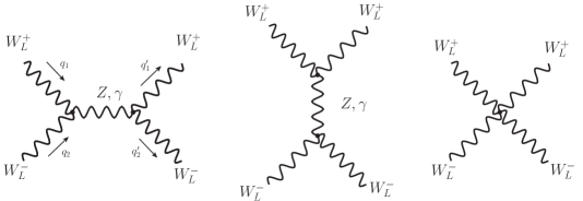
Figure 2: Feynman graphs from the gauge sector which contribute to tree-level W-boson scattering.

First, we consider the diagrams shown in Figure 2. Since the corresponding Feynman rules for the vertices are derived from the gauge sector, which is unchanged with respect to the SM, only the modified gauge-boson propagators (29) lead to a modification of the well-known SM result. Concerning the leading terms, growing with energy like $s^{2}$, the SM result is unchanged, i.e. these terms cancel in the sum of the three diagrams. As expected, the gauge-dependent pieces of the propagator do not contribute and the pure gauge-sector amplitude $\mathcal{M}_{\mathrm{GS}}$ is given by

$$\mathcal{M}_{\mathrm{GS}}=\frac{ig^{2}}{4m_{W}^{2}}\left[s\left(4-2\gamma(t)-\gamma(s)\right)+t\left(4-2\gamma(s)-\gamma(t)\right)\right]+\mathcal{O}(s^{0})\,,$$ (52)

where

$$\gamma(s)=\frac{\hat{m}_{W}^{2}}{m_{W}^{2}}\left(1+\frac{\Pi^{\mathrm{new}}_{Z}(s)}{\hat{m}_{Z}^{2}}\right)$$ (53)

and $\Pi^{\mathrm{new}}_{\mathrm{V}}(s)$ is the self-energy contribution defined in Eq.(32). For the Mandelstam prescription, the self-energy vanishes and the first factor reduces to unity, in which case Eq.(52) equals the SM result [2]. However, for the straight Wilson line, the SM result is modified as above.

In the SM longitudinal W-boson scattering is unitarized by Higgs-boson exchange. The corresponding Feynman graphs are shown in Figure 3. The relevant vertex function for the coupling of a single Higgs boson $\rho$ and two W bosons can be derived with the techniques described in Section 2 or from the general result in Appendix A, and reads

$$\Gamma_{W^{+}W^{-}\hat{\rho}}^{\mu\nu}(q_{1},q_{2})=\frac{g^{2}\tilde{v}}{4}\int_{0}^{1}ds_{1}\int_{0}^{s_{1}}ds_{2}\,\, \left\{\left[\frac{\partial}{\partial q_{\mu}}\frac{\partial}{\partial q_{\nu}}\tilde{F}\left(q^{2}\right)\right]_{q=p+q_{1}s_{1}+q_{2}s_{2}}\right.$$ (54)

$$\left.\!+\left[\frac{\partial}{\partial q_{\mu}}\frac{\partial}{\partial q_{\nu}}\tilde{F}\left(q^{2}\right)\right]_{q=q_{1}s_{1}+q_{2}s_{2}}\right\}\,,$$

where $q_{1}$ and $q_{2}$ are the W-boson momenta and $p=-q_{1}-q_{2}$ is the incoming momentum of the Higgs boson. This Feynman rule looks simple but the integrals cannot be generally performed without further knowledge on $\tilde{F}(p^{2})$. However, for a two-to-two scattering process the longitudinal polarization vectors of the gauge bosons can be expressed in a rather simple way in terms of the gauge-boson momenta. For example, one finds

$$\epsilon_{L}^{\mu}(q_{1})=\frac{1}{m_{W}\beta}\left(q_{1}^{\mu}-\frac{2m_{W}^{2}}{s}(q_{1}+q_{2})^{\mu}\right)=\frac{1}{m_{W}}\left(q_{1}^{\mu}-\frac{2m_{W}^{2}}{s}q_{2}^{\mu}\right)+\mathcal{O}\!\left(\frac{q_{1,2}^{\mu}}{m_{W}}\frac{m_{W}^{4}}{s^{2}}\right),$$ (55)

where $\beta=\sqrt{1-4m_{W}^{2}/s}$ and $\vec{q}_{1}=-\vec{q}_{2}$ has been used to establish the relation. Since in two-to-two scattering the three-momenta of the final-state particles satisfy $\vec{q}_{3}=-\vec{q}_{4}$, an equivalent relation is valid for all four polarization vectors. Hence, for the scattering of longitudinal gauge bosons, it is sufficient to compute $q_{i\mu}q_{j\nu}\Gamma_{W^{+}W^{-}\hat{\rho}}^{\mu\nu}$. Moreover, at high energies, the leading approximation to the polarizations vector is proportional to the momentum of the corresponding gauge boson, while the next-to-leading approximation involves the other initial- or final-state momentum.

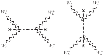
Figure 3: Feynman graphs for Higgs-boson exchange in analogy to the SM. The crosses indicate that a Higgs boson has been replaced by its vev.

Focusing on the leading approximation to the polarization vectors and the resulting leading terms in the amplitude, the vertex function contracted with the momenta of the gauge bosons can be expressed in terms of derivatives with respect to the integration variables, which parameterize the Wilson line,

$$q_{1\mu}q_{2\mu}\Gamma_{W^{+}W^{-}\hat{\rho}}^{\mu\nu}(q_{1},q_{2})=\frac{g^{2}\tilde{v}}{4}\int_{0}^{1}ds_{1}\int_{0}^{s_{1}}ds_{2}\,\,\frac{\partial}{\partial s_{1}}\frac{\partial}{\partial s_{2}} \left[\tilde{F}\left((q_{1}s_{1}+q_{2}s_{2})^{2}\right)\right.$$ (56)

$$+\left.\tilde{F}\left((q_{1}(s_{1}-1)+q_{2}(s_{2}-1))^{2}\right)\right]\,.$$

After combining the two terms by a straight-forward variable transformation, the integrals can be done and yield

$$q_{1\mu}q_{2\mu}\Gamma_{W^{+}W^{-}\hat{\rho}}^{\mu\nu}(q_{1},q_{2})= \frac{g^{2}\tilde{v}}{4}\left[\tilde{F}\left((q_{1}+q_{2})^{2}\right)+\tilde{F}(0)-2\tilde{F}(m_{W}^{2})\right]\,.$$ (57)

The corresponding leading piece of the amplitude reads

$$\mathcal{M}_{\mathrm{UH}}^{\mathrm{L,tot}}=\mathcal{M}_{\mathrm{UH}}^{\mathrm{L}}(s)+\mathcal{M}_{\mathrm{UH}}^{\mathrm{L}}(t)\,,$$ (58)

where

$$\mathcal{M}_{\mathrm{UH}}^{\mathrm{L}}(s)= -i\frac{g^{4}\tilde{v}^{2}}{16m_{W}^{4}}\frac{1}{\tilde{F}(s)-\tilde{F}(M_{H}^{2})}\left[\tilde{F}(s)-\tilde{F}(0)\right]^{2}\,$$ (59)

and we have used $\tilde{F}(m_{W}^{2})=\tilde{F}(0)$ since the difference is $\mathcal{O}(g^{2})$ in terms which do not grow with energy. We are interested in models in which $\tilde{F}(s)$ grows with energy but not faster than $s$, cf. Eq.(2). Hence, the potentially unitarity-violating terms from the diagrams in Figure 3 are given by

$$\mathcal{M}_{\mathrm{UH}}^{\mathrm{L,tot}}= -i\frac{g^{4}\tilde{v}^{2}}{16m_{W}^{4}}\left[\tilde{F}(s)+\tilde{F}(t)\right]+\mathcal{O}(s^{0})\,.$$ (60)

Only in the SM limit, in which  $\tilde{F}(s)+\tilde{F}(t)\to s+t+\mathcal{O}(s^{0})$, the terms rising with energy cancel those from the gauge sector.

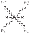
Figure 4: Four-gauge-boson two-Unhiggs vertex diagram. The crosses indicate that a Higgs boson has been replaced by its vev.

As has already been noted for the Mandelstam prescription [2], the diagram shown in Figure 4 contributes, which has no SM counterpart. Concentrating again on the leading terms of the polarization vectors, the corresponding vertex function contracted with momenta reads

$$q_{1\mu}q_{2\nu}q_{3\rho}q_{4\sigma}\Gamma_{4G}^{\mu\nu\rho\sigma}(q_{1},q_{2},q_{3},q_{4})=\,\, \frac{g^{4}\tilde{v}^{2}}{8}\int_{0}^{1}ds_{1}\int_{0}^{s_{1}}ds_{2}\int_{0}^{s_{2}}ds_{3}\int_{0}^{s_{3}}ds_{4}$$ (61)

$$\Bigg{[}\frac{\partial^{4}}{\partial s_{1}\partial s_{2}\partial s_{3}\partial s_{4}}\tilde{F}\left((q_{1}s_{1}+q_{2}s_{2}+q_{3}s_{3}+q_{4}s_{4})^{2}\right)+(q_{1}\leftrightarrow q_{3})+(q_{2}\leftrightarrow q_{4})+\left(\begin{array}[]{c}q_{1}\leftrightarrow q_{3}\\ q_{2}\leftrightarrow q_{4}\end{array}\right)\Bigg{]}\,.$$ (64)

Reordering integrations according to

$$\int_{0}^{1}ds_{1}\int_{0}^{s_{1}}ds_{2}\int_{0}^{s_{2}}ds_{3}\int_{0}^{s_{3}}ds_{4}=\int_{0}^{1}ds_{1}\int_{0}^{s_{1}}ds_{3}\int_{s_{3}}^{s_{1}}ds_{2}\int_{0}^{s_{3}}ds_{4}\,,$$ (65)

the last two integrals can be performed. In the remaining two-fold integral all terms in the integrand are either total derivatives with respect to one of the integrations or they depend only on a single integration variable after performing a suitable variable transformation. Hence, the result can be given in terms of one-dimensional integrals and the corresponding leading amplitude reads

$$\mathcal{M}_{\mathrm{4G}}^{\mathrm{L,tot}}=i\,\frac{q_{1\mu}}{m_{W}}\frac{q_{2\nu}}{m_{W}}\frac{q_{3\rho}}{m_{W}}\frac{q_{4\sigma}}{m_{W}}\,\Gamma_{4G}^{\mu\nu\rho\sigma}(q_{1},q_{2},q_{3},q_{4})=\mathcal{M}_{\mathrm{4G}}^{\mathrm{L}}(s,t)+\mathcal{M}_{\mathrm{4G}}^{\mathrm{L}}(t,s)\,,$$ (66)

where

$$\mathcal{M}_{\mathrm{4G}}^{\mathrm{L}}(s,t)=i\frac{g^{4}\tilde{v}^{2}}{8m_{W}^{4}} \Bigg{[}4s\,\frac{\tilde{F}(m_{W}^{2})-\tilde{F}(0)}{m_{W}^{2}}+\frac{1}{2}\left[\tilde{F}(s)-\tilde{F}(0)\right]$$ (67)

$$+\left(\frac{s}{2}+t\right)\left[\frac{\tilde{F}(s)-\tilde{F}(0)}{s}-2\int_{0}^{1}\!dx\,\tilde{F}^{(1)}(sx^{2})\right]-\left(t+2s\right)\int_{0}^{1}\!dx\,\tilde{F}^{(1)}\left(tx(x-1)\right)\Bigg{]}\,,$$

and we have neglected $m_{W}^{2}$ compared to $s$ or $t$ in factors multiplying $\tilde{F}(p^{2})$ as well as in its arguments. In contrast to the Mandelstam prescription, the contributions from this diagram do not cancel all the unitarity-violating terms rising with energy in the other diagrams. The last term even contains a new integrand which is not present in any of the previously calculated amplitudes.

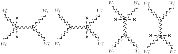
Figure 5: Additional graphs involving the two-Unhiggs triple gauge-boson vertex in combination with the SM triple gauge-boson vertex.

There is yet another class of diagrams, which can be shown not to contribute in the Mandelstam case, but turns out to be essential for the unitarity cancellation in the Wilson-line model. The relevant vertex results from the coupling of two Unhiggs fields with three gauge bosons when expanding the Wilson line to third order. The corresponding diagrams are shown in Figure 5. Since we are interested only in the terms which grow with energy, the masses in the propagators can be neglected such that we can calculate directly the exchange of the neutral SU(2) boson instead of a Z-boson and a photon.

The leading amplitude for the left diagram in Figure 5, again replacing the four polarization vectors by the corresponding momenta, is given by

$$\mathcal{M}^{\mathrm{L}}_{\mathrm{3G},1}= -i\frac{g^{4}\tilde{v}^{2}}{16m_{W}^{4}}\left(q_{3}-q_{4}\right)_{\rho}q_{1\mu}q_{2\nu}$$ (68)

$$\times\int_{0}^{1}ds_{1}\int_{0}^{s_{1}}ds_{2}\int_{0}^{s_{2}}ds_{3}\,\bigg{[}\tilde{F}^{\mu\nu\rho}(s_{1},s_{2},s_{3})-\tilde{F}^{\mu\nu\rho}(s_{1},s_{3},s_{2})+\tilde{F}^{\mu\nu\rho}(s_{2},s_{3},s_{1})\bigg{]}\,,$$

where

$$\tilde{F}^{\mu\nu\rho}(s_{1},s_{2},s_{3})= \left.\frac{\partial^{3}}{\partial q_{\mu}\partial q_{\nu}\partial q_{\rho}}\tilde{F}\left(q^{2}\right)\right|_{q=q_{1}s_{1}+q_{2}s_{2}+(q_{3}+q_{4})s_{3}}\,.$$ (69)

The denominator of the propagator has canceled against a term resulting from the algebra of the SM three-gauge-boson vertex and the gauge-dependent terms of the propagator do not contribute. The three terms in the Unhiggs vertex result from the path ordering of the fields and can be derived from the general result in Appendix A by setting the Higgs fields to their vev and making the SU(2) gauge fields explicit. Since $\tilde{F}^{\mu\nu\rho}(p^{2})$ is again contracted with momenta, we can rewrite all derivatives as derivatives with respect to the integration variables, e.g.

$$q_{1\mu}q_{2\nu}q_{3\rho}\tilde{F}^{\mu\nu\rho}(s_{1},s_{2},s_{3})=\frac{\partial}{\partial s_{1}}\frac{\partial}{\partial s_{2}}\left[\frac{\partial}{\partial s_{3}}\tilde{F}\left((q_{1}s_{1}+q_{2}s_{2}+q_{3}s_{3}+q_{4}s_{4})^{2}\right)\right]_{s_{4}=s_{3}}\,.$$ (70)

The six three-fold integrals for each of the four diagrams (most of them related by permutation of the momenta) can be again reduced to one-fold integrals and the combined result reads

$$\mathcal{M}^{\mathrm{L,tot}}_{\mathrm{3G}}=\mathcal{M}^{\mathrm{L}}_{\mathrm{3G}}(s,t)+\mathcal{M}^{\mathrm{L}}_{\mathrm{3G}}(t,s)\,,$$ (71)

where

$$\mathcal{M}^{\mathrm{L}}_{\mathrm{3G}}(s,t)=-i\frac{g^{4}\tilde{v}^{2}}{8m_{W}^{4}} \Bigg{\{}2\left(s+2t\right)\frac{\tilde{F}(m_{W}^{2})-\tilde{F}(0)}{m_{W}^{2}}$$ (72)

$$-\left(s+2t\right)\int_{0}^{1}dx\tilde{F}^{(1)}\left(s(x-1)x\right)+\left(s+2t\right)\Bigg{[}\frac{\tilde{F}\left(s\right)-\tilde{F}(0)}{s}-2\int_{0}^{1}dx\tilde{F}^{(1)}\!\left(sx^{2}\right)\Bigg{]}\Bigg{\}}\,.$$

As before, we neglected $m_{W}^{2}$ compared to terms of order $s$.

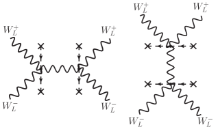
Figure 6: Additional graphs resulting from two two-Unhiggs triple gauge-boson vertices.

The last class of diagrams to consider is displayed in Figure 6. In order to show that these two diagrams do not contribute to the unitarization of W-boson scattering, we have to further investigate the vertices. Each vertex is connected to two external lines and the corresponding Lorentz indices are again contracted with the momenta of the external bosons in the leading approximation. With one open Lorentz index, we now have to evaluate

$$q_{1\mu}q_{2\nu}\Gamma_{3G}^{\mu\nu\rho} \propto \,q_{1\mu}q_{2\nu}\int_{0}^{1}ds_{1}\int_{0}^{s_{1}}ds_{2}\int_{0}^{s_{2}}ds_{3}\,$$ (73)

$$\bigg{[}\tilde{F}^{\mu\nu\rho}(s_{1},s_{2},s_{3})-\tilde{F}^{\mu\nu\rho}(s_{1},s_{3},s_{2})+\tilde{F}^{\mu\nu\rho}(s_{2},s_{3},s_{1})\bigg{]}\,.$$

The second term is easily calculated because the integrand is a total derivative with respect to both the $s_{1}$ and $s_{3}$ integrations. Hence, the integrand of the remaining $s_{2}$ integration is proportional to $\tilde{F}^{(1)}(p^{2})$ and a sum of uncontracted momentum vectors. Since we are only concerned with kernels for which $\tilde{F}^{(1)}(p^{2})$ goes to zero when $p^{2}$ becomes large, these terms rise with energy at most like a single momentum. For the first and the third term, the integrand is a total derivative with respect to the $s_{2}$ integration. For example, the first term results in

$$q_{1\mu}q_{2\nu}\int_{0}^{1}ds_{1}\int_{0}^{s_{1}}ds_{3} \int_{s_{3}}^{s_{1}}ds_{2}\,\tilde{F}^{\mu\nu\rho}(s_{1},s_{2},s_{3})=$$ (74)

$$q_{1\mu}\int_{0}^{1}ds_{1}\int_{0}^{s_{1}}ds_{3}\,\tilde{F}^{(2)}\left((s_{1}-s_{3})^{2}(q_{1}+q_{2})^{2}\right)4(s_{1}-s_{3})^{2}(q_{1}+q_{2})^{\mu}(q_{1}+q_{2})^{\rho}$$

$$-q_{1\mu}\int_{0}^{1}ds_{1}\!\!\int_{0}^{s_{1}}ds_{3}\,\tilde{F}^{(2)}\left((s_{1}-s_{3})^{2}q_{1}^{2}\right)4(s_{1}-s_{3})^{2}q_{1}^{\mu}q_{1}^{\rho}+\ldots\,,$$

where we have used momentum conservation in the vertex and omitted terms which only contain first derivatives of $\tilde{F}$ and are not dangerous at high energies. Changing integration variables to $(s_{1}-s_{3})$ and integrating by parts, we again derive a result which contains only first derivatives of $\tilde{F}$. The first term again rises with energy only like a single momentum, because partial integration yields a large suppression factor $(q_{1}+q_{2})^{2}\sim s$ in the denominator. The second term is potentially more dangerous at high energies because one finds a factor $q_{1}^{2}=m^{2}_{W}$ in the denominator and three momenta in the numerator. This behaviour follows from Eq.(74) since the argument of $\tilde{F}^{(2)}\left((s_{1}-s_{3})^{2}m_{W}^{2}\right)$ does not rise with energy and cannot suppress the integrand at large energies when the momenta in the numerator become large. However, as also seen from the equation, dotting $q_{1}$ into the vertex converts momentum factors into the small quantity $m_{W}^{2}$. It is a generic feature that the terms in the vertices which potentially rise fastest with energy are tamed by explicit factors of $m_{W}^{2}$ in the numerator. Hence, the vertex contracted with the external momenta only rises with energy like a single momentum. It follows that the diagrams in Figure 6, which are built by two of these contracted vertices and a propagator do not lead to unitarity-violating terms in the amplitude. The diagrams in Figure 5 do contribute because the SM vertex contracted with external momenta rises like the third power of the centre-of-mass energy.

Adding up all terms the complete leading amplitude from the SM and Unhiggs diagrams is given by

$$\mathcal{M}^{\mathrm{L,tot}}= \,\,\mathcal{M}_{\mathrm{GS}}+\mathcal{M}^{\mathrm{L,tot}}_{\mathrm{UH}}+\mathcal{M}^{\mathrm{L,tot}}_{\mathrm{4G}}+\mathcal{M}^{\mathrm{L,tot}}_{\mathrm{3G}}$$ (75)

$$= \,\,i\frac{g^{4}\tilde{v}^{2}}{8m_{W}^{4}}\left[4(s+t)\left(\int_{0}^{1}dx\tilde{F}^{(1)}(m_{W}^{2}x^{2})-\frac{\tilde{F}(m_{W}^{2})-\tilde{F}(0)}{m_{W}^{2}}\right)\right.$$

$$+\tilde{F}(0)-\tilde{F}(M_{H}^{2})\left.-\frac{1}{2}\left(\frac{(\tilde{F}(0)-\tilde{F}(M_{H}^{2}))^{2}}{\tilde{F}(s)-\tilde{F}(M_{H}^{2})}+\frac{(\tilde{F}(0)-\tilde{F}(M_{H}^{2}))^{2}}{\tilde{F}(t)-\tilde{F}(M_{H}^{2})}\right)\right]+\mathcal{O}\!\left(g^{2}\right)\,,$$

where we have kept all terms which rise with energy or do not go to zero in the limit of vanishing gauge couplings. Most of the potentially unitarity-violating terms in the different diagrams have indeed canceled. However, the terms in the first line still violate unitarity at high energies.

As we show in the following, the unitarity restoration occurs in the present non-local Higgs theory only when sub-leading terms in the longitudinal polarization vectors Eq.(55) are included. The critical diagrams are those from Figures 4 and 5 from the triple and quartic gauge-boson vertex in the Unhiggs sector. Substituting the sub-leading term from Eq.(55) in one of the four polarization vectors in the quartic gauge-boson vertex diagram and summing over the four possibilities, the next-to-leading amplitude is given by

$$\mathcal{M}_{\mathrm{4G}}^{\mathrm{NL,tot}}=\frac{-2i}{sm_{W}^{2}}\left[\left(q_{1\mu}q_{1\nu}+q_{2\mu}q_{2\nu}\right)q_{3\rho}q_{4\sigma}+q_{1\mu}q_{2\nu}\left(q_{3\rho}q_{3\sigma}+q_{4\rho}q_{4\sigma}\right)\right]\Gamma_{4G}^{\mu\nu\rho\sigma}(q_{1},q_{2},q_{3},q_{4})\,.$$ (76)

As for the leading amplitude two integrations inside the vertex can always be trivially performed. The discussion after Eq.(74) shows that only terms including $\tilde{F}^{(2)}((s_{i}-s_{j})m_{W}^{2})$ can contribute because of the extra factor $1/s$ in the next-to-leading amplitude. All these terms can be further integrated and yield

$$\mathcal{M}_{\mathrm{4G}}^{\mathrm{NL,tot}}= \,\,i\frac{g^{4}\tilde{v}^{2}}{m_{W}^{4}}(s+t)\left(\int_{0}^{1}dx\,\tilde{F}^{(1)}(m_{W}^{2}x^{2})-\frac{\tilde{F}(m_{W}^{2})-\tilde{F}(0)}{m_{W}^{2}}\right)\,.$$ (77)

The equivalent analysis of the next-to-leading terms for the diagrams in Figure 5 results in

$$\mathcal{M}_{\mathrm{3G}}^{\mathrm{NL,tot}}=\mathcal{M}_{\mathrm{3G}}^{\mathrm{NL}}(s,t)+\mathcal{M}_{\mathrm{3G}}^{\mathrm{NL}}(t,s)\,$$ (78)

where

$$\mathcal{M}_{\mathrm{3G}}^{\mathrm{NL}}(s,t)=-i\frac{g^{4}\tilde{v}^{2}}{2m_{W}^{4}}(s+2t)\left(\int_{0}^{1}dx\,\tilde{F}^{(1)}(m_{W}^{2}x^{2})-\frac{\tilde{F}(m_{W}^{2})-\tilde{F}(0)}{m_{W}^{2}}\right)\,.$$ (79)

The diagrams in Figure 6 once again do not contribute to the terms rising with energy. There are a few terms appearing in the evaluation of $\mathcal{M}_{\mathrm{4G}}^{\mathrm{NL,tot}}$ and $\mathcal{M}_{\mathrm{3G}}^{\mathrm{NL,tot}}$ which cannot be rewritten in terms of one-fold integrals. Hence, it is not obvious for a general kernel that these terms do not contribute. However, when adding these terms from the different sets of diagrams we find that they cancel exactly.

Finally, adding up all the leading and next-to-leading terms, all unitarity-violating terms cancel. That is, quite remarkably, the left-over terms in the second line of Eq.(75) are indeed canceled by those from the next-to-leading terms in the polarization vectors. Since next-to-next-to-leading terms in the expansion of the longitudinal polarization vectors are suppressed by another factor of $m_{W}^{2}/s$ and cannot contribute to potentially unitarity-violating terms, this completes the explicit demonstration that high-energy unitarity is not spoiled by the non-local Higgs sector. We further note that non-leading pieces in all the diagrams related to the Unhiggs sector do not contribute at $\mathcal{O}(g^{0})$, in contrast to non-leading pieces in the SM like diagrams which are already included. Hence, the final result for the amplitude reads

$$\mathcal{M}\!= \frac{-i}{\tilde{F}^{(1)}(0)^{2}}\!\left[\,2V^{(2)}(\tilde{v}^{2}/2)+\tilde{v}^{2}\,(V^{(2)}(\tilde{v}^{2}/2))^{2}\!\left(\frac{1}{\tilde{F}(s)-\tilde{F}(M_{H}^{2})}+\frac{1}{\tilde{F}(t)-\tilde{F}(M_{H}^{2})}\right)\,\right]\!\!+\mathcal{O}(g^{2})\,,$$ (80)

where we have used Eq.(15) and the relations between the different mass parameters $\tilde{m}^{2}_{W}=g^{2}\tilde{v}^{2}/4=\hat{m}^{2}_{W}/\tilde{F}^{(1)}(0)=m_{W}^{2}/\tilde{F}^{(1)}(0)\times[1+\mathcal{O}(g^{2})]$.

5.2 Comparison to minimal coupling

As we have shown in the previous section, unitarization of longitudinal W-boson scattering does not only take place for a minimally coupled action but also for an action based on the straight Wilson line. While the cancellation of potentially unitarity violating terms is based in both cases on the non-trivial interplay of different diagrams, the cancellation for the straight Wilson line is more involved, and additionally involves the graphs in Figure 5.

The terms (80) remaining in the limit of vanishing gauge couplings are identical for the minimally coupled and Wilson-line actions. Using the non-local kernel (2) and the Higgs potential (16), our result Eq.(80) matches the result in Eq. (3.29) of Ref. [2]. This coincidence of results is certainly not accidental and suggests that the Goldstone-boson equivalence theorem applies to non-local Higgs actions as we verify below. The left-over terms in Eq.(80) imply as usual constraints on the Higgs potential, since the energy-independent terms must not be too large to satisfy unitarity. However, since there is no difference to the minimal-coupling result discussed in Ref. [2], we do not repeat the corresponding analysis of constraints on $d$ and $\mu$ here.

5.3 Goldstone-boson equivalence theorem

In the SM the Goldstone-boson equivalence theorem [15, 16, 17] for longitudinal W-boson scattering reads

$$\mathcal{M}\left[W^{+,L}(p_{1})+W^{-,L}(p_{2})\to W^{+,L}(p^{\prime}_{1})+W^{-,L}(p^{\prime}_{2})\right]$$ (81)

$$\quad=\,\mathcal{M}\left[\pi^{+}(p_{1})+\pi^{-}(p_{2})\to\pi^{+}(p^{\prime}_{1})+\pi^{-}(p^{\prime}_{2})\right]+\mathcal{O}\left(\frac{m_{W}}{E}\right)\,,$$

i.e. at high energies the longitudinal W boson scattering amplitude equals the scattering amplitude of the corresponding Goldstone bosons up to terms that vanish in the high-energy limit. In the following, we again consider the limit of vanishing gauge couplings, in which the terms of order $m_{W}/E$ vanish and the two amplitudes are predicted to agree precisely.

In this work, we do not attempt a formal proof of the Goldstone-boson equivalence theorem for non-local Higgs-gauge theories but verify it by a tree-level calculation of the Goldstone scattering amplitude on the right hand side of Eq.(81). That the theorem is likely to be valid in the present class of non-local theories can be understood by the following considerations: Since we are not considering corrections due to the gauge couplings, we can set $m_{\mathrm{V}}=\hat{m}_{\mathrm{V}}$. The gauge-fixing condition (25) is then identical to SM $R_{\xi}$-gauge. Hence, the resulting Ward identity, which is the cornerstone of formal proofs [17, 18] of the equivalence theorem, can be expected to hold unmodified for the non-local Higgs model. Moreover, as shown above the propagators for the longitudinal gauge bosons and the Goldstone bosons only differ by a factor of $\xi$ (as in the SM), so the Ward identity for connected Green functions can be translated into an identity for matrix elements, which yields the desired result.

The calculation of the amplitude for charged Goldstone-boson scattering $\pi^{+}\pi^{-}\to\pi^{+}\pi^{-}$ in the limit of vanishing gauge couplings depends only on the Higgs potential (9). By expanding the Higgs potential to second order around the vev, the interaction terms relevant to charged Goldstone scattering at tree-level are given by

$$S\supset-\int d^{4}x\,\frac{1}{2}\,\frac{V^{(2)}(\tilde{v}^{2}/2)}{\tilde{F}^{(1)}(0)^{2}}\left(2v\,\rho\,\pi^{+}\pi^{-}+(\pi^{+}\pi^{-})^{2}\right)\,.$$ (82)

The Feynman rules for the triple and quartic scalar interaction vertices can be deduced from this expression. The calculation of the tree-level Goldstone scattering amplitude is straight-forward resulting in

$$\mathcal{M}= -i\left[\,2\,\frac{V^{(2)}(\tilde{v}^{2}/2)}{\tilde{F}^{(1)}(0)^{2}}+v^{2}\left(\frac{V^{(2)}(\tilde{v}^{2}/2)}{\tilde{F}^{(1)}(0)^{2}}\right)^{\!2}\left(\frac{\tilde{F}^{(1)}(0)}{\tilde{F}(s)-\tilde{F}(M_{H}^{2})}+\frac{\tilde{F}^{(1)}(0)}{\tilde{F}(t)-\tilde{F}(M_{H}^{2})}\right)\right]\,.$$ (83)

The first term is due to the vertex with four charged Goldstone bosons. The remaining two stem from the $s$- and $t$-channel exchange of the physical Higgs boson, respectively. Using $v^{2}=\tilde{v}^{2}\tilde{F}^{(1)}(0)$, the longitudinal WW scattering amplitude (80) and Eq.(83) indeed agree as they should, if the Goldstone-boson equivalence theorem holds.

6 Summary

The present work has been motivated by the observation made in Ref. [2] that the standard mechanism of electroweak symmetry breaking by the Higgs field can be made to work when the Higgs action is non-local. While the specific form of the action (1), and the assumption that only the Higgs sector is non-local may be hard to justify from the viewpoint of model-building, the fact that a radical modification from the standard set-up such as relinquishing locality appears to be consistently unitarizing the theory at energies above the symmetry-breaking scale is certainly interesting.

In previous work a minimal-coupling prescription has been employed to render the theory gauge-invariant, but this is far from unique when the action is non-local and cannot be expanded into a series of local operators of increasing dimension. Here we considered non-local theories with general kernels and gauge invariance maintained by a straight Wilson line extended between the positions of the Higgs fields. One of our main findings is that longitudinal WW scattering unitarizes, but as a consequence of diagrammatic cancellations that are remarkably non-trivial compared to the SM and even to the minimally-coupled non-local Higgs model. We verified that the Goldstone-boson equivalence theorem is fulfilled and suggest that its formal proof should be extensible to the non-local case.

For particle physics model building the model does not look promising, however. Contrary to Ref. [2], we find that the quantum corrections to the Higgs mass are not reduced (unless the dimension of the Higgs field is very close to the pathological limit $d=2$), when expressed in terms of known low-energy parameters, and hence the model does not reduce the (little) hierarchy problem in the sense of allowing a larger cut-off than the SM for the same amount of cancellations in the Higgs self-energy. Furthermore, unlike the minimally-coupled theory, in general there exist tree-level corrections to the transverse gauge-boson propagators, leading to unacceptably large values of the $S$-parameter and the W-mass shift, unless the scale $\mu$ of non-locality is significantly larger than the electroweak scale, or $d$ is close to the SM limit $d=1$. But sufficiently below the scale $\mu$ the non-local Higgs sector is indistinguishable from the standard local implementation.

Acknowledgement

We thank M. Luty, J. Rohrwild and J. Terning for useful discussions. MB thanks the Kavli Institute for Theoretical Physics at UC Santa Barbara for hospitality, while part of this work was done. This work is supported in part by the Gottfried Wilhelm Leibniz programme of the Deutsche Forschungsgemeinschaft (DFG) and by the National Science Foundation under Grant No. NSF PHY05-51164.

Appendix A Generic interactions

In this appendix the interaction terms for the straight Wilson-line coupling of the non-local Higgs sector to the gauge fields are derived. Expanding the path-ordered exponential, the action (3) is given by

$$S\supset \int d^{4}x\int d^{4}y\,F(x-y)$$ (84)

$$\times\sum_{n=1}^{\infty}\,(-ig)^{n}\int_{y}^{x}dz_{1,\nu_{1}}\int_{y}^{z_{1}}dz_{2,\nu_{2}}\cdots\int_{y}^{z_{n-1}}dz_{n,\nu_{n}}\,\phi^{\dagger}(x)\,A^{\nu_{1}}(z_{1})\cdots A^{\nu_{n}}(z_{n})\,\phi(y)\,,$$

where $A^{\nu_{n}}(z_{n})=\tau^{a_{n}}A^{\nu_{n}}_{a_{n}}(z_{n})$ is the matrix-valued gauge field of the gauge group under consideration. Note that the definition of the path-ordered exponential does not include factors of $1/n!$. For the straight Wilson line, the path is parameterized by $z^{\nu}_{n}=(x-y)^{\nu}s_{n}+y^{\nu}$ yielding

$$S\supset \int d^{4}x\int d^{4}y\,F(x-y)\,\sum_{n=1}^{\infty}\,(-ig)^{n}\int_{0}^{1}ds_{1}\,(x-y)_{\nu_{1}}$$ (85)

$$\times\int_{0}^{s_{1}}ds_{2}\,(x-y)_{\nu_{2}}\cdots\int_{0}^{s_{n-1}}ds_{n}\,(x-y)_{\nu_{n}}\,\phi^{\dagger}(x)\,A^{\nu_{1}}(s_{1})\cdots A^{\nu_{n}}(s_{n})\,\phi(y)\,.$$

In momentum space the action is then given by

$$S\supset \sum_{n=1}^{\infty}\,(-ig)^{n}\int\frac{d^{4}q}{(2\pi)^{4}}\frac{d^{4}p_{1}}{(2\pi)^{4}}\frac{d^{4}p_{2}}{(2\pi)^{4}}\frac{d^{4}q_{1}}{(2\pi)^{4}}\cdots\frac{d^{4}q_{n}}{(2\pi)^{4}}\,\tilde{F}(q^{2})\,\phi^{\dagger}(p_{1})A^{\nu_{1}}(q_{1})\cdots A^{\nu_{n}}(q_{n})\,\phi(p_{2})$$

$$\times\frac{i\partial}{\partial q^{\nu_{1}}}\cdots\frac{i\partial}{\partial q^{\nu_{n}}}\int\!d^{4}x\!\int\!d^{4}y\!\int_{0}^{1}\!\!\!ds_{1}\cdots\!\int_{0}^{s_{n-1}}\!\!\!\!\!ds_{n}\,e^{-ix(q-p_{1}+\sum_{k=1}^{n}s_{k}q_{k})}e^{+iy(q-p_{2}+\sum_{k=1}^{n}(s_{k}-1)q_{k})}\,.$$ (86)

Performing the integrations over the variables $x$ and $y$, using partial integration and finally performing the $q$-integration, we find

$$S\supset \sum_{n=1}^{\infty}\,g^{n}\int\frac{d^{4}p_{1}}{(2\pi)^{4}}\frac{d^{4}p_{2}}{(2\pi)^{4}}\frac{d^{4}q_{1}}{(2\pi)^{4}}\cdots\frac{d^{4}q_{n}}{(2\pi)^{4}}\,\phi^{\dagger}(-p_{1})A^{\nu_{1}}(q_{1})\cdots A^{\nu_{n}}(q_{n})\,\phi(p_{2})$$ (87)

$$\times(2\pi)^{4}\delta^{(4)}\left(p_{1}+p_{2}+\sum_{k=1}^{n}q_{k}\right)\int_{0}^{1}ds_{1}\,\cdots\int_{0}^{s_{n-1}}ds_{n}\,\,\left.\frac{\partial}{\partial q^{\nu_{1}}}\cdots\frac{\partial}{\partial q^{\nu_{n}}}\tilde{F}(q^{2})\right|_{q=p_{1}+\sum_{k=1}^{n}s_{k}q_{k}}\,.$$

This expression allows us to read off the Feynman rule for a vertex with two Higgs and any number of gauge fields. For the specific case of the electroweak gauge group, where one is interested in the interactions of the physical Higgs field and the Goldstone modes with photons, W- and Z-bosons, one can easily make the group factors, hidden in the matrix notation for the gauge fields and the Higgs doublets, explicit. Feynman rules involving the Higgs vacuum expectation value are obtained by setting the momentum of the corresponding Higgs field to zero.

References

• [1] H. Georgi, Phys. Rev. Lett.  98 (2007) 221601, hep-ph/0703260.
• [2] D. Stancato, J. Terning, JHEP 0911 (2009) 101, arXiv:0807.3961 [hep-ph].
• [3] A. Falkowski, M. Perez-Victoria, Phys. Rev.  D79 (2009) 035005, arXiv:0810.4940 [hep-ph].
• [4] G. Cacciapaglia, G. Marandella, J. Terning, JHEP 0902 (2009) 049, arXiv:0804.0424 [hep-ph].
• [5] A. Falkowski, M. Perez-Victoria, JHEP 0812 (2008) 107, arXiv:0806.1737 [hep-ph].
• [6] L. Randall, R. Sundrum, Phys. Rev. Lett.  83 (1999) 3370-3373, hep-ph/9905221.
• [7] S. Mandelstam, Annals Phys.  19 (1962) 1-24.
• [8] J. Galloway, D. Martin, D. Stancato, arXiv:0802.0313 [hep-th].
• [9] A. Ilderton, Phys. Rev.  D79 (2009) 025014, arXiv:0810.3916 [hep-th].
• [10] A. L. Licht, arXiv:0802.4310 [hep-th].
• [11] A. L. Licht, arXiv:0806.3596 [hep-th].
• [12] A. L. Licht, arXiv:0805.3849 [hep-th].
• [13] M. E. Peskin, T. Takeuchi, Phys. Rev.  D46 (1992) 381-409.
• [14] K. Nakamura et al. [ Particle Data Group Collaboration ], J. Phys. G G37 (2010) 075021.
• [15] J. M. Cornwall, D. N. Levin, G. Tiktopoulos, Phys. Rev.  D10 (1974) 1145.
• [16] B. W. Lee, C. Quigg, H. B. Thacker, Phys. Rev.  D16 (1977) 1519.
• [17] M. S. Chanowitz, M. K. Gaillard, Nucl. Phys.  B261 (1985) 379.
• [18] G. J. Gounaris, R. Kögerler, H. Neufeld, Phys. Rev.  D34 (1986) 3257.