Turbo Lattices: Construction and Error Decoding Performance

Abstract

In this paper a new class of lattices called turbo lattices is introduced and established. We use the lattice Construction D to produce turbo lattices. This method needs a set of nested linear codes as its underlying structure. We benefit from turbo codes as our basis codes. Therefore, a set of nested turbo codes based on nested interleavers (block interleavers) and nested convolutional codes is built. To this end, we employ both tail-biting and zero-tail convolutional codes. Using these codes, along with construction D, turbo lattices are created. Several properties of Construction D lattices and fundamental characteristics of turbo lattices including the minimum distance, coding gain and kissing number are investigated. Furthermore, a multi-stage turbo lattice decoding algorithm based on iterative turbo decoding algorithm is given. We show, by simulation, that turbo lattices attain good error performance within $\sim 1.25~{}\mbox{dB}$ from capacity at block length of $n=1035$. Also an excellent performance of only $\sim.5~{}\mbox{dB}$ away from capacity at SER of $10^{-5}$ is achieved for size $n=10131$.

I Introduction

Turbo codes were first introduced by Berrou et al. [5] in 1993 and have been largely treated since then. It has been shown [19] that these codes with an iterative turbo decoding algorithm can achieve a very good error performance close to Shannon capacity. Also, there has been interest in constructing lattices with high coding gain, low kissing number and low decoding complexity [1, 21, 28]. The lattice version of the channel coding is to find an $n$-dimensional lattice $\Lambda$ which attains good error performance for a given value of volume-to-noise ratio (VNR) [10, 12, 31]. Poltyrev [20] suggests employing coding without restriction for lattices on the AWGN channel. This means communicating with no power constraints. The existence of ensembles of lattices which can achieve generalized capacity on the AWGN channel without restriction is also proved in [20]. Forney et al. [12] restate the above concepts by using coset codes and multilevel coset codes. At the receiver of communication without restriction for lattices, the main problem is to find the closest vector of $\Lambda$ to a given point ${\bf r}\in\mathbb{R}^{n}$. This is called lattice decoding of $\Lambda$. Some efficient well-known lattice decoders are known for low dimensions [14, 32].

There are a wide range of applicable lattices in communications including the well-known root lattices [10], the recently introduced low-density parity-check lattices [21] (LDPC lattices) and the low-density lattice codes [28] (LDLC lattices). The former lattices have been extensively treated in the 1980’s and 1990’s [10]. After the year 2000, two classes of lattices based on the primary idea of LDPC codes have been established. These type of lattices have attracted a lot of attention in recent years [1, 9, 22, 16]. Hence, constructing lattices based on turbo codes can be a promising research topic.

In the present work, we borrow the idea of turbo codes and construct a new class of lattices that we called turbo lattices. In fact, the results by Forney et al. in [12] motivate us to apply Construction D lattices to design turbo lattices. They proved the existence of sphere-bound-achieving lattices by means of Construction D lattices. This leads one to use Construction D method along with well-known turbo codes to produce turbo lattices. This is the first usage of turbo codes in constructing lattices. We benefit from structural properties of lattices and turbo codes to investigate and evaluate the basic parameters of turbo lattices such as minimum distance, volume, coding gain and kissing number.

Various types of turbo codes have been constructed in terms of properties of their underlying constituent encoders and interleavers [19]. For example, encoders can be either block or convolutional codes and interleavers can be deterministic, pseudo-random or random [33]. Since Construction D deals with block codes, we treat turbo codes as block codes. Therefore, it seems more reasonable to use terminated convolutional codes. Since we use recursive and non-recursive convolutional codes, different types of termination methods can be applied to these component convolutional codes. Hence, we are interested in terminating trellises for both feed-back [27, 34] and feed-forward [19] convolutional codes. To stay away from rate loss, we employ tail-biting convolutional codes for short length turbo lattices. Also zero-tail convolutional codes [27, 34] are building blocks of turbo codes to use in construction of lattices with larger sizes.

There are algorithms such as generalized min-sum algorithm [21], iterative decoding algorithms [9] and the algorithm in [28] for decoding newly introduced lattices. The basic idea behind these algorithms is to implement min-sum and sum-product algorithms and their generalizations. Since we used turbo codes to construct turbo lattices, it is more reasonable to benefit from the underlying turbo structure of these lattices. In this case, we have to somehow relate the decoding of turbo lattices to the iterative turbo decoders [5] for turbo codes. This results in a multi-stage decoding algorithm based on iterative turbo decoders similar to the one given in [12].

We summarize our contributions as follows.

• We generalize the minimum distance formula for every Construction D lattice by removing a restricting condition on the minimum distance of its underlying codes. An upper bound for the kissing number of these lattices is also derived.

• We construct nested turbo codes and establish the concept of turbo lattices. Various crucial parameters of these lattices such as minimum distance, coding gain and kissing number are investigated.

• A multi-stage turbo lattice decoder is introduced. The error performance of turbo lattices is given and compared with other well-known LDPC lattices and LDLC lattices.

The present work is organized as follow. Two methods of constructing lattices, Construction A and D, are reviewed in Section II. The crucial parameters of lattices which can be used to measure the efficiency of lattices are explained in this section. In Section III we introduce nested interleavers in a manner that can be used to build nested turbo codes. Section IV is devoted to the construction of nested turbo codes and consequently the construction of turbo lattices. Section V is dedicated to the evaluation of the critical parameters of turbo lattices based on the properties of their underlying turbo codes. In Section VI a multi-stage turbo lattice decoding algorithm is explained. In Section VII we carry simulation results. We conclude with final remarks on turbo lattices and further research topics in Section VIII.

II Backgrounds on Lattices

In order to make this work self-contained, a background on lattices is essential. The general required information about critical parameters of Construction A and Construction D as well as parameters for measuring the efficiency of lattices are provided below.

II-A General Notations for Lattices

A discrete additive subgroup $\Lambda$ of $\mathbb{R}^{n}$ is called lattice. Since $\Lambda$ is discrete, it can be generated by $m\leq n$ linearly independent vectors ${\bf b}_{1},\ldots,{\bf b}_{m}$ in $\mathbb{R}^{n}$. The set $\{{\bf b}_{1},\ldots,{\bf b}_{m}\}$ is called a basis for $\Lambda$. In the rest of this paper, we assume that $\Lambda$ is an $n$-dimensional full rank ($m=n$) lattice over $\mathbb{R}^{n}$. By using the Euclidean norm, $\|.\|$, we can define a metric on $\Lambda$; that is, for every ${\bf x},{\bf y}\in\Lambda$ we have $d({\bf x},{\bf y})=\|{\bf x}-{\bf y}\|^{2}$. The minimum distance of $\Lambda$, $d_{\min}(\Lambda)$, is

$$d_{\min}(\Lambda)=\min_{{\bf x}\neq{\bf y}}\{d({\bf x},{\bf y})|{\bf x},{\bf y}\in\Lambda\}.$$

Let us put $\{{\bf b}_{1},\ldots,{\bf b}_{n}\}$ as the rows of a matrix ${\bf B}$, then we have $\Lambda=\{{\bf x}\colon{\bf x}={\bf z}{\bf B},~{}{\bf z}\in\mathbb{Z}^{n}\}$. The matrix ${\bf B}$ is called a generator matrix for the lattice $\Lambda$. The volume of a lattice $\Lambda$ can be defined by $\det\left({\bf B}{\bf B}^{T}\right)$ where ${\bf B}^{T}$ is the transpose of ${\bf B}$. The volume of $\Lambda$ is denoted by $\det(\Lambda)$. The coding gain of a lattice $\Lambda$ is defined by

$$~{}\gamma(\Lambda)=\frac{d_{\min}^{2}(\Lambda)}{\det(\Lambda)^{2/n}},$$ (1)

where $\det(\Lambda)^{2/n}$ is itself called the normalized volume of $\Lambda$. This volume may be regarded as the volume of $\Lambda$ per two dimensions. The coding gain can be used as a crude measure of the performance of a lattice. For any $n$, $\gamma\left(\mathbb{Z}^{n}\right)=1$. An uncoded system may be regarded as the one that uses a constellation based on $\mathbb{Z}^{n}$. Thus the coding gain of an arbitrary lattice $\Lambda$ may be considered as the gain using a constellation based on $\Lambda$ over an uncoded system using a constellation based on $\mathbb{Z}^{n}$ [12]. Therefore, coding gain is the saving in average of energy due to using $\Lambda$ for the transmission instead of using the lattice $\mathbb{Z}^{n}$ [13]. Geometrically, coding gain measures the increase in density of $\Lambda$ over integer lattice $\mathbb{Z}^{n}$ [10].

If one put an $n$-dimensional sphere of radius $d_{\min}(\Lambda)/2$ centered at every lattice point of $\Lambda$, then the kissing number of $\Lambda$ is the maximum number of spheres that touch a fixed sphere. Hereafter we denote the kissing number of the lattice $\Lambda$ by $\tau(\Lambda)$. The normalized kissing number of an $n$-dimensional lattice $\Lambda$ is defined as

$$\tau^{\ast}(\Lambda)=\frac{\tau(\Lambda)}{n}.$$ (2)

Sending points of a specific lattice in the absence of power constraints has been studied. This is called coding without restriction [20]. Suppose that the points of an $n$-dimensional lattice $\Lambda$ are sent over an AWGN channel with noise variance $\sigma^{2}$. The volume-to-noise ratio (VNR) of an $n$-dimensional lattice $\Lambda$ is defined as

$$~{}{\alpha^{2}}=\frac{\det(\Lambda)^{\frac{2}{n}}}{2\pi e\sigma^{2}}.$$ (3)

For large $n$, the VNR is the ratio of the normalized volume of $\Lambda$ to the normalized volume of a noise sphere of squared radius $n\sigma^{2}$ which is defined as SNR in [21] and $\alpha^{2}$ in [12].

Since lattices have a uniform structure, we can assume ${\bf 0}$ is transmitted and r is the received vector. Then r is a vector whose components are distributed based on a Gaussian distribution with zero mean and variance $\sigma^{2}$. Hence construction of lattices with higher coding gain and lower normalized kissing number is of interest.

II-B Lattice Constructions

There exist many ways to construct a lattice [10]. In the following we give two algebraic constructions of lattices based on linear block codes [10]. The first one is Construction A which translates a block code to a lattice. Then a review of Construction D is given. These two constructions are the main building blocks of this work.

Let $\mathcal{C}$ be a group code over $G=\mathbb{Z}_{2}\times\cdots\times\mathbb{Z}_{2}$ , i.e. $\mathcal{C}\subseteq G$, with minimum distance $d_{\min}$. Define $\Lambda$ as a Construction A lattice [10] derived from $\mathcal{C}$ by:

$$\Lambda=\{(2z_{1}+c_{1},\ldots,2z_{n}+c_{n}):z_{i}\in\mathbb{Z},{\bf c}=(c_{1},\ldots,c_{n})\in\mathcal{C}\}.$$ (4)

Let $\Lambda$ be a lattice constructed using Construction A. The minimum distance of $\Lambda$ is

$$~{}d_{\min}(\Lambda)=\min\left\{2,\sqrt{d_{min}}\right\}.$$ (5)

Its coding gain is

$$~{}\gamma(\Lambda)=\left\{\begin{array}[]{ll}4^{\frac{k}{n}}&d_{\min}\geq 4,\\ \frac{d_{\min}^{2}(\Lambda)}{2}4^{\frac{k}{n}}&d_{\min}<4,\end{array}\right.$$ (6)

and its kissing number is

$$~{}\tau(\Lambda)=\left\{\begin{array}[]{ll}2^{d_{\min}}A_{d_{\min}}&d_{\min}<4,\\ 2n+16A_{4}&d_{\min}=4,\\ 2n&d_{\min}>4,\end{array}\right.$$ (7)

where $A_{d_{\min}}$ denotes the number of codewords in $\mathcal{C}$ with minimum weight $d_{\min}$. These definition and theorem can be generalized to a more practical and nice lattice construction. We use a set of nested linear block codes to give a more general lattice structure named Construction D. This construction plays a key role in this work.

Let $\mathcal{C}_{0}\supseteq\mathcal{C}_{1}\supseteq\cdots\supseteq\mathcal{C}_{a}$ be a family of $a+1$ linear codes where $\mathcal{C}_{\ell}[n,k_{\ell},d_{\min}^{(\ell)}]$ for $1\leq{\ell}\leq a$ and $\mathcal{C}_{0}$ is the $[n,n,1]$ trivial code $\mathbb{F}_{2}^{n}$ such that

$$\mathcal{C}_{\ell}=<{\bf c}_{1},\ldots,{\bf c}_{k_{\ell}}>$$

where $<X>$ denotes the subgroup generated by $X$. For any element ${\bf x}=(x_{1},\ldots,x_{n})\in\mathbb{F}^{n}_{2}$ and for $1\leq{\ell}\leq a$ consider the vector in $\mathbb{R}^{n}$ of the form:

$$\frac{1}{2^{{\ell}-1}}{\bf x}=\left(\frac{x_{1}}{2^{{\ell}-1}},\ldots,\frac{x_{n}}{2^{{\ell}-1}}\right).$$

Define $\Lambda\subseteq\mathbb{R}^{n}$ as all vectors of the form

$$~{}{\bf z}+\sum_{{\ell}=1}^{a}\sum_{j=1}^{k_{\ell}}\beta_{j}^{({\ell})}\frac{1}{2^{{\ell}-1}}{\bf c}_{j}$$ (8)

where ${\bf z}\in 2(\mathbb{Z})^{n}$ and $\beta_{j}^{({\ell})}=0$ or $1$. An integral basis for $\Lambda$ is given by the vectors

$$~{}\frac{1}{2^{{\ell}-1}}{\bf c}_{j}$$ (9)

for $1\leq{\ell}\leq a$ and $k_{{\ell}+1}+1\leq j\leq k_{\ell}$ plus $n-k_{1}$ vectors of the form $(0,\ldots,0,2,0,\ldots,0)$. Let us consider vectors ${\bf c}_{j}$ as integral in $\mathbb{R}^{n}$, with components $0$ or $1$. To be specific, this lattice $\Lambda$ can be represented by the following code formula

$$~{}\Lambda=\mathcal{C}_{1}+\frac{1}{2}\mathcal{C}_{2}+\cdots+\frac{1}{2^{a-1}}\mathcal{C}_{a}+2(\mathbb{Z})^{n}.$$ (10)

It is useful to bound the coding gain of $\Lambda$. The next theorem is cited form [4].

Theorem 1.

Let $\Lambda$ be a lattice constructed using Construction D, then the volume of $\Lambda$ is $\det(\Lambda)=2^{n-\sum_{{\ell}=1}^{a}k_{\ell}}$. Furthermore, if $d_{\min}^{(\ell)}\geq\frac{4^{\ell}}{\beta}$, for $1\leq{\ell}\leq a$ and $\beta=1$ or $2$, then the squared minimum distance of $\Lambda$ is at least $4/\beta$, and its coding gain satisfies

$$\gamma(\Lambda)\geq\beta^{-1}4^{\sum_{{\ell}=1}^{a}\frac{k_{\ell}}{n}}.$$

In the above theorem, an exact formula for the determinant of every lattice constructed using Construction D is given. Also, proper bounds for the other important parameters of these lattices including minimum distance and coding gain have been found with an extra condition on the minimum distance of the underlying nested codes [10].

We omit this restricting condition on the minimum distance of the underlying nested block codes and then generalize those bounds to a more useful form. The resulting expressions for minimum distance and coding gain are related to the underlying codes as we will see soon. In addition, an upper bound for the kissing number of every lattice generated using Construction D is derived.

Theorem 2.

Let $\Lambda$ be a lattice constructed based on Construction D. Then

• for the minimum distance of $\Lambda$ we have

  $$~{}d_{\min}(\Lambda)=\min_{1\leq{\ell}\leq a}\left\{2,\frac{\sqrt{d_{\min}^{(\ell)}}}{2^{{\ell}-1}}\right\},$$ (11)

  where $d_{\min}^{(\ell)}$ is the minimum distance of $\mathcal{C}_{\ell}$ for $1\leq{\ell}\leq a$;

• the kissing number of $\Lambda$ has the following property

  $$~{}\tau(\Lambda)\leq 2n+\sum_{\begin{subarray}{c}1\leq{\ell}\leq a\\ d_{\min}^{(\ell)}\leq 4^{\ell}\end{subarray}}2^{d_{\min}^{(\ell)}}A_{d_{\min}^{(\ell)}},$$ (12)

  where $A_{d_{\min}^{(\ell)}}$ denotes the number of codewords in $\mathcal{C}_{\ell}$ with minimum weight $d_{\min}^{(\ell)}$. Furthermore, if $d_{\min}^{(\ell)}>4^{\ell}$ for every $1\leq\ell\leq a$, then $\tau(\Lambda)\leq 2n$.

The proof is given in Appendix A.

This theorem provides a relationship between the performance of the lattice $\Lambda$ and the performance of its underlying codes. The kissing number of a Construction D lattice can be bounded above based on the minimum distance and the number of minimum weight codewords of each underlying nested code.

III Convolutional and Turbo Codes

Since recursive convolutional codes produce better turbo codes, we focus on tail-biting of feed-back convolutional codes.

III-A Terminated and Tail-Biting Convolutional Codes

Let $\mathcal{C}(N,K,\nu)$ be a systematic convolutional code of rate $\frac{K}{N}$ with constraint length $\nu$ and memory order $m$. The terminated convolutional code technique can be found in [19]. It is known that, in this deformation from the convolutional code $\mathcal{C}$ to the mentioned block code there exists a rate loss and a change in the size of the codewords while in Construction D all the code lengths of the set of nested linear codes have to be equal. However, this termination method modifies the sizes of the underlying codes in each level. This code length modification results in a restriction which prevents the use of terminated convolutional codes in our derivation of lattices based on Construction D. In order to avoid this situation, an alternative method which is referred as tail-biting [27] can be used. Thus, terminated convolutional codes can only be employed to construct turbo codes which are appropriate for using along with Construction A.

The tail-biting technique for feed-forward convolutional codes are reported in [25, 27, 34]. The algorithm for tail-biting a feed-back convolutional encoder is also introduced in [15, 34]. However, tail-biting is impossible for all sizes. In other words, tail-biting of a feed-back convolutional encoder is only possible for some special tail-biting lengths.

Let ${\bf G}(x)$ be a generator matrix of a systematic feed-back convolutional code $\mathcal{C}(N,K,\nu)$ defined as follows

$$\left[\begin{array}[]{cccccc}1&\cdots&0&g_{1,K+1}(x)&\cdots&g_{1,N}(x)\\ \vdots&\ddots&\vdots&\vdots&\ddots&\vdots\\ 0&\cdots&1&g_{K,K+1}(x)&\cdots&g_{K,N}(x)\end{array}\right],$$ (13)

where $g_{i,j}(x)=\frac{q_{i,j}(x)}{r_{i}(x)}$ for coprime polynomials $q_{i,j}(x)$ and $r_{i}(x)$, $1\leq i\leq K$ and $K+1\leq j\leq N$. By means of tail-biting [25], we can corresponds a rate $\frac{K}{N}$ systematic feed-back convolutional encoder with constraint $\nu$ and a linear code $[LN,LK]$ (where $L$ is called tail-biting length) with generator matrix

$${\bf G}^{\prime}=\left[\begin{array}[]{ccccccc}{\bf R}_{1}&\cdots&{\bf 0}&{\bf Q}_{1,K+1}&\cdots&{\bf Q}_{1,N}\\ \vdots&\ddots&\vdots&\vdots&\ddots&\vdots\\ {\bf 0}&\cdots&{\bf R}_{K}&{\bf Q}_{K,K+1}&\cdots&{\bf Q}_{K,N}\end{array}\right],$$ (14)

where ${\bf Q}_{i}$ and ${\bf Q}_{i,j}$ are $L\times L$ circulant matrices with top row of length $L$ made from $r_{i}(x)$ and $q_{i,j}(x)$ respectively for $1\leq i\leq K$ and $K+1\leq j\leq N$.

Theorem 3.

Let $r_{i}(x),~{}q_{i,j}(x),~{}L$ and ${\bf R}_{i},{\bf Q}_{i,j}$ be as above for $1\leq i\leq K$ and $K+1\leq j\leq N$. Then the block code $\mathcal{C}[LN,LK]$ generated by ${\bf G}^{\prime}$ in (14) can also be generated by ${\bf G}=[{\bf I}_{LK}|{\bf F}]$, where ${\bf F}$ is a circulant matrix if and only if $(r_{i}(x),x^{L}-1)=1$ for all $1\leq i\leq K$. In this case, we get

$$q_{i,j}(x)\equiv f_{i,j}(x)r_{i}(x)\!\!\pmod{x^{L}-1}.$$

The proof is given in Appendix A.

We observe that ${\bf F}$ is an $LK\times L(N-K)$ circulant matrix consisting of $K\times(N-K)$ blocks of $L\times L$ circulant submatrices which must be placed in the $(i,j)$–th block of ${\bf F}$. It is obtained using $f_{i,j}(x)$ as its top row, $1\leq i\leq K$ and $K+1\leq j\leq N$. Also the identity matrix ${\bf I}_{LK}$ can be written as an $K\times K$ identity block matrix with each of its nonzero entries replaced by an identity matrix ${\bf I}_{L}$.

We close this subsection giving a proposition that relates our result in the above theorem and well-known results [29, 34] for eligible lengths of $L$ that can be applied to construct tail-biting feed-back convolutional codes. For the sake of brevity, we consider only feed-back convolutional codes of rate $\frac{N-1}{N}$. Let ${\bf G}(x)$ be a generator matrix of a systematic feed-back convolutional code $\mathcal{C}(N,N-1,\nu)$ defined as follows

$$\left[\begin{array}[]{cccc}1&\cdots&0&g_{1,N}(x)\\ \vdots&\ddots&\vdots&\vdots\\ 0&\cdots&1&g_{N-1,N}(x)\end{array}\right],$$ (15)

where $g_{i,N}(x)=\frac{q_{i,N}(x)}{r(x)}$ for coprime polynomials $q_{i,N}(x)$ and $r(x)$ for $1\leq i\leq N-1$. Without loss of generality, we assume that $r(x)=r_{0}+r_{1}x+\cdots+r_{m}x^{m}$. If we realize this code in observer canonical form [34], then the state matrix is

$${\bf A}=\left[\begin{array}[]{ccc|c}0&\cdots&0&r_{m}\\ 1&\cdots&0&r_{m-1}\\ \vdots&\ddots&\vdots&\vdots\\ 0&\cdots&1&r_{1}\end{array}\right].$$ (16)

We have that in order to encode an $[LN,LK]$ tail-biting code with the method described in [34], the matrix $\left({\bf A}^{L}-{\bf I}_{m}\right)$ has to be invertible. It should be noted that [34] realizing the encoder in controller canonical form and observer canonical form leads to the same set of possible sizes $L$.

Proposition 4.

Let ${\bf A}$, as in (16), be the state matrix of a convolutional code $\mathcal{C}(N,N-1,\nu)$ with generator matrix (15). Then $\det\left({\bf A}^{L}-{\bf I}_{m}\right)\neq 0$ if and only if $\gcd(r(x),x^{L}-1)=1$.

The proof is given in Appendix A.

III-B Parallel Concatenated Codes; Structure of Turbo Codes

Turbo codes can be assumed as block codes by fixing their interleaver lengths; but they have not been analyzed from this point of view except in [33]. We follow the construction of turbo codes from [5, 19] and then we use them to produce a new type of lattices called turbo lattices. We assume that an interleaver $\Pi$ and a recursive convolutional encoder $\mathcal{E}$ with parameters $(N,K,\nu)$ are used for constructing a turbo code of size $k=KL$.

The information block (interleaver size) $k$ has to be selected large enough to achieve performance close to Shannon limit. Improving minimum free distance of turbo codes is possible by designing good interleavers. In other words, interleavers make a shift from lower-weight codewords to higher-weight codewords. This shifting has been called spectral thining [19]. Such interleaving matches the codewords with lower weight of the first encoder to the high-weight parity sequences of the second encoder. More precisely, for large values of interleaver size $k$ the multiplicities of the low-weight codewords in the turbo code weight spectrum are reduced by a factor of $k$. This reduction by a factor of $k$ is called interleaver gain. Hence, it is apparent that interleavers have a key role in the heart of turbo codes and it is important to have random-like properties for interleavers [19, 33]. Boutros et. al provided almost optimal interleavers in [7].

IV Nested Turbo Codes and Turbo Lattices

We exploit a set of nested tail-biting convolutional codes and a nested interleaver along with Construction D to form turbo lattices. Also terminated convolutional codes and Construction A are employed for the same purpose. An explicit explanation of these two approaches is given next.

IV-A Constructing Nested Turbo Codes

Consider a turbo code $\mathcal{TC}$ with two component codes generated by a generator matrix ${\bf G}(x)$ of size ${K\times N}$ of a convolutional code and a random interleaver $\Pi$, of size $k=LK$. Assume that both encoders are systematic feed-back convolutional codes. Every interleaver $\Pi$ can be represented by a matrix ${\bf P}_{k\times k}$ which has only a single $1$ in each column and row. It is easy to see that the generator matrix of $\mathcal{TC}$ can be written as follows

$$~{}{\bf G}_{\mathcal{TC}}=\left[\begin{array}[]{c|c|c}{\bf I}_{k}&{\bf F}&{\bf PF}\end{array}\right]_{k\times n}$$ (17)

where ${\bf F}$ is a $LK\times L(N-K)$ submatrix of ${\bf G}$, the tail-bited generator matrix of ${\bf G}(x)$, including only parity columns of ${\bf G}$. The matrix ${\bf I}_{k}$ is the identity matrix of size $k$. Therefore, we can assume that ${\bf G}_{\mathcal{TC}}$ is a $k\times n$ matrix with $k=LK$ rows and $n=2LN-LK$ columns.

The above representation (17) can be extended to construct a generator matrix for a parallel concatenated code with $b$ branches. Each branch has its own interleaver $\Pi_{j}$ with matrix representation ${\bf P}_{j}$ and a recursive encoder $\mathcal{E}_{j}$ for $1\leq j\leq b$. Assume that all the encoders are the same $(N,K,\nu)$ convolutional encoder and the block of information bits has length $k=KL$. Thus, the corresponding generator matrix of this turbo code is

$$~{}{\bf G}_{\mathcal{TC}}^{e}=\left[\begin{array}[]{c|c|c|c|c}{\bf I}_{k}&{\bf P}_{1}{\bf F}&{\bf P}_{2}{\bf F}&\cdots&{\bf P}_{b}{\bf F}\end{array}\right]_{k\times n_{e}}$$ (18)

where ${\bf F}$ is a $LK\times L(N-K)$ as above and $n_{e}=KL+bL(N-K)$.

In order to design a nested set of turbo codes, the presence of a nested interleaver is essential. Hence, a new concept of nested interleavers has to be given.

Definition 5.

The interleaver $\Pi$ of size $k$ is a $(k_{a},\ldots,k_{1})$-nested interleaver if the following conditions hold

1. $0<k_{a}<k_{a-1}<\cdots<k_{1}=k$,

2. for every $1\leq{\ell}\leq a$, if $x\in\{1,\ldots,k_{\ell}\}$, then

   $$\Pi(x)\in\{1,\ldots,k_{\ell}\}.$$

A $(k_{2},k_{1})$-nested interleaver is called a $k_{2}$-nested interleaver.

Example 6.

Let $K=1$. The permutation

$$\Pi_{1}=\left(\begin{array}[]{ccccccccc}1&2&3&4&5&6&7&8\\ 3&4&2&1&5&7&8&6\end{array}\right)$$

is a $4$-nested interleaver because $k_{1}=k=L=8$ and $k_{2}=4$.

The following nested turbo codes are appropriate to use in both Construction A and Construction D for producing turbo lattices.

Definition 7.

Let $\mathcal{TC}$ be a parallel concatenated convolutional code with two equivalent systematic convolutional codes generated by ${\bf G}(x)$. Let ${\bf G}$ be the generator matrix of tail-biting of ${\bf G}(x)$, and $\Pi$ be the interleaver of size $k=LK$ with the $(k_{a},\ldots,k_{1})$-nested property that is used to construct a turbo code $\mathcal{TC}$. Then ${\bf G}_{\mathcal{TC}}$ is as of (17). Define a set of turbo codes

$$~{}\mathcal{TC}=\mathcal{TC}_{1}\supseteq\mathcal{TC}_{2}\supseteq\cdots\supseteq\mathcal{TC}_{a}.$$ (19)

In fact, a generator matrix ${\bf G}_{\ell}$ of size $k_{\ell}\times n$ is a submatrix of ${\bf G}_{\mathcal{TC}}$ consisting of the first $k_{\ell}$ rows of ${\bf G}_{\mathcal{TC}}$ for every $1\leq{\ell}\leq a$.

Example 8.

Consider a $(4,3,3)$ systematic convolutional code with the following generator matrix

$${\bf G}(x)=\left[\begin{array}[]{cccc}1&0&0&\frac{1+x+x^{3}+x^{4}}{1+x^{2}+x^{4}}\\ 0&1&0&\frac{1+x^{3}+x^{4}}{1+x^{2}+x^{4}}\\ 0&0&1&\frac{1+x+x^{2}+x^{4}}{1+x^{2}+x^{4}}\end{array}\right].$$

The matrix ${\bf G}(x)$ is equivalent to ${\bf G}^{\prime}(x)$ given by

$$\left[\begin{array}[]{cccc}r_{1}(x)&0&0&q_{1,4}(x)\\ 0&r_{2}(x)&0&q_{2,4}(x)\\ 0&0&r_{3}(x)&q_{3,4}(x)\end{array}\right],$$

where $r_{1}(x)=r_{2}(x)=r_{3}(x)=1+x^{2}+x^{4}$ and also $q_{1,4}(x)=1+x+x^{3}+x^{4}$, $q_{2,4}(x)=1+x^{3}+x^{4}$ and $q_{3,4}(x)=1+x+x^{2}+x^{4}$. Let $L=8$, then $(r_{i}(x),x^{8}-1)=1$ and $q_{i,4}(x)\equiv r_{i}(x)f_{i,4}(x)\pmod{x^{8}-1}$, for $1\leq i\leq 3$. One can use the Euclidean algorithm to find $f_{i,4}(x)$. Therefore, we get

$$\left\{\begin{array}[]{l}f_{1,4}(x)=x^{2}+x^{3}+x^{5}+x^{6},\\ f_{2,4}(x)=x+x^{2}+x^{3}+x^{6}+x^{7},\\ f_{3,4}(x)=1+x+x^{5}+x^{7}.\end{array}\right.$$

Hence,

$${\bf G}=\left[\begin{array}[]{cccc}{\bf I}_{8}&{\bf 0}&{\bf 0}&{\bf F}_{1,4}\\ {\bf 0}&{\bf I}_{8}&{\bf 0}&{\bf F}_{2,4}\\ {\bf 0}&{\bf 0}&{\bf I}_{8}&{\bf F}_{3,4}\end{array}\right]_{24\times 32},$$

where ${\bf F}_{i,4}$ is a circulant matrix of size $8$ defined by top row $f_{i,4}(x)$, $1\leq i\leq 3$. For instance

$${\bf F}_{1,4}=\left[\begin{array}[]{cccccccc}0&0&1&1&0&1&1&0\\ 0&0&0&1&1&0&1&1\\ 1&0&0&0&1&1&0&1\\ 1&1&0&0&0&1&1&0\\ 0&1&1&0&0&0&1&1\\ 1&0&1&1&0&0&0&1\\ 1&1&0&1&1&0&0&0\\ 0&1&1&0&1&1&0&0\end{array}\right].$$

Assume that ${\bf F}$ is the last $8$ columns of ${\bf G}$, thus

$${\bf F}=\left[\begin{array}[]{l}{\bf F}_{1,4}\\ {\bf F}_{2,4}\\ {\bf F}_{3,4}\end{array}\right].$$

Also let us suppose that $\Pi$ is a $(8,16,24)$-nested interleaver constructed by means of the permutation matrix

$${\bf P}=\left[\begin{array}[]{ccc}{\bf P}_{1,1}&{\bf 0}&{\bf 0}\\ {\bf 0}&{\bf P}_{2,2}&{\bf 0}\\ {\bf 0}&{\bf 0}&{\bf P}_{3,3}\\ \end{array}\right]_{24\times 24},$$

where ${\bf P}_{j,j}$ is another permutation matrix of size $8\times 8$. Then ${\bf G}_{\mathcal{TC}}$, a generator matrix for our nested turbo code is

$${\bf G}_{\mathcal{TC}}=\left[\begin{array}[]{c|c|c}{\bf I}_{24}&{\bf F}&{\bf P}{\bf F}\end{array}\right].$$

Now we have $\mathcal{TC}=\mathcal{TC}_{1}\supseteq\mathcal{TC}_{2}\supseteq\mathcal{TC}_{3}$ such that a generator matrix for $\mathcal{TC}_{2}$ is consisting of the first $16$ rows and a generator matrix for $\mathcal{TC}_{3}$ is consisting of the first $8$ rows of ${\bf G}_{\mathcal{TC}}$.

We are prepared to formulate the basic characteristics of nested turbo codes. Next we study the structural properties of a set of nested turbo codes in terms of properties of its subcodes. Let $\Pi$ be an $(k_{a},k_{a-1},\ldots,k_{1})$-nested interleaver and

$$\mathcal{TC}=\mathcal{TC}_{1}\supseteq\mathcal{TC}_{2}\supseteq\cdots\supseteq\mathcal{TC}_{a}$$

be a set of nested turbo codes constructed as above. Then, we have $d_{\min}=d_{\min}^{(1)}\leq d_{\min}^{(2)}\leq\cdots\leq d_{\min}^{(a)}$ where $d_{\min}^{(\ell)}$ denotes the minimum distance of $\mathcal{TC}_{\ell}$. Also the rate of $\mathcal{TC}_{\ell}$ is equal to $R_{\ell}=\frac{k_{\ell}}{n}$ for $1\leq{\ell}\leq a$. Furthermore, we have $R_{\mathcal{TC}}=R_{1}\geq R_{2}\geq\cdots\geq R_{a}$. The rate of each $\mathcal{TC}_{\ell}$ can be increased to $\frac{k_{\ell}}{n-k+k_{\ell}}$ because we have $k-k_{\ell}$ all-zero columns in ${\bf G}_{\ell}$. In fact, these columns can be punctured out to avoid from generating zero bits, but we can still keep them. Since producing turbo lattices and measuring the performance of them are in mind, $R_{\ell}=\frac{k_{\ell}}{n}$ is more useful than the actual rate in the turbo lattices.

The upcoming theorem reveals the fact that the rates of nested turbo codes stay unchanged when the interleaver sizes are increased. The only impact of this is on the increasing of the minimum distance (via interleaver gain and spectral thining), on the coding gain (via change in the numerator not in denominator of the formula) and on the kissing number of turbo lattices. These results are shown more explicitly in Section V.

Theorem 9.

Let $\Pi$ be an $(k_{a},k_{a-1},\ldots,k_{1})$-nested interleaver and

$$\mathcal{TC}=\mathcal{TC}_{1}\supseteq\mathcal{TC}_{2}\supseteq\cdots\supseteq\mathcal{TC}_{a}$$

be a set of nested turbo codes constructed as above. If we increase by scaling the tail-biting length $L$ and parameters $k_{\ell}$’s in the construction of the generator matrix of the turbo codes and induced set of nested turbo codes by a scale factor of $t$, then the rates of the resulting nested turbo codes remain intact.

The proof is given in Appendix A.

IV-B Interleaver Design

Interleavers play an important role in turbo codes [7, 24, 33]. Consequently, a key point of turbo lattices are also interleavers. They should have random-like properties and avoid some specific patterns to induce a good minimum distance. For a turbo code ensemble using uniform interleaver technique, one can show turbo codes are good in the following sense [17]. That is, the minimum distance of parallel concatenated codes with $b$ parallel branches and recursive component codes grows as $n^{\frac{b-2}{b}}$ [18]. Also the average maximum-likelihood decoder block error probability approaches zero, at least as fast as $n^{-b+2}$ [17]. Since increase in coding gain and decrease in normalized kissing number is completely and straightforwardly related to the increase of minimum distance, it is reasonable to use more than two branches.

We observe that to produce nested turbo codes, an interleaver which satisfies the $(k_{a},\ldots,k_{1})$-nested property is necessary. In other words, we put two conditions in Definition 5 in a manner that, along with Definition 7, each $\mathcal{TC}_{\ell}$ determines a turbo code.

A method called appending has been introduced in order to construct $(k_{a},\ldots,k_{1})$-nested interleavers and a detail example for this is provided in [25]. The append operation preserves the deterministic and pseudorandom properties [25]. Indeed, it is clear that if we append $a$ deterministic interleavers, then a deterministic interleaver can be defined by a function including at most $a$ cases.

The general picture of a $(k_{a},\ldots,k_{1})$-nested interleaver can be viewed as a block interleaver with permutation matrix

$${\bf P}=\left[\begin{array}[]{ccc}{\bf P}_{1,1}&\cdots&{\bf 0}\\ \vdots&\ddots&\vdots\\ {\bf 0}&\cdots&{\bf P}_{a,a}\\ \end{array}\right]_{k\times k}$$

where ${\bf P}_{\ell,\ell}$ is an $(k_{a+1-\ell}-k_{a+2-\ell})\times(k_{a+1-\ell}-k_{a+2-\ell})$ matrix, $1\leq\ell\leq a+1$ and $k_{a+1}=0$. The $\ell$–th turbo code $\mathcal{TC}_{\ell}$ is constructed by the first $k_{\ell}$ rows of ${\bf P}$.

IV-C Turbo Lattices

Next, turbo codes and their nested versions are used to derive lattices using Construction D or Construction A. We use (19) and their corresponding generator matrices as nested codes which we need for producing a lattice based on Construction D. Now a generator matrix for a lattice constructed using Construction D can be derived from a set of generator vectors for the largest underlying code as in (9). Hence, for finding a generator matrix for $\Lambda$, we have to multiply the rows of ${\bf G}_{\mathcal{TC}}$ with index numbers between $k_{{\ell}+1}+1$ and $k_{{\ell}}$ by $\frac{1}{2^{{\ell}-1}}$, $0\leq{\ell}\leq a$. The resulting matrix along with $n-k$ vectors of the form $(0,\ldots,0,2,0,\ldots,0)$ of length $n$ form an integral basis for a lattice $\Lambda_{\mathcal{TC}}$.

Definition 10.

A lattice $\Lambda_{\mathcal{TC}}$ constructed using Construction D is called a turbo lattice if its largest underlying code is a turbo code $\mathcal{TC}$.

It is easy to verify that we can form a turbo lattice $\Lambda_{\mathcal{TC}}$ using a turbo code $\mathcal{TC}$ with generator matrix ${\bf G}_{\mathcal{TC}}$ as in (17). If the level of our construction, $a$, is larger than $1$, then we have to use turbo codes which come from tail-bited convolutional codes. However, if $a=1$ we have a degree of freedom in using a turbo code built from either terminated or tail-bited convolutional codes.

Example 11.

Let ${\bf G}_{\mathcal{TC}}$ be as in the previous example. In order to obtain a generator matrix of $\Lambda_{\mathcal{TC}}$, we have multiplied the rows with indices $\{1,\ldots,8\}$ by $1/4$ and the rows with indices $\{9,\ldots,16\}$ by $1/2$. The delivered matrix along with $16$ additional rows of the form $(0,\ldots,0,2,0,\ldots,0)$ produce a generator matrix for $\Lambda_{\mathcal{TC}}$. Hence, a generator matrix ${\bf G}_{\mathcal{TL}}$ for the produced turbo lattice is

$${\bf G}_{\mathcal{TL}}=\left[\begin{array}[]{rrrrr}\frac{1}{4}{\bf I}_{8}&{\bf 0}&{\bf 0}&\frac{1}{4}{\bf F}_{1,4}&\frac{1}{4}{\bf P}_{1,1}{\bf F}_{1,4}\\ {\bf 0}&\frac{1}{2}{\bf I}_{8}&{\bf 0}&\frac{1}{2}{\bf F}_{2,4}&\frac{1}{4}{\bf P}_{2,2}{\bf F}_{2,4}\\ {\bf 0}&{\bf 0}&{\bf I}_{8}&{\bf F}_{3,4}&{\bf P}_{3,3}{\bf F}_{3,4}\\ \hline\cr{\bf 0}&{\bf 0}&{\bf 0}&2{\bf I}_{8}&{\bf 0}\\ {\bf 0}&{\bf 0}&{\bf 0}&{\bf 0}&2{\bf I}_{8}\end{array}\right]_{40\times 40},$$

where

$${\bf P}=\left[\begin{array}[]{ccc}{\bf P}_{1,1}&{\bf 0}&{\bf 0}\\ {\bf 0}&{\bf P}_{2,2}&{\bf 0}\\ {\bf 0}&{\bf 0}&{\bf P}_{3,3}\\ \end{array}\right]_{24\times 24},$$

is the matrix of an $(8,16)$-nested interleaver. Each ${\bf P}_{j,j}$ is another permutation, $1\leq j\leq 3$, coming from an interleaver of size $8$. In other words, the interleaver corresponding to ${\bf P}$ can be constructed by the appending method with underlying interleavers ${\bf P}_{j,j}$, $1\leq j\leq 3$.

The above example benefited from a set of nested turbo codes. These turbo codes have tail-bited recursive convolutional codes as their component codes. Also they used nested interleavers. We can also simply provide a turbo code based on an interleaver and two terminated convolutional codes. In this case, Construction A may be used to obtain a turbo lattice. An example of a lattice constructed using construction A and turbo code $\mathcal{TC}$ which uses terminated convolutional codes as its constituent codes is given next.

Example 12.

Let

$${\bf G}_{A}(x)=\left[\begin{array}[]{rr}1&\frac{1+x^{2}}{1+x+x^{2}}\end{array}\right]$$

be the generator matrix of a recursive convolutional code. In this case, we have $K=1$, $N=2$ and $\nu=2$. Let $L=8$; then we get a turbo code $\mathcal{TC}$ of rate $\frac{LK}{(2\frac{N}{K}-1)(LK+\nu)}=\frac{8}{30}$. If we use terminated version of these recursive convolutional codes along with an interleaver of size $8$, a linear block code $\mathcal{TC}[30,8]$ can be obtained. Now consider this turbo code as a base code of Construction A to induce a turbo lattice. The minimum distance, coding gain and kissing number of this turbo lattice is closely related to the minimum distance of its underlying turbo code. Since the minimum distance of this turbo code can be increased or decreased by a selection of interleaver, the performance analysis of this turbo lattice relies on the choice of its interleaver.

V Parameter Analysis and design Criteria of Turbo Lattice

In this section some fundamental properties of turbo lattices such as minimum distance, coding gain and kissing number are studied. These properties give us the possibilities to obtain information from the underlying turbo codes in order to theoretically check the efficiency of the constructed turbo lattices.

V-A Minimum Distance, Coding Gain and Kissing Number of Turbo Lattices

We look at the turbo lattice $\Lambda_{\mathcal{TC}}$ closer. The next theorem provides some formulas and an inequality about performance measures of a turbo lattice $\Lambda_{\mathcal{TC}}$ constructed following Construction D.

Theorem 13.

Let $\Lambda_{\mathcal{TC}}$ be a turbo lattice constructed following Construction D with nested turbo codes

$$\mathcal{TC}=\mathcal{TC}_{1}\supseteq\mathcal{TC}_{2}\supseteq\cdots\supseteq\mathcal{TC}_{a}$$

as its underlying linear block codes with parameters $[n,k_{\ell},d_{\min}^{(\ell)}]$ and rate $R_{\ell}=\frac{k_{\ell}}{n}$, for $1\leq{\ell}\leq a$. Then the minimum distance of $\Lambda_{\mathcal{TC}}$ satisfies

$$~{}d_{\min}^{2}(\Lambda_{\mathcal{TC}})=\min_{1\leq{\ell}\leq a}\left\{4,\frac{d_{\min}^{(\ell)}}{4^{{\ell}-1}}\right\}.$$ (20)

The coding gain is

$$~{}\gamma(\Lambda_{\mathcal{TC}})=4^{\left(\sum_{{\ell}=1}^{a}R_{\ell}\right)-1}\min_{1\leq{\ell}\leq a}\left\{4,\frac{d_{\min}^{(\ell)}}{4^{{\ell}-1}}\right\},$$ (21)

and for the normalized kissing number of $\Lambda_{\mathcal{TC}}$ we have

$$~{}\tau^{\ast}(\Lambda_{\mathcal{TC}})\leq 2+\sum_{\begin{subarray}{c}1\leq{\ell}\leq a\\ d_{\min}^{(\ell)}\leq 4^{\ell}\end{subarray}}\frac{2^{d_{\min}^{(\ell)}}}{n}A_{d_{\min}^{(\ell)}},$$ (22)

where $A_{d_{\min}^{(\ell)}}$ denotes the number of codewords in $\mathcal{C}_{\ell}$ with minimum weight $d_{\min}^{(\ell)}$.

The proof is given in Appendix A.

Remark 14.

If the interleaver size $k$ and its relative parameters $(k_{a},\ldots,k_{1})$ are increased by a factor of $t$, then the dimension of the constructed lattice $\Lambda_{\mathcal{TC}}$ increases by the same factor. As mentioned before, by this modification and due to the interleaver gain and spectral thining, the minimum distance of the nested turbo codes, $d_{\min}^{(\ell)}$’s, increase slightly or remain unchanged. This increase can not be faster than logarithmically with the code length $n$ [8]. Thus, in (22), $\frac{2^{d_{\min}^{(\ell)}}}{n}$ decreases. Also the number of minimum weight codewords in these turbo codes decreases by a factor of $t$. Hence, the equation (22) for the normalized kissing number of $\Lambda_{\mathcal{TC}}$ decreases.

Now, let us put all the above discussion together. We can control (increasing of) coding gain of the constructed turbo lattice $\Lambda_{\mathcal{TC}}$ only by setting up a good interleaver of size $k$ and adjusting its size. Furthermore, if one produces a set of nested turbo codes

$$\mathcal{TC}=\mathcal{TC}_{1}\supseteq\mathcal{TC}_{2}\supseteq\cdots\supseteq\mathcal{TC}_{a}$$

where $d_{\min}^{(\ell)}>\frac{4^{\ell}}{\beta}$ such that $\beta=1$ or $2$, then we get the following bounds

$$d_{\min}(\Lambda_{\mathcal{TC}})\geq\frac{4}{\beta},\quad~{}\gamma(\Lambda_{\mathcal{TC}})\geq\frac{4^{\sum_{{\ell}=1}^{a}R_{\ell}}}{\beta},$$

and

$$\tau(\Lambda_{\mathcal{TC}})\leq 2n\quad\mbox{or}\quad\tau^{\ast}(\Lambda_{\mathcal{TC}})\leq 2.$$

It is obvious that this setting results in (possibly) larger (or at the worst scenario, equivalent) minimum distance, absolutely better coding gain and (possibly) lower (or at the worst scenario, equivalent) kissing number when compared with the turbo lattices which come from parallel concatenated of terminated recursive convolutional codes and Construction A. However, geometrical and layer properties of an $a$ level Construction D turbo lattices make their decoding algorithm more complex.

According to the discussion described above, we can take advantage from a wide range of aspects of these lattices. To be more specific, these turbo lattices are generated by Construction D using a nested set of block turbo codes. Their underlying codes are two tail-biting recursive convolutional codes. Thus, this class provides an appropriate link between two approaches of block and convolutional codes. The tail-biting method gives us the opportunity to combine profits of recursive convolutional codes (such as memory) with the advantages of block codes. It is worth pointing out that the nested property of turbo codes induces higher coding gain; see (21). Also, excellent performance of parallel concatenating systematic feed-back convolutional codes imply efficient turbo lattices with great fundamental parameters.

V-B Guidelines to Choose Suitable Parameters

Since our first priority in designing turbo lattices is to have high coding gain lattices, selecting appropriate code length for underlying turbo codes seems crucial. In addition, guidelines to choose tail-biting convolutional codes that are especially suited for parallel concatenated schemes are given in [34]. The authors of [34] also tabulate tail-biting convolutional codes of different rate and length. The minimum distance of their associated turbo codes are also provided. We express the importance of parameters like $k_{1},\ldots,k_{a}$ and code length $n$ of underlying turbo codes via a detail example provided below.

Assume that a tail-biting version of a systematic recursive convolutional code of rate $\frac{2}{3}$ with memory $3$ and generator matrix

$${\bf G}_{1}=\left(\begin{array}[]{ccc}1&0&\frac{1+x+x^{2}+x^{3}}{1+x^{2}+x^{3}}\\ 0&1&\frac{1+x+x^{2}}{1+x^{2}+x^{3}}\end{array}\right)$$

is used to form a nested turbo code. The resulting turbo code has rate $R_{1}=\frac{1}{2}$ and based on [34], it has minimum distance $d_{\min}^{(1)}=13$ for block information bits of length $400$. Now consider only the first row of the generator matrix for $\mathcal{TC}_{1}$. Therefore, the component encoders of $\mathcal{TC}_{2}$ have generator matrices (after puncturing out the zero bits)

$${\bf G}_{2}=\left(\begin{array}[]{cc}1&\frac{1+x+x^{2}+x^{3}}{1+x^{2}+x^{3}}\end{array}\right).$$

A block turbo code which uses ${\bf G}_{2}$ as its constituent codes has rate $R_{2}=\frac{1}{3}$ and according to the information in [34], the minimum distance of this code is $d_{\min}^{(2)}=28$ for information block length of $576$. For instance suppose that a block of information bits of size $1000$ is used. Since $\mathcal{TC}_{1}$ is a rate-$\frac{1}{2}$ block turbo code, the lattice points are in $\mathbb{R}^{2000}$. Therefore, a square generator matrix of size $2000$ for this turbo lattice ${\bf G}_{\mathcal{TL}}$ can be formed following the approach in Example 11. Hence, ${\bf G}_{\mathcal{TL}}$ is

$$\left[\begin{array}[]{rrrr}\frac{1}{2}{\bf I}_{576}&{\bf 0}&\frac{1}{2}{\bf F}_{1,3}&\frac{1}{2}{\bf P}_{1,1}{\bf F}_{1,3}\\ {\bf 0}&{\bf I}_{324}&{\bf F}_{2,3}&{\bf P}_{2,2}{\bf F}_{2,3}\\ \hline\cr{\bf 0}&{\bf 0}&2{\bf I}_{500}&{\bf 0}\\ {\bf 0}&{\bf 0}&{\bf 0}&2{\bf I}_{500}\end{array}\right],$$

where

$${\bf P}=\left[\begin{array}[]{cc}{\bf P}_{1,1}&{\bf 0}\\ {\bf 0}&{\bf P}_{2,2}\end{array}\right]$$

of size $1000$ is a $576$-nested interleaver. In other words ${\bf P}$ is an interleaver for $\mathcal{TC}_{1}$ and ${\bf P}_{1,1}$ is an interleaver of size $576$ for $\mathcal{TC}_{2}$. Now the fundamental parameters of this turbo lattice $\Lambda_{\mathcal{TC}}$ constructed with $2$ levels of Construction D can be found. Since $d_{\min}^{(1)}=13$ and $d_{\min}^{(2)}=28$, Theorem 13 implies that

$$d_{\min}^{2}(\Lambda_{\mathcal{TC}}) = \min_{1\leq\ell\leq 2}\left\{4,\frac{d_{\min}^{(1)}}{4^{1-1}},\frac{d_{\min}^{(2)}}{4^{2-1}}\right\}$$

$$= \min_{1\leq\ell\leq 2}\left\{4,\frac{13}{1},\frac{28}{4}\right\}=4.$$

and the coding gain of $\Lambda_{\mathcal{TC}}$ satisfies

$$\gamma(\Lambda_{\mathcal{TC}}) = 4^{\sum_{\ell=1}^{2}R_{\ell}-1}d_{\min}^{2}(\Lambda_{\mathcal{TC}})$$

$$\geq 4^{\frac{1}{2}+\frac{1}{3}-1}4=4^{\frac{5}{6}},$$

that is, in decibels, $5~{}\mbox{dB}$. Also the kissing number of $\Lambda_{\mathcal{TC}}$ is bounded above by

$$\tau(\Lambda_{\mathcal{TC}})\leq 2n+\sum_{\begin{subarray}{c}1\leq{\ell}\leq 2\\ d_{\min}^{(\ell)}\leq 4^{\ell}\end{subarray}}2^{d_{\min}^{(\ell)}}A_{d_{\min}^{(\ell)}}.$$

Since $d_{\min}^{(1)}>4$ and $d_{\min}^{(1)}>4^{2}$, the summation in the above inequality disappears and we get $\tau(\Lambda_{\mathcal{TC}})\leq 4000$ or equivalently $\tau^{\ast}(\Lambda_{\mathcal{TC}})\leq 2$.

V-C Other Possible Design Criteria

The results in [12] provide a general guideline on the choice of code rates $R_{\ell}$, $1\leq\ell\leq a$ which is critical in the construction of any capacity-achieving lattice using Construction D. Hence a complete different line of studies can be done in order to change the above design criteria for turbo lattices via information theoretic tools.

VI Decoding Algorithm

There exist many decoding algorithms for finding the closest point in a lattice [10, 32]. Similar expressions, algorithms and theorems can be found in [11]. In fact, in [11], Forney uses a code formula along with a multi-stage decoding algorithm to solve a CVP for a lattice based on Construction D.

VI-A A Multi-Stage Turbo Lattice Decoder

In the previous sections we used a set of nested turbo codes to produce turbo lattice $\Lambda_{\mathcal{TC}}$. Now our aim is to solve a closest lattice point problem for $\Lambda_{\mathcal{TC}}$. Assume that a vector ${\bf x}\in\Lambda_{\mathcal{TC}}$ is sent over an unconstrained AWGN channel with noise variance $\sigma^{2}$ and a vector ${\bf r}\in\mathbb{R}^{n}$ is received. The closest point search algorithms attempt to compute the lattice vector $\tilde{{\bf x}}\in\Lambda_{\mathcal{TC}}$ such that $\|\tilde{{\bf x}}-{\bf r}\|$ is minimized.

The excellent performance of turbo codes is due to the well-known iterative turbo decoder [5]. One can generalize and investigate a multi-stage soft decision decoding algorithm [12] for decoding lattices constructed based on Construction D. A simple extension to turbo lattices is presented next.

As it is shown in Section II, every lattice constructed using Construction D benefits from a nice layered code structure. This building block consists of a set of nested linear block codes which is a set of nested turbo codes in turbo lattices. The goal is to use $a$, the number of levels of the construction, serially matching iterative turbo decoding algorithms. The idea has been brought here from the multi-stage decoding algorithm presented in [11].

One can restate (10) as

$$~{}\Lambda_{0}=2^{a-1}\Lambda_{\mathcal{TC}}=\mathcal{TC}_{a}+2\mathcal{TC}_{a-1}+\cdots+2^{a-1}\mathcal{TC}_{1}+2^{a}(\mathbb{Z})^{n}.$$ (23)

The above representation of $\Lambda_{\mathcal{TC}}$ states that every ${\bf x}\in\Lambda_{\mathcal{TC}}$ can be represented by

$$~{}\left\{\begin{array}[]{l}{\bf x}={\bf x}_{1}+\frac{1}{2}{\bf x}_{2}+\cdots+\frac{1}{2^{a-1}}{\bf x}_{a}+{\bf w},~{}\mbox{or}\\ \\ 2^{a-1}{\bf x}={\bf x}_{a}+2{\bf x}_{a-1}+\cdots+2^{a-1}{\bf x}_{1}+2^{a-1}{\bf w},\end{array}\right.$$ (24)

where ${\bf x}_{\ell}\in\mathcal{TC}_{\ell}$ and ${\bf w}\in 2(\mathbb{Z})^{n}$, $1\leq{\ell}\leq a$.

Any soft-input soft-output (SISO) or soft-input hard-output (SIHO) decoding algorithm for the turbo code $\mathcal{TC}_{\ell}$ may be used as a decoding algorithm for $\Lambda_{\ell}=\mathcal{TC}_{\ell}+2\mathbb{Z}^{n}$, as follows. Given any ${\bf r}_{\ell}$, let us denote the closest even and odd integers to each coordinate $r_{j}$ of ${\bf r}_{\ell}$ by $e_{j}$ and $o_{j}$ respectively, $1\leq j\leq n$. Then one can compute $t_{j}=2(\pm\frac{e_{j}+o_{j}}{2}\mp r_{j})$ (where the upper signs are taken if $e_{j}<o_{j}$ and the lower ones if $e_{j}>o_{j}$) and consider $t_{j}$ as the “metric” for $0$ and $1$, respectively. Then the vectors ${\bf t}_{\ell}=(t_{1},\ldots,t_{n})$ (as the confidence vector) and ${\bf s}_{\ell}={\bf r}_{\ell}\pmod{2}$ (as the received vector) are passed to a SISO (or SIHO) decoder for $\mathcal{TC}_{\ell}$. The decoded turbo codeword is then mapped back to $e_{j}$ or $o_{j}$, at the $j$–th coordinate, depending on whether the decoded codeword is $0$ or $1$ in that coordinate.

The above algorithm is for $\Lambda_{\ell}$. A general scheme for this multi-stage turbo lattice decoder can be shown by the following simple pseudo-code. A similar algorithm for a Construction D Barnes-Wall lattices can be found in [16].

Decoding Algorithm for Turbo Lattices
Input: r an $n$-dimensional vector in $\mathbb{R}^{n}$.
Output: a closest vector $\tilde{{\bf x}}$ to ${\bf r}$ in $\Lambda_{TC}$.

• Step 1) Put ${\bf r}_{a}=2^{a-1}{\bf r}$.

• Step 2)
  for $\ell=a$ downto $1$ do

  • Decode ${\bf r}_{\ell}$ to the closest point ${\bf x}_{\ell}\in\Lambda_{\ell}=C_{\ell}+2(\mathbb{Z})^{n}$.

  • Compute ${\bf r}_{\ell-1}=\frac{{\bf r}_{\ell}-{\bf x}_{\ell}}{2}$.

• Step 3) Evaluate $\tilde{{\bf x}}=\frac{{\bf x}_{a}+2{\bf x}_{a-1}+\cdots+2^{a-1}{\bf x}_{1}+2^{a-1}{\bf w}}{2^{a-1}}$.

The next theorem shows that the above algorithm can find the closest lattice point of $\Lambda_{\mathcal{TC}}$ to the received vector ${\bf r}$ when the points of $\Lambda_{\mathcal{TC}}$ are sent over an unconstrained AWGN channel with noise variance $\sigma^{2}$. There is a similar theorem and proof in [11], however for the sake of completeness we give them both in the following.

Theorem 15.

Given an $n$-tuple ${\bf r}$, if there is a point $\tilde{{\bf x}}$ in $\Lambda_{\mathcal{TC}}$ such that $\|{\bf r}-\tilde{{\bf x}}\|^{2}<d_{\min}^{2}(\Lambda_{\mathcal{TC}})/4$, then the algorithm decodes ${\bf r}$ to $\tilde{{\bf x}}$.

The proof is given in Appendix A. In the next subsection we analyze the decoding complexity of the proposed algorithm.

VI-B Decoding Complexity

Since the operations for computing the nearest odd and even integer numbers close to the components of a received vector ${\bf r}$ are negligible, the decoding complexity of a lattice $\Lambda_{\ell}=\mathcal{C}_{\ell}+2(\mathbb{Z})^{n}$ constructed using Construction A is equal to the complexity of decoding the turbo code $\mathcal{C}_{\ell}$ via an iterative turbo decoder. As shown before, a turbo lattice decoder uses exactly $a$ subsequent and successive turbo decoder algorithms for $\Lambda_{\ell}$, $1\leq{\ell}\leq a$. Thus the overall decoding complexity of the proposed turbo lattice decoding algorithm can not exceed $a$ times the decoding complexity of an iterative turbo decoder.

VI-C Other Possible Decoding Methods

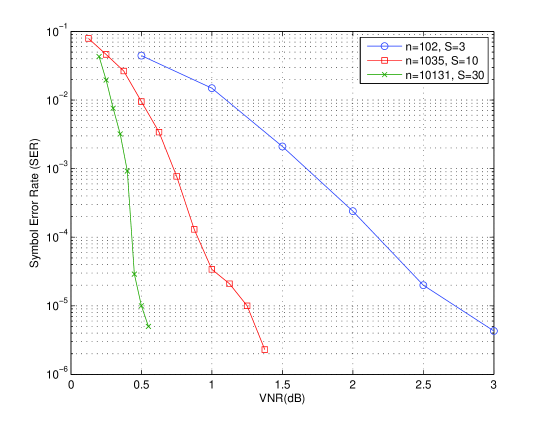
Figure 1: Comparison graph for various lengths of a turbo lattice.

The multi-stage decoding algorithm may not be the best choice here. Some other options are listed in the following paragraphs.

First, for low dimensional lattices a universal lattice code decoder [32] can be employed to decode turbo lattices. In that case, one can carve good lattice constellations from turbo lattices by choosing appropriate shaping regions [6].

Second, it is well-known that turbo codes can be considered as a class of graph-based codes on iterative decoding [33]. Also Tanner graph realization of lattices are introduced in [3]. In fact in a multi-stage decoding, after a “coarse” code is decoded, it is frozen and the decision is passed to a “fine” code. In other words, there is no iterative decoding across layers. If the nested underlying turbo codes of a turbo lattice are expressed as a Tanner-graph model as in [33] or the turbo lattice itself is presented by a Tanner-graph as in [3], then it seems feasible to do iterative decoding across layers, which may potentially increase the performance. However we should again be careful about short cycles in the corresponding Tanner-graph of turbo lattices as well as cycle-free lattices [23].

Third, lattice basis reduction algorithms and the faster version of that which works in complex plane [14] can also be employed to find closest lattice point to a received vector.

VII Simulation Results for Performance of Turbo Lattices

All simulation results presented are achieved using an AWGN channel, systematic recursive convolutional codes in the parallel concatenated scheme, and iterative turbo lattice decoder all discussed earlier. Indeed, we investigate turbo lattice designed using two identical terminated convolutional codes with generator matrix ${\bf G}_{A}(x)$. Turbo lattices of different lengths are examined. Furthermore, the performance of these turbo lattices are evaluated using BCJR algorithms [19] as constituent decoders for the iterative turbo decoder. Moreover, $S$-random interleavers of sizes $2^{5}$, $7^{3}$ and $15^{3}$ such that $S$ equals to $3$, $10$ and $30$ have been used, respectively. These results in turbo lattices of dimensions $(2^{5}+2)*3=102$, $(7^{3}+2)*3=1035$ and $(15^{3}+2)*3=10131$. The number of iterations for the iterative turbo decoder is fixed. It is equal to ten in all cases. Fig. 1 shows a comparison between turbo lattices formed with turbo codes of different lengths. These turbo lattices achieve a symbol error rate (SER) of $10^{-5}$ at an $\alpha^{2}=2.75~{}\mbox{dB}$ for size $102$, an $\alpha^{2}=1.25~{}\mbox{dB}$ for frame length $1035$. Also an SER of $10^{-5}$ is attained at an $\alpha^{2}=.5~{}\mbox{dB}$ for size $10131$.

In the following we compare these results for turbo lattices with other newly introduced latices including LDPC lattices [21] and LDLC lattices [28]. The comparison is presented in Table I.

Lattice	$n$	Error Probability	Distance from Capacity
LDPC Lattice	$2000$	NEP$=10^{-5}$	$2.8$ dB
LDLC Lattice	$1000$	SER$=10^{-5}$	$1.5$ dB
Turbo Lattice	$1035$	SER$=10^{-5}$	$1.25$ dB

TABLE I: A comparison between well-known and newly introduced lattices.

In Fig. 3 and for turbo lattices of sizes $n=102,~{}1035,~{}10131$, at SER of $10^{-5}$, we achieve $\alpha^{2}=2.75,~{}1.25$ and $.5$ dB away from capacity while for $n=100,~{}1000,~{}10000,~{}100000$, LDLC lattices [28] can work as close as $3.7,~{}1.5,~{}0.8$ and $0.6$ dB from capacity, respectively. Thus, we have an excellent performance of turbo lattices when compared with other lattices.

VIII Conclusion and Further Research Topics

The concept of turbo lattices is established using Construction D method for lattices along with a set of newly introduced nested turbo codes. To this end, tail-biting and terminated convolutional codes are concatenated in parallel. This parallel concatenation to induce turbo codes was supported with nested $S$-random interleavers. This gives us the possibility to combine the characteristics of convolutional codes and block codes to produce good turbo lattices. The fundamental parameters of turbo lattices for investigating the error performance are provided. This includes minimum distance, coding gain, kissing number and an upper bound on the probability of error. Finally, our experimental results show excellent performances for turbo lattices as expected by the theoretical results. More precisely, for example at SER of $10^{-5}$ and for $n=10131$ we can work as close as $\alpha^{2}=0.5$ dB from capacity.

Analyzing other factors and parameters of $b$-branches turbo lattices such as sphere packing, covering and quantization problem is also of great interest. Another interesting research problem is to find the error performance of turbo lattices designed by other types of interleavers including deterministic interleavers [26, 33].

Since the performance of turbo lattices depends on the performance of their underlying codes, then search for other well-behaved turbo-like codes would be interesting.

[A:Proofs] Theorem 2:

• Let ${\bf c}^{\ell}$ be a codeword with minimum weight in $\mathcal{C}_{\ell}$ for $1\leq\ell\leq a$. There exist $\beta_{j}^{({\ell})}\in\{0,1\}$ such that ${\bf c}^{\ell}=\sum_{j=1}^{k_{\ell}}\beta_{j}^{({\ell})}{\bf c}_{j}$. Since $\frac{1}{2^{{\ell}-1}}{\bf c}^{\ell}$ is in the form of (8), it belongs to $\Lambda$. Thus, we have

  $$d_{\min}(\Lambda)\leq\left\|\frac{1}{2^{{\ell}-1}}{\bf c}^{\ell}\right\|^{1/2}=\frac{1}{2^{{\ell}-1}}\sqrt{d_{\min}^{(\ell)}}.$$

  This means that $d_{\min}(\Lambda)\leq\min_{1\leq{\ell}\leq a}\left\{2,\frac{1}{2^{{\ell}-1}}\sqrt{d_{\min}^{(\ell)}}\right\}$. On the other hand the number $2$ in this formula happens when $\beta_{j}^{(\ell)}=0$ for all $j$ and $\ell$ and ${\bf z}=(0,\ldots,0,2,0,\ldots,0)$. Now, we set $L_{0}=(2\mathbb{Z})^{n}$ and

  $$L_{\ell}=\left\{{\bf x}+\sum_{j=1}^{k_{\ell}}\beta_{j}^{({\ell})}\frac{{\bf c}_{j}}{2^{{\ell}-1}}\right\}$$

  where $\beta_{j}^{({\ell})}=0$ or $1$ and ${\bf x}\in L_{{\ell}-1}$. Hence, $L_{a}=\Lambda$. It is easy to check that $L_{\ell}$ is a lattice. Let $0\neq{\bf v}$ be a vector of level ${\ell}$. If ${\ell}=0$ then $\|{\bf v}\|=4$. If ${\ell}>0$ then according to the definition of $L_{\ell}$ we can write ${\bf v}={\bf x}+{\bf y}$ where ${\bf x}\in L_{{\ell}-1}$ and ${\bf y}\in L_{\ell}$. The vector ${\bf y}$ has at least $d_{\min}^{(\ell)}$ components since it is in level ${\ell}$. It means that the norm of the vector ${\bf y}$ is at least $\frac{d_{\min}^{(\ell)}}{4^{{\ell}-1}}$. So ${\bf y}$ has at least $d_{\min}^{\ell}$ components equaling to $(1/2)^{\ell-1}$. Note also that every component in ${\bf x}$ is a multiple of $(1/2)^{\ell-2}$. Hence ${\bf v}$ has at least $d_{\min}^{\ell}$ components whose absolute values are no less than $(1/2)^{\ell-1}$. It follows that the norm of the vector ${\bf v}$ is at least $\frac{d_{\min}^{(\ell)}}{4^{{\ell}-1}}$ Thus, $d_{\min}(\Lambda)\geq\min_{1\leq{\ell}\leq a}\left\{2,\frac{1}{2^{{\ell}-1}}\sqrt{d_{\min}^{(\ell)}}\right\}$.

• The only points in $\Lambda$ that achieve $d_{\min}(\Lambda)$ are the $2n$ points $\pm 2{\bf e_{i}}$ for $1\leq i\leq n$ where ${\bf e_{i}}$ is the $i$–th unit vector plus the points which are in $\mathcal{C}_{\ell}$’s satisfying (11) for $1\leq{\ell}\leq a$. In other words when we have $d_{\min}^{2}(\Lambda)=\frac{d_{\min}^{(\ell)}}{4^{\ell-1}}$ for some $1\leq{\ell}\leq a$, then $4\geq\frac{d_{\min}^{(\ell)}}{4^{\ell-1}}$ and the codewords with minimum weight in $\mathcal{C}_{\ell}$ are the candidates to produce spheres which can touch the sphere with center $0$ and radius $\frac{d_{\min}(\Lambda)}{2}$. Therefore, these points must be in $\mathcal{C}_{\ell}$ with weight $d_{\min}^{(\ell)}$ such that $d_{\min}^{(\ell)}\leq 4^{{\ell}}$. It means that the kissing number of $\Lambda$ is upper bounded by

  $$~{}2n+\sum_{\begin{subarray}{c}1\leq{\ell}\leq a\\ d_{\min}^{(\ell)}\leq 4^{\ell}\end{subarray}}2^{d_{\min}^{(\ell)}}A_{d_{\min}^{(\ell)}}.$$ (25)

  The coefficient $2^{d_{\min}^{(\ell)}}$ appears since the nonzero entries of each lattice vector of $\Lambda$ can be positive or negative. We note that if $d_{\min}^{(\ell)}>4^{{\ell}}$, then the right hand side of (11) is equal to $2$ and the summations in (12) and (25) disappear.

Theorem 3: The vector

$$(0,\ldots,0,1,0,\ldots,0,f_{i,K+1}(x),\ldots,f_{i,N}(x))$$

is in the code if and only if there exists a polynomial $t_{i}(x)$ such that

$$t_{i}(x)\left(0,\ldots,0,r_{i}(x),0,\ldots,0,q_{i,K+1}(x),\ldots,q_{i,N}(x)\right)\equiv$$

$$(0,\ldots,0,1,\ldots,0,f_{i,K+1}(x),\ldots,f_{i,N}(x))\!\!\!\!\pmod{x^{L}-1}.$$

This happens if and only if every $r_{i}(x)$ has an inverse $\mbox{mod}~{}(x^{L}-1)$ and $q_{i,j}(x)\equiv f_{i,j}(x)r_{i}(x)\pmod{x^{L}-1}$ for $1\leq i\leq K$ and $K+1\leq j\leq N$ because $r_{i}^{-1}(x)=t_{i}(x)$ for $1\leq i\leq K$.

Proposition 4: Since the characteristic polynomial of the matrix ${\bf A}$ is $r(x)$, we conclude that $p({\bf A})=0$. We have that $\gcd(r(x),x^{L}-1)=1$ if and only if there exist two polynomials $s(x)$ and $t(x)$ such that $s(x)r(x)+t(x)(x^{L}-1)=1$. Put $x={\bf A}$, we get $t({\bf A})({\bf A}^{L}-{\bf I}_{m})={\bf I}_{m}$. Hence, we have $\det\left({\bf A}^{L}-{\bf I}_{m}\right)\neq 0$ if and only if $\gcd(r(x),x^{L}-1)=1$.

Theorem 9: Let $R_{\ell}^{0}=\frac{k_{\ell}^{0}}{n_{\ell}^{0}}$ denote the rate of the ${\ell}$–th component of the nested turbo codes when we scale $L$ and $k_{\ell}$’s by a factor of $t$. Then, we have

$$R_{\ell}^{0}=\frac{k_{\ell}^{0}}{n_{\ell}^{0}}=\frac{tk_{\ell}}{(2(Lt)N-(Lt)K)}=R_{\ell}.$$

We observe that in this case the interleaver size is $k^{0}=tk=(Lt)K$ and the interleaver $\Pi$ is a $(tk_{a},\ldots,tk_{1})$-nested interleaver. Also this is true for the actual rate of our nested turbo codes. Suppose $n_{\ell}^{0},k_{\ell}^{0}$ and $R_{\ell}^{0}$ be as above, then

$$R_{\ell}^{0} = \frac{k_{\ell}^{0}}{n_{\ell}^{0}-k^{0}+k_{\ell}^{0}}=\frac{tk_{\ell}}{(2(Lt)N-(Lt)K)-tk+tk_{\ell}}$$

$$= \frac{k_{\ell}}{n-k+k_{\ell}}=R_{\ell}.$$

Theorem 13: By using Theorem 2 and the paragraph above that, we easily get (20) and (22). For the coding gain we have

$$\gamma(\Lambda_{\mathcal{TC}}) = \frac{d^{2}_{\min}(\Lambda_{\mathcal{TC}})}{\det(\Lambda_{\mathcal{TC}})^{2/n}}=\frac{\min_{1\leq{\ell}\leq a}\left\{4,\frac{d_{\min}^{(\ell)}}{4^{{\ell}-1}}\right\}}{\left(2^{n-\sum_{{\ell}=1}^{a}k_{\ell}}\right)^{2/n}}$$

$$= 4^{\left(\sum_{{\ell}=1}^{a}R_{\ell}\right)-1}\min_{1\leq{\ell}\leq a}\left\{4,\frac{d_{\min}^{(\ell)}}{4^{{\ell}-1}}\right\}.$$

Theorem 15: Based on Equations (11) and (23), and the fact that $d_{\min}^{2}(2^{a-1}\Lambda_{\mathcal{TC}})=4^{a-1}d^{2}_{\min}(\Lambda_{\mathcal{TC}})$, we get

$$d_{\min}^{2}(\Lambda_{0})=4^{a-1}\min_{1\leq{\ell}\leq a}\left\{4,\frac{d_{\min}^{(\ell)}}{4^{{\ell}-1}}\right\}.$$

In addition, based on the geometric uniformity of lattices, it suffices to consider $\tilde{{\bf x}}=\tilde{{\bf y}}={\bf 0}$. Therefore, we have to prove that if $\|{\bf r}_{a}\|^{2}<d_{\min}^{2}(\Lambda_{0})/4$, then ${\bf r}_{a}$ will be decoded to ${\bf 0}$. There is an error in step ${\ell}$ if ${\bf x}_{{\ell}}\neq 0$, $1\leq{\ell}\leq a$. Assume that there have been no errors at the former steps $1\leq{\ell}^{\prime}<{\ell}$. Then in the ${\ell}$–th step we have ${\bf r}_{a-{\ell}+1}=\frac{{\bf r}_{a}}{2^{\ell-1}}$. Hence,

$$\|{\bf r}_{a-{\ell}+1}\|^{2}=\frac{1}{4^{{\ell}-1}}\|{\bf r}_{a}\|^{2}\leq\frac{d_{\min}^{2}(\Lambda_{0})}{4^{\ell}}$$

$$\leq 4^{a-1}\frac{d_{\min}^{(a-{\ell}+1)}}{(4^{a-{\ell}})(4^{\ell})}=\frac{d_{\min}^{(a-{\ell}+1)}}{4}.$$

This means that the largest sphere that can be inscribed in the Voronoi region associated with the lattice vector ${\bf 0}$ has radius $\frac{d_{\min}^{(a-{\ell}+1)}}{4}$. Since $\|{\bf r}_{a-{\ell}+1}\|^{2}<\frac{d_{\min}^{(a-{\ell}+1)}}{4}$, the point ${\bf r}_{a-{\ell}+1}$ is in the sphere of lattice $\Lambda_{a-{\ell}+1}=\mathcal{C}_{a-{\ell}+1}+2(\mathbb{Z})^{n}$, and thus no error can occur at step ${\ell}$.

References

- [1] I-B. Baik and S-Y. Chung, “Irregular low-density parity-check lattices,” in Proc. IEEE International Symposium on Information Theory, ISIT 2008, Toronto, Canada, pp. 2479–2483, 2008.
- [2] A.H. Banihashemi and I.F. Blake, “Trellis complexity and minimal trellis diagrams of lattices,” IEEE Trans. on Inform. Theory, vol. 44, pp. 1829–1847, 1998.
- [3] A.H. Banihashemi and F.R. Kschischang, “Tanner graphs for block codes and lattices: construction and complexity,” IEEE Trans. Inform. Theory, vol. 47, pp. 822–834, 2001.
- [4] E.S. Barnes and N.J.A. Sloane, “New lattice packings of spheres,” Canadian Journal of Mathematics, vol. 35, pp. 117–130, 1983.
- [5] C. Berrou, A. Glavieux, and P. Thitimajshima, “Near Shannon limit error-correcting coding and decoding: turbo codes,” in Proc. International Conference on Communications, pp. 1064–1070, 1993.
- [6] J. Boutros, E. Viterbo, C. Rastello, and J.C. Belfiore, “Good lattice constellations for both Rayleigh fading and Gaussian channels,” IEEE Trans. Inform. Theory, vol. 42, pp. 502–518, 1996.
- [7] J. Boutros and G. Zemor, “On quasi-cyclic interleavers for parallel turbo codes,” IEEE Trans. Inform. Theory, vol. 52, pp. 1732–1739, 2006.
- [8] M. Breiling, “A logarithmic upper bound on the minimum distance of turbo codes,” IEEE Trans. Inform. Theory, vol. 50, pp. 1692–1710, 2004.
- [9] Y-S. Choi, I-J. Baik, and S-Y. Chung, “Iterative decoding for low-density parity-check lattices,” in Proc. ICACT, pp. 358–361, 2008.
- [10] J.H. Conway and N.J.A. Sloane, “Sphere Packing, Lattices and Groups,” 3rd ed., New York, Springer-Verlag, 1998.
- [11] G.D. Forney, Jr., “A bounded distance decoding algorithm for the Leech lattices, with generalization,” IEEE Trans. Inform. Theory, vol. 35, pp. 906–909, 1989.
- [12] G.D. Forney Jr., M.D. Trott, and S-Y. Chung, “Sphere-bound-achieving coset codes and multilevel coset codes,” IEEE Trans. Inform. Theory, vol. 46, pp. 820–850, 2000.
- [13] G.D. Forney, Jr. and G. Ungerboeck, “Modulation and coding for linear gaussian channels”, IEEE Trans. Inform. Theory, vol. 44, pp. 2384–2415, 1998.
- [14] Y.H. Gan, C. Ling, and W.H. Mo, “Complex lattice reduction algorithm for low-complexity full-diversity MIMO detection,” IEEE Trans. Signal Processing, vol. 57, pp. 2701–2710, 2009.
- [15] J. Hokfelt, O. Edfors, and T. Maseng, “On the theory and performance of trellis termination methods for turbo codes,” IEEE J. Select. Areas Commun., vol. 19, pp. 838–847, 2001.
- [16] J. Harshan, E. Viterbo, and J.C. Belfiore, “Practical Encoders and Decoders for Euclidean Codes from Barnes-Wall Lattices,” submitted to IEEE Trans. Inform. Theory, arXiv:1203.3282v2.
- [17] H. Jin and J. McEliece, “Coding theorems for turbo code ensembles,” IEEE Trans. Inform. Theory, vol. 48, pp. 1451–1461, 2002.
- [18] N. Kahale and R. Urbanke, “On the minimum distance of parallel and serially concatenated codes,” in Proc. International Symposioum on Information Theory, ISIT 1998, Cambricge, MA, USA, 1998.
- [19] S. Lin and D.J. Costello, “Error Contorol Coding, Fundamentals and Application,” 2nd ed., New Jeresy, Pearson Prentice Hall, 2003.
- [20] G. Poltyrev, “On coding without restrictions for the AWGN channel,” IEEE Trans. Inform. Theory, vol. 40, pp. 409–417, 1994.
- [21] M.-R. Sadeghi, A.H. Banihashemi, and D. Panario, “Low density parity check lattices: construction and decoding analysis,” IEEE Trans. Inform. Theory, vol. 52, pp. 4481–4495, 2006.
- [22] M.-R. Sadeghi and D. Panario, “Low-density parity-check lattices based on Construction D’ and cycle-free Tanner Graph,” DIMACS 2003, vol. 68, pp. 86–90, 2003.
- [23] A. Sakzad and M.-R. Sadeghi, “On cycle-free lattices with high rate label codes,” Advances in Mathematics of Communications, vol. 4, pp. 441–452, 2010.
- [24] A. Sakzad, M.-R. Sadeghi, and D. Panario, “Cycle Structure of Permutation Functions over Finite Fields and their Applications,” to appear in Advances in Mathematics of Communications.
- [25] A. Sakzad, M.-R. Sadeghi, and D. Panario, “Construction of turbo lattices,” in Proc. 48th Annual Allerton Conference on Communication, Control, and Computing, Allerton, Chicago, USA, pp. 14–21, 2010.
- [26] A. Sakzad, D. Panario, M-R. Sadeghi, and N. Eshghi, “Self-inverse interleavers based on permutation functions for turbo codes,” in Proc. 48th Annual Allerton Conference on Communication, Control, and Computing, Allerton, Chicago, USA, pp. 22–28, 2010.
- [27] G. Solomon and H.C.A. van Tilborg, “A connection between block and convolutional codes,” SIAM J. Appl. Math., vol. 37, pp. 358–369, 1979.
- [28] N. Sommer, M. Feder, and O. Shalvi, “Low-density lattice codes,” IEEE Trans. Inform. Theory, vol. 54, pp. 1561–1586, 2008.
- [29] P. Stahl, J.B. Anderson, and R. Johannesson, “A note on tail-biting codes and their feed-back encoders,” IEEE Trans. Inform. Theory, vol. 48, pp. 529–534, 2002.
- [30] J. Sun and O.Y. Takeshita, “Interleavers for Turbo codes using permutation polynomials over integer rings,” IEEE Trans. Inform. Theory, vol. 51, no. 1, pp. 101–119, 2005.
- [31] V. Tarokh, A. Vardy, and K. Zeger, “Universal bound on the performance of lattice codes,” IEEE Trans. Inform. Theory, vol. 45, pp. 670–682, 1999.
- [32] E. Viterbo, and J. Boutros, “A universal lattice code decoder for fading channels,” IEEE Trans. Inform. Theory, vol. 45, pp. 1639–1642, 1999.
- [33] B. Vucetic, Y. Li, L.C. Perez, and F. Jiang, “Recent advances in turbo code design and theory,” Proceedings of the IEEE, Vol. 95, pp. 1323–1344, 2007.
- [34] C. Weis, C. Bettsteter, and S. Riedel, “Code construction and decoding of parallel concatenated tail-biting codes,” IEEE Trans. Inform. Theory, vol. 47, pp. 366–386, 2001.