A uniform version of the Petrov-Khovanskii theorem

Abstract.

An Abelian integral is the integral over the level curves of a Hamiltonian $H$ of an algebraic form $\omega$. The infinitesimal Hilbert sixteenth problem calls for the study of the number of zeros of Abelian integrals in terms of the degrees $H$ and $\omega$. Petrov and Khovanskii have shown that this number grows at most linearly with the degree of $\omega$, but gave a purely existential bound. Binyamini, Novikov and Yakovenko have given an explicit bound growing doubly-exponentially with the degree.

We combine the techniques used in the proofs of these two results, to obtain an explicit bound on the number of zeros of Abelian integrals growing linearly with $\deg\omega$.

1. Introduction

Let $H$ be a real bivariate polynomial and $\omega$ a one-form on ${\mathbb{R}}^{2}$. Let $\delta_{t}\subseteq\{H=t\}$ denote a continuous family of real ovals. Consider the Abelian integral

(1) $$I_{H,\omega}(t)=\int_{\delta_{t}}\omega$$

The infinitesimal Hilbert Sixteenth problem calls for the study of the zero set

(2) $$Z_{H,\omega}=\{t:I_{H,\omega}(t)=0\}.$$

In particular, the goal is to obtain an upper bound ${\mathcal{N}}(\deg H,\deg\omega)$ on $\#Z_{H,\omega}$ depending solely on the degrees of $H$ and $\omega$. Here and in the rest of the paper $\#A$ denotes the number of isolated points in the set $A$.

The infinitesimal Hilbert problem is motivated by the study of limit cycles born from the perturbation $\,\mathrm{d}H+\varepsilon\omega=0$ of the Hamiltonian system $\,\mathrm{d}H=0$. In particular, the existence of the uniform bound ${\mathcal{N}}(\deg H,\deg\omega)$ may be seen as a particular case of the general Hilbert sixteenth problem. We refer the reader to the surveys [3, 10] for further details and references.

1.1. Background

The first general result concerning the infinitesimal Hilbert problem was given in [8, 5]:

Theorem 1.

(3) $${\mathcal{N}}(n,m)<\infty$$

In other words, the number of zeros of Abelian integral is uniformly bounded in terms of the degrees of the Hamiltonian $H$ and the form $\omega$. However, this result is purely existential and does not give an explicit bound for ${\mathcal{N}}(n,m)$.

The following uniform upper bound, established in [1], constitutes an explicit solution for the infinitesimal Hilbert problem.

Theorem 2.

(4) $${\mathcal{N}}(n,n)\leqslant 2^{2^{\operatorname{\textup{Poly}}(n)}}$$

where $\operatorname{\textup{Poly}}(n)$ denotes an explicit polynomial of degree not exceeding 61.

We call the attention of the reader to the fact that the dependence of the upper bound (4) is doubly-exponential in both $\deg H$ and $\deg\omega$. In contrast, Petrov and Khovanskii proved the following result in an unpublished work (see [11, 7] for an exposition).

Theorem 3.

(5) $$\#Z_{H,\omega}\leqslant a(n)m+b(H)$$

where $n=\deg H,m=\deg\omega$, with $a(n)$ some explicit function and $b(H)$ some function of $H$ (for which a bound is not given).

The bound given by Theorem 3 is not uniform over the class of Hamiltonians of a given degree, due to the appearance of the term $B(H)$. However, using the methods developed in the proof of Theorem 1 it is possible to prove that this term is in fact uniformly bounded [11].

Theorem 4.

(6) $${\mathcal{N}}(n,m)\leqslant a(n)m+b(n)$$

where $n=\deg H,m=\deg\omega$, with $a(n)$ some explicit funcition and $b(n)$ some function of $n$ (for which a bound is not given).

In summary, Theorem 2 establishes an explicit bound on ${\mathcal{N}}(n,m)$ depending doubly-exponentially on $m$, whereas Theorem 4 establishes an existential bound depending linearly on $m$. The goal of this paper is to apply a combination of the ideas used in the proofs of these two results, to obtain an explicit bound depending linearly on $m$.

The result is as follows. We introduce the following notation to simplify the presentation of the results. We write $O^{+}(f(x))$ as a shorhand for $O(f(x)\log f(x))$. We write $\exp(x)$ for $2^{x}$, and $\exp^{+}(x)$ for $\exp(O^{+}(x))$. Finally we allow compositional iteration in the usual way, so $\exp^{2}(x)$ corresponds to $2^{2^{x}}$, etc.

Theorem 5.

(7) $${\mathcal{N}}(n,m)\leqslant\exp^{+2}(n^{2})\cdot m+\exp^{+5}(n^{2})$$

See subsection 5.3 for a discussion of the percise form of the bound and possible improvements.

2. Preliminaries and setup

In this section we review background from the theory of analytic differential equations, the theory of Abelian integrals, and the work [1].

2.1. Connections, integrability and regularity

Let $\Omega\in\operatorname{Mat}(\ell,\Lambda^{1}({\mathbb{C}}P^{m}))$ denote an $\ell\times\ell$ rational matrix one-form over ${\mathbb{C}}P^{m}$ with singular locus $\Sigma$. The form is said to be integrable if $\,\mathrm{d}\Omega=\Omega\wedge\Omega$. This condition is equivalent to the existence of a fundamental solution matrix $X(\cdot)$, defined over ${\mathbb{C}}P^{m}\setminus\Sigma$ and ramified over $\Sigma$, for the following system of equations

(8) $$\,\mathrm{d}X=\Omega\cdot X.$$

In other words, we view $\Omega$ as the matrix form of a connection defined on the trivial $\ell$-dimensional vector bundle over ${\mathbb{C}}P^{m}$ and $X$ as a fundamental matrix of horizontal sections.

Let $(\lambda_{1},\ldots,\lambda_{m})$ denote an affine chart on ${\mathbb{C}}P^{m}$, and for convenience of notation let $t=\lambda_{1},\lambda^{\prime}=(\lambda_{2},\ldots,\lambda_{m})$. Then the system (8) may be viewed as a family of linear systems of differential equations in the $t$ variable parameterized by $\lambda^{\prime}$,

(9) $$\frac{\,\mathrm{d}X}{\,\mathrm{d}t}=\Omega_{\lambda^{\prime}}(t)X(t).$$

We remark that not every system of the form (9) may be obtained in this manner. In particular, systems obtained in this manner are necessarily isomonodromic.

The system (8) is said to be regular if for any germ of a real analytic path $\gamma:({\mathbb{R}},0)\to{\mathbb{C}}P^{m}$ with $\gamma({\mathbb{R}}\setminus\{0\})\subseteq{\mathbb{C}}P^{m}\setminus\Sigma$, the rate of growth of the fundamental solution matrix along $\gamma$ is polynomial. Explicitly, we require that for suitable positive constants $c,k$ we have

(10) $$\left|X(\gamma(s))\right|^{\pm 1}\leqslant c\left|s\right|^{-k}\qquad\forall s\in({\mathbb{R}},0).$$

The analyticity of the curve $\gamma$ is required to rule out spiralling around the singular locus.

2.2. Monodromy and Quasi-Unipotence

To each closed loop $\gamma\in{\mathbb{C}}P^{m}\setminus\Sigma$ one may associate a continuation operator $\Delta_{\gamma}$ describing the result of analytic continuation of $X(\cdot)$ along $\gamma$. The monodromy matrix $M_{\gamma}\in\operatorname{GL}(\ell,{\mathbb{C}})$ is defined by the equation $\Delta_{\gamma}X=X\cdot M_{\gamma}$. It is clear that $M_{\gamma}$ depends only on the pointed homotopy class of $\gamma$, and that the conjugacy class of $M_{\gamma}$ depends only on the free homotopy class of $\gamma$. In the future we shall mainly be interested in the conjugacy class of the monodromy, and refer to the monodromy associated with a homotopy class of a closed loop in this sense.

A matrix $M$ is said to be quasi-unipotent if all of its eigenvalues are roots of unity. Equivalently, $M$ is quasi-unipotent if and only if there exist $j,k\in{\mathbb{N}}$ such that $(M^{j}-I)^{k}=0$, where $I$ denotes the identity matrix. We shall say that the monodromy along a loop $\gamma$ is quasi-unipotent if the associated monodromy matrix $M_{\gamma}$ is quasi-unipotent (note that this condition depends only on the conjugacy class of $M_{\gamma}$).

A loop $\gamma$ is said to be a small loop around $\lambda_{0}$ if there exists a germ of an analytic curve $\tau:({\mathbb{C}},0)\to({\mathbb{C}}P^{m},\lambda_{0})$ with $\tau({\mathbb{C}}\setminus\{0\})\subseteq{\mathbb{C}}\setminus\Sigma$ such that $\gamma$ is homotopic to a closed path $\tau(\{\left|z\right|=\varepsilon)$ for sufficiently small $\varepsilon$. We shall only be interested in the case $\lambda_{0}\in\Sigma$.

The system (8) is said to be quasiunipotent if the monodromy matrix associated to each small loop is quasi-unipotent. Note that this condition does not imply that every monodromy matrix associated with the system is quasi-unipotent. In particular, monodromies along loops encircling several singualities are often not small, and are not required to be quasi-unipotent (and this is indeed the case in natural examples).

2.3. Complexity of algebraic objects

In this subsection we give definitions for measuring the complexity of the formulas representing various algebraic objects. It is rather unusual in mathematics to be concerned with the particular formulas used for the description of an object. Questions of this form fall more neatly within the framework of mathematical logic. Indeed, strictly speaking the definitions in this subsection could be more accurately expressed in terms of logical formula complexity. In the interest of simplicity we content ourselves with simple algebraic approximations of these notions which are sufficient for our purposes.

We stress that all definitions in this subsection refer to a particular representation of a given object. For instance, $x^{2}/x$ and $x/1$ are viewed as distinct fractional representations of the same polynomial.

A polynomial $P\in{\mathbb{Z}}[x_{1},\ldots,x_{n}]$ is said to be a lattice polynomial. We shall say that such a polynomial is defined over ${\mathbb{Q}}$, if

(11) $$P(x_{1},\ldots,x_{n})=\sum_{\alpha}c_{\alpha}x^{\alpha}\qquad c_{\alpha}\in{\mathbb{Z}}$$

where $\alpha$ denotes a multiindex. We define the size of $P$ to be $\mathbf{S}\left(P\right)=\sum_{\alpha}\left|c_{\alpha}\right|$.

A rational function given by a fraction of the form $P/Q$ is said to be defined over ${\mathbb{Q}}$ if $P$ and $Q$ are defined over ${\mathbb{Q}}$. In this case, we define the size $\mathbf{S}\left(P/Q\right)$ to be $\mathbf{S}\left(P\right)+\mathbf{S}\left(Q\right)$.

Similarly, a one-form $\omega$ is said to be defined over ${\mathbb{Q}}$ if it is of the form

(12) $$\omega=\sum_{i}R_{i}(x)\,\mathrm{d}x_{i}$$

where $R_{i}$ are rational functions defined over ${\mathbb{Q}}$. In this case, we define the size $\mathbf{S}\left(\omega\right)$ to be $\sum_{i}\mathbf{S}\left(R_{i}\right)$.

Finally, say that a vector or a matrix is defined over ${\mathbb{Q}}$ if its of its components are, and define the size to be the sum of the sizes of components.

2.4. Counting zeros of multivalued vector functions

Recall that we may view the system (8) as a family of differential equations in the variable $t$, of the form (9). We shall be interested in studying the oscillatory behavior of the solutions of this equation. However, due to the fact that the solutions of (9) may be ramified, some care is required in measuring this oscillation.

Let $f$ be a (possibly multivalued) function defined in a domain $U\subseteq{\mathbb{C}}$. If $U$ is simply connected, then we define the following counting function as a measure for the number of zeros of $f$:

(13) $${\mathcal{N}}_{U}(f)=\sup_{b}\#\{t:b(t)=0\},$$

where $b$ varies over the branches of $f$ in $U$ (which are well defined univalued functions, since $U$ is simply connected).

For general domains, we use the following counting function,

(14) $${\mathcal{N}}_{U}(f)=\sup_{T\subseteq U}{\mathcal{N}}_{T}(f),$$

where $T$ varies over all triangular domains (i.e., domains whose boundary consists of straight line segment). The restriction on the geometry of $T$ is needed in order to avoid spiralling around a singular point. We stress that the closure of $T$ need not be contained in $U$. The boundary may contain singular points. When $U$ is omitted from the notation, it is understood to be the domain of analyticity of the function $f$.

Let $L$ be a linear space of (possibly multivalued) functions defined in a domain $U\subseteq{\mathbb{C}}$. As a measure for the number of zeros of an element of $L$, we use the following,

(15) $${\mathcal{N}}_{U}(L)=\sup_{f\in L}{\mathcal{N}}_{U}(f).$$

When $U$ is omitted from the notation, it is understood to be the common domain of analyticity of the elements of $L$.

Remark 1 (Semicontinuity).

As remarked in [1], the counting function ${\mathcal{N}}(\cdot)$ is lower semicontinuous with respect to the space $L$. In particular, if we have a family of spaces $L_{\nu}$ continuously depending on a paramter $\nu$, then an upper bound ${\mathcal{N}}(L_{\nu})<M$ for $\nu$ in a dense subset of the paramter space implies the same upper bound for every $\nu$.

We now consider the oscillations of vector-valued solutions of the system (9). Fix $\lambda^{\prime}$ such that the affine line $A={\mathbb{C}}P^{1}\times\{\lambda^{\prime}\}$ is not contained in $\Sigma$. Then $A$ intersects $\Sigma$ in finitely many points. Let $U$ denote the complement of this intsection.

Since the system (9) is non-singular in $U$, it admits an $\ell$-dimensional space $L_{\lambda^{\prime}}^{V}(\Omega)$ of (possibly multivalued) vector-valued solution functions. To measure the oscillation of these solutions, we shall consider the number of intersections of a solution with an arbitrary fixed linear hyperplane. Formally, we define the linear space

(16) $$L_{\lambda^{\prime}}(\Omega)=\{c\cdot f:c\in{\mathbb{C}}^{\ell},f\in L_{\lambda^{\prime}}^{V}\}$$

and the corresponding counting function

(17) $${\mathcal{N}}(\Omega)=\sup_{\lambda^{\prime}}{\mathcal{N}}(L_{\lambda^{\prime}}).$$

When the system $\Omega$ is clear from the context, we sometimes omit it from the notation and write $L_{\lambda}^{\prime}$.

We note that the counting function may in general be infinite. We also remark that by triangulation, one may use to counting function ${\mathcal{N}}(\cdot)$ to study the oscillation in more complicated domains.

2.5. Q-systems and Q-functions

In this subsection we introduce a class of systems of the form (8) for which explicit bounds on the counting function ${\mathcal{N}}(\Omega)$ may be derived. This class constitutes the main object of study of the paper [1].

Definition 2 (Q-System).

The system (8) is said to be an $(s,m,d,\ell$)-Q-system if $\Omega$ is an $\ell\times\ell$ matrix one-form defined over ${\mathbb{C}}P^{m}$ such that the following holds:

1. $\Omega$ is integrable.

2. $\Omega$ is regular.

3. $\Omega$ is quasi-unipotent.

4. $\Omega$ is defined over ${\mathbb{Q}}$, has size $s$, and coefficients of degree bounded by $d$.

Functions from the corresponding linear spaces $L_{\lambda^{\prime}}(\Omega)$ are said to be Q-functions.

The main interest in this class of systems stems from the following result of [1, Theoren 8], which plays the central role in the proof of Theorem 2.

Theorem 6.

Let $\Omega$ be an $(s,m,d,\ell)$-Q-system. Then we have the following explicit bound,

(18) $${\mathcal{N}}(\Omega)\leqslant s^{2^{\operatorname{\textup{Poly}}(m,d,\ell)}}$$

where $\operatorname{\textup{Poly}}(m,d,\ell)\leqslant O^{+}(d\ell^{4}m)^{5}$.

We will also require a result concerning the order of a Q-function near a singular point. Fix $\lambda^{\prime}$ and let $f(t)\in L_{\lambda^{\prime}}$ and $(t_{0},\lambda^{\prime})\in\Sigma$ a singular point of $\Omega$. Then, since $\Omega$ is regular and quasiunipotent, $f(t)$ admit an expansion

(19) $$f(t)=p(\ln(t-t_{0}))t^{\mu}+o(t^{\mu})\qquad p\in{\mathbb{C}}[v],\mu\in{\mathbb{R}}.$$

We call $\mu$ the order of $f$ at $t=t_{0}$, and denote $\mu=\operatorname{ord}_{t_{0}}f$. If $\gamma_{\varepsilon}$ denotes a circular arc of radius $\varepsilon$ and angle $\alpha$ around $t_{0}$, then

(20) $$\lim_{\varepsilon\to 0}\operatorname{Var}\operatorname{Arg}f(t)\big{|}_{\gamma_{\varepsilon}}=2\alpha\mu.$$

The following proposition follows in a straightforward manner from the proof of Theorem 6.

Proposition 3.

Let $\Omega$ be an $(s,m,d,\ell)$-Q-system. Fix some $(t_{0},\lambda^{\prime})\in\Sigma$ and let $f\in L_{\lambda^{\prime}}(\Omega)$. Then we have the following explicit bound,

(21) $$\left|\operatorname{ord}_{t_{0}}f\right|\leqslant s^{(d\ell)^{O(m)}}.$$

Proof.

By (20) it suffices to estimate the variation of argument of $f(t)$ along $\gamma_{\varepsilon}$ (in absolute value). We list the appropriate references to [1]. The estimate follows immediately from Principal Lemma 33 and Lemma 42, noting the the normalized length of $\gamma_{\varepsilon}$ approaches $2\pi$ as $\varepsilon\to 0$. We remark that the bound of Lemma 42 is stated for the variation of argument of $f$, but it in fact applies to the absolute value of the variation of argument as well (as is easily seen from the proof). ∎

2.6. Abelian integrals and the Gauss–Manin connection

In order to apply the theory of Q-systems, and in particular Theorem 6 to the study of Abelian integrals, it is necessary to produce a Q-system that they satisfy. The existence of such systems goes back to Picard–Fuchs (in the form (9)), and to Gauss–Manin (in the form (8)). Explicit derivations of this system (in the sense of subsection 2.3) were given in [6, 9]. For the convenience of the reader, we reproduce the relevant parts of the construction below. For proofs of all statements and further details see [1].

Let ${\mathcal{H}}_{n+1}$ denote the class of all Hamiltonians of degree $n+1$,

(22) $$H_{\lambda}(x_{1},x_{2})=\sum_{\left|\alpha\right|\leqslant n+1}\lambda_{\alpha}x^{\alpha}$$

where $\alpha$ is a 2-multiindex. Then $\lambda\in{\mathbb{C}}^{m}$ with $m=\frac{1}{2}(n+2)(n+3)$ provides an affine chart for ${\mathcal{H}}_{n+1}$. Let $\Gamma_{\lambda}$ denote the affine curve defined by the equation $H_{\lambda}=0$.

For generic $\lambda$, the rank of the first homology group $H_{1}(\Gamma_{\lambda},{\mathbb{Z}})$ is $\ell=n^{2}$. One may choose a set of generators for this group over a fixed generic fibre $\lambda=\lambda_{0}$, and transport them horizontally with respect to the Gauss–Manin connection to obtain sections $\delta_{1}(\lambda),\ldots,\delta_{\ell}(\lambda)$, ramified over a singular set $\Sigma^{*}\subset{\mathcal{H}}_{n}$. Under a further genericity assumption $\lambda\not\in\Sigma\supset\Sigma^{*}$, we may assume further that the first cohomology group $H^{1}(\Gamma_{\lambda},{\mathbb{C}})$ is generated by the monomial one-forms

(23) $$\omega_{\alpha}=x_{1}\cdot x^{\alpha}\,\mathrm{d}x_{2}\qquad 0\leqslant\alpha_{1},\alpha_{2}\leqslant n-1.$$

Definition 4.

The period matrix $X(\lambda)$ is the $\ell\times\ell$ matrix

(24) $$X(\lambda)=\begin{pmatrix}\int_{\delta_{1}(\lambda)}\omega_{1}&\cdots&\int_{\delta_{\ell}(\lambda)}\omega_{1}\\ \vdots&\ddots&\vdots\\ \int_{\delta_{1}(\lambda)}\omega_{\ell}&\cdots&\int_{\delta_{\ell}(\lambda)}\omega_{\ell}\end{pmatrix}$$

defined on ${\mathcal{H}}_{n+1}\setminus\Sigma$ and ramified over $\Sigma$.

The period matrix satisfies a system of differential equations known as the Picard–Fuchs system (or Gauss–Manin connection). The following resut shows that this system is in fact a Q-system.

Theorem 7.

The period matrix satisfies the equation $\,\mathrm{d}X=\Omega X$, where $\Omega$ is an $(s,m,d,\ell)$-Q-system with

(25) $$s\leqslant 2^{\operatorname{\textup{Poly}}(n)},\quad m\leqslant O(n^{2}),\quad d\leqslant O(n^{2}),\quad\ell=n^{2}.$$

2.7. Polynomial envelopes

Let $L$ be the linear space spanned by $r$ (possibly multivalued) functions $f_{1}(t),\ldots,f_{r}(t)$ defined on a domain $U\subset{\mathbb{C}}$. Denote by ${\mathcal{P}}^{k}$ the space of polynomials of degree at most $k$. By a slight abuse of notation, we also denote by ${\mathcal{P}}^{k}$ a $(k,1,1,k)$-Q-system such that the entries of its fundamental solution matrix span the space ${\mathcal{P}}^{k}$ (such a system may easily be constructed).

Definition 5.

The polynomial envelope of degree $k$ of the space $L$ is defined to be

(26) $${\mathcal{P}}^{k}\otimes L=\left\{\sum_{i=1}^{r}p_{i}(t)f_{i}(t)\right\},\qquad p_{i}\in{\mathbb{C}}[t],\deg p_{i}\leqslant k.$$

Similarly, the polynomial envelope of a Q-system $\Omega$ is defined to be ${\mathcal{P}}^{k}\otimes\Omega$ (the tensor product of Q-systems is discussed in section 4, Transformation 5).

To establish a link between the polynomial envelope and the study of Abelian integrals we require the following result [2, 4]. We use the notation of subsection 2.6.

Proposition 6.

For a generic Hamiltonian $H_{\lambda}$ and for every polynomial one-form $\omega$ there exist univariate polynomials $p_{\alpha}\in{\mathbb{C}}[t]$ and bivariate polynomials $u,v\in{\mathbb{C}}[x_{1},x_{2}]$ such that

(27) $$\omega=\sum_{\alpha}(p_{\alpha}\circ H_{\lambda})\cdot\omega_{\alpha}+u\,\mathrm{d}H_{\lambda}+\,\mathrm{d}v,\qquad 0\leqslant\alpha_{1,2}\leqslant n-1,$$

where

(28) $$\left\{\begin{array}[]{c}(n+1)\deg p_{\alpha}+\deg\omega_{\alpha}\\ \deg v\\ n+\deg u\\ \end{array}\right.\leqslant\deg\omega$$

Let $L_{\lambda}^{e}$ denote the linear space of Abelian integrals of forms of degree at most $e$ over the Hamiltonian $H_{\lambda}$, and let $L_{\lambda}^{B}$ denote the linear space of Abelian integrals of the basic forms $\omega_{\alpha}$.

Consider now an arbitrary polynomial one-form $\omega$ of degree at most $e$. Let $\delta\in H_{1}(\{H_{\lambda}=s\},{\mathbb{Z}})$ be a cycle on the $s$-level surface of $H_{\lambda}$. Then $H_{\lambda}\big{|}_{\delta}\equiv s$ and $\,\mathrm{d}H_{\lambda}\big{|}_{\delta}\equiv 0$. Integrating (27) over $\delta$,

(29) $$\int_{\delta}\omega=\sum_{\alpha}p_{\alpha}(s)\int_{\delta}w_{\alpha},\qquad\deg p_{\alpha}\leqslant\lceil e/(n+1)\rceil.$$

Corollary 7.

For a generic Hamiltonian $H_{\lambda}$,

(30) $$L_{\lambda}^{e}\subseteq{\mathcal{P}}^{\lceil e/(n+1)\rceil}\otimes L_{\lambda}^{B}.$$

In particular, at least when the Hamiltonian is generic, ${\mathcal{N}}(L_{\lambda}^{e})$ is majorated by ${\mathcal{N}}({\mathcal{P}}^{\lceil e/(n+1)\rceil}\otimes L_{\lambda}^{B})$.

3. Statement of the main result

In this section we present the main result of the paper and deduce a corollary concerning the zeros of Abelian integrals. We begin by stating the general result of Petrov-Khovanskii. Our statement differs slightly from the usual formulation in order to facilitate the analogy to the uniform case.

To simplify the notation, when speaking about an $(s,m,d,\ell)$-Q-system we denote by $\nu$ the number of singular points of the system. We record the following estimate,

(31) $$\nu\leqslant O(\ell^{2}d).$$

Indeed, each singular point must be a pole of one of the $\ell^{2}$ entries of $\Omega$, and by degree considerations each entry may admit at most $d$ poles.

Let $f_{1}(t),\ldots,f_{\ell}(t)$ be $\ell$ (possibly multivalued and singular) functions on ${\mathbb{C}}P^{1}$, and let $L_{f}$ denote the linear space they span. Denote by $X_{f}$ the matrix

(32) $$X_{f}=\begin{pmatrix}f_{1}(t)&\cdots&f_{\ell}(t)\\ f^{\prime}_{1}(t)&\cdots&f^{\prime}_{\ell}(t)\\ &\vdots&\\ f^{(\ell)}_{1}(t)&\cdots&f^{(\ell)}_{\ell}(t)\end{pmatrix}.$$

Suppose that $\Omega_{f}=\,\mathrm{d}X_{f}\cdot X_{f}^{-1}$ is a rational matrix function of degree $d$ which is regular and quasiunipotent.

The following result can essentially be proved by combining the proofs of the Petrov-Khovanskii and the Varchenko-Khovanskii theorems (see [11]).

Theorem 8.

Under the conditions of the paragraph above,

(33) $${\mathcal{N}}({\mathcal{P}}^{k}\otimes\Omega_{f})\leqslant\frac{(2\nu)^{2^{\nu+1}\ell^{2}}-1}{2\nu-1}k+C\qquad\forall k\in{\mathbb{N}},$$

where $C$ is a constant depending only on $\Omega_{f}$ (for which a bound is not given). In particular, the number of zeros of a function in the $k$-th polynomial envelope of $L_{f}$ grows at most linearly with $k$.

The Petrov-Khovanskii result for Abelian integrals, Theorem 3, follows from Theorem 8 and Corollary 7 for generic Hamiltonians. A slightly more refined argument is needed in order to remove the genericity assumption. We exclude this argument from our presentation, as we shall soon see that our uniform version of the bound immediately extends from the generic case to the singular case.

We note that the system $\Omega_{f}$ arising from the formulation of Theorem 8 satisfies the various conditions required for a Q-system, apart from the condition of being defined over ${\mathbb{Q}}$. This is not a coincidence. In fact, the condition of being defined over ${\mathbb{Q}}$ is percisely the condition responsible for the emergence of uniform bounds in the class of Q-systems.

We now state our main result.

Theorem 9.

Let $\Omega$ be an $(s,m,d,\ell)$-Q-system. Then

(34) $${\mathcal{N}}({\mathcal{P}}^{k}\otimes\Omega)\leqslant\frac{(3\nu)^{8^{\nu}\ell^{2}}-1}{3\nu-1}+s^{\exp^{+}(\exp^{+}(4^{4^{\nu}\ell^{2}})d^{5}m^{5})}$$

Note that, in contrast to Theorem 8, the bound in Theorem 9 is fully explicit. Also note that while Theorem 8 applies to a particular set of functions, Theorem 9 applies to families of functions depending (as Q-functions) on an arbitrary number of parameters $\lambda^{\prime}$, and the bound is uniform over the entire family.

Combining Theorem 9 with Corollary 7, we obtain an upper bound $\exp^{+2}(n^{2})\cdot m+\exp^{+5}(n^{2})$ for the number of zeros of an Abelian integral of degree $e$ over a generic Hamiltonian $H_{\lambda}$ of degree $n$. By the semicontinuity of the counting function ${\mathcal{N}}(\cdot)$ (see Remark 1) this bound extends over the entire class of Hamiltonians, thus proving Theorem 5.

We note here that the implication above is a generally useful aspect of the theory of Q-functions – uniform bounds extend directly from the generic case to degenerate cases. Approaches based on compactness arguments usually require a more detailed analysis of the behavior near the singular strata (see for instance the proof of Theorem 4 in [11]).

4. Transformations of Q-systems

The approach employed by Petrov and Khovanskii in the proof of Theorem 8 requires that we perform a number of transformations to the functions being considered. Our objective is to obtain uniform bounds by applying Theorem 6. It is therefore necessary to prove that the appropriate transformations can be carried it within the class of Q-systems. In this section we prove that this is indeed the case, and analyze the affect of each of the transformations on the parameters $(s,m,d,\ell)$.

Let $\Omega$ denote an $(s,m,d,\ell)$-Q-system, and let $X(\cdot)$ denote a fundamental solution for $\Omega$. We assume that the base of the system is ${\mathbb{C}}^{m}$, with an affine chart $\lambda=(t,\lambda^{\prime})$.

Transformation 1 (Shift).

There exists an $(\hat{s},\hat{m},\hat{d},\hat{\ell})$-Q-system $\hat{\Omega}$ defined over the base space ${\mathbb{C}}^{m}\times{\mathbb{C}}$, with affine chart $\lambda\times\mu$, whose fundamental solution $\hat{X}(\cdot)$ is given by

(35) $$\hat{X}(t,\lambda^{\prime},\mu)=X(t+\mu,\lambda^{\prime})$$

and

(36) $$\hat{s}=\operatorname{\textup{Poly}}(s,m,d,\ell),\quad\hat{m}=m+1,\quad\hat{d}=d,\quad\hat{\ell}=\ell$$

Proof.

Suppose that

(37) $$\Omega=\Omega_{t}(t,\lambda^{\prime})\,\mathrm{d}t+\Omega_{\lambda^{\prime}}(t,\lambda^{\prime})\,\mathrm{d}\lambda^{\prime}.$$

Then

(38) $$\hat{\Omega}=\Omega_{t}(t+\mu,\lambda^{\prime})(\,\mathrm{d}t+\,\mathrm{d}\mu)+\Omega_{\lambda^{\prime}}(t+\mu,\lambda^{\prime})\,\mathrm{d}\lambda^{\prime}.$$

Since $\hat{\Omega}$ has an explicit solution $\hat{X}(\cdot)$, it is clear that $\hat{\Omega}$ is integrable. It is also clear that the regularity and quasiunipotence of $\hat{X}(\cdot)$ follows from that of $X(\cdot)$.

For the complexity analysis, it remains only to notice that we increased the dimension of the base space by one, and that the complexity of the formula for $\hat{\Omega}$ is polynomial in the complexity and the maximal degree of the formula for $\Omega$, the dimension of $\Omega$ and the dimension of the base space. ∎

We remark that it is generally not possible to perform a shifting transformation by a specific fixed value $\mu_{0}$. Indeed, the formula for $\hat{\Omega}$ in this case would involve the specific value $\mu_{0}$ which may be irrational, while explicit algebraic formulas by our definitions may use only integer coefficients. We circumvent this difficulty by extending the parameter space of the system with an additional parameter $\mu$. Specific shifts of the system may be obtained by restricting $\mu$ to $\mu_{0}$. The crucial condition which allows this construction is that the system is not only a Q-system for the fixed value $\mu_{0}$, but rather it is a Q-system with respect to the free parameter $\mu$. This technique is generally useful in the study of Q-systems, and has already appeared in the context of the conformally invariant slope in [1].

We now consider the transformation of $\Omega$ that corresponds to folding the $t$-plane by the transformation $w=t^{2}$.

Transformation 2 (Fold).

There exists an $(\hat{s},\hat{m},\hat{d},\hat{\ell})$-Q-system $\hat{\Omega}$ defined over the base space ${\mathbb{C}}^{m}$ with affine chart $w\times\lambda^{\prime}$, whose fundamental solution $\hat{X}(\cdot)$ is given by

(39) $$\hat{X}(w,\lambda^{\prime})=X(t,\lambda^{\prime})\oplus\left(tX(t,\lambda^{\prime})\right)$$

where $w=t^{2}$, and

(40) $$\hat{s}=\operatorname{\textup{Poly}}(s,m,d,\ell),\quad\hat{m}=m,\quad\hat{d}=d+2,\quad\hat{\ell}=2\ell$$

Proof.

As in the proof of Transformation 1, it is clear that $\hat{\Omega}$ is integrable and regular. To prove quasi-unipotence, let $\gamma$ be a small loop in the $(w,\lambda^{\prime})$ space. If $\gamma$ loops around a point with $w\neq 0$ then it corresponds to a small loop in the $(t,\lambda^{\prime})$ plane, and the monodromy of $\hat{X}(w,\lambda^{\prime})=\operatorname{diag}(X(t,\lambda^{\prime}),tX(t,\lambda^{\prime}))$ around this loop is quasi-unipotent by the quasi-unipotence of $\Omega$. If $\gamma$ loops around a point with $w=0$ then $\gamma^{2}$ corresponds to a small loop in the $(t,\lambda^{\prime})$ plane, and by the same reasoning we deduce that $M_{\gamma^{2}}$, the monodromy of $\hat{X}(w,\lambda^{\prime})$ along $\gamma^{2}$, is quasi-unipotent. But $M_{\gamma^{2}}=M_{\gamma}^{2}$, and a matrix whose square is quasi-unipotent is itself quasi-unipotent. Thus $M_{\gamma}$ is quasi-unipotent as claimed.

To explicitly define $\hat{\Omega}$, suppose that

(41) $$\Omega=\Omega_{t}(t,\lambda^{\prime})\,\mathrm{d}t+\Omega_{\lambda^{\prime}}(t,\lambda^{\prime})\,\mathrm{d}\lambda^{\prime}.$$

Then we may write

(42) $$\hat{\Omega}(w,\lambda^{\prime})=\operatorname{diag}(\Omega_{t}(t,\lambda^{\prime})\,\mathrm{d}t+\Omega_{\lambda^{\prime}}(t,\lambda^{\prime})\,\mathrm{d}\lambda^{\prime},\Omega_{t}(t,\lambda^{\prime})\,\mathrm{d}t+\Omega_{\lambda^{\prime}}(t,\lambda^{\prime})\,\mathrm{d}\lambda^{\prime}).$$

Since $\,\mathrm{d}t=\,\mathrm{d}w/2t$ we may rewrite this expression in the form

(43) $$\hat{\Omega}(w,\lambda^{\prime})=\operatorname{diag}(\frac{\Omega_{t}(t,\lambda^{\prime})}{2t}\,\mathrm{d}w+\Omega_{\lambda^{\prime}}(t,\lambda^{\prime})\,\mathrm{d}\lambda^{\prime},\frac{\Omega_{t}(t,\lambda^{\prime})}{2t}\,\mathrm{d}w+\Omega_{\lambda^{\prime}}(t,\lambda^{\prime})\,\mathrm{d}\lambda^{\prime}).$$

We now replace each occurence of $t^{2}$ by $w$, giving an expression

(44) $$\hat{\Omega}(w,\lambda^{\prime})=\operatorname{diag}(\Omega_{0}(w,\lambda^{\prime})+t\Omega_{1}(w,\lambda^{\prime}),\Omega_{0}(w,\lambda^{\prime})+t\Omega_{1}(w,\lambda^{\prime})).$$

Finally, since the second block in $\hat{X}$ is equal to $t$ multiplied by the first block, we may rewrite this as

(45) $$\hat{\Omega}(w,\lambda^{\prime})=\operatorname{diag}(\Omega_{0}(w,\lambda^{\prime})+1/t^{2}\Omega_{1}(w,\lambda^{\prime}),\Omega_{1}(w,\lambda^{\prime})+\Omega_{0}(w,\lambda^{\prime})),$$

which is an explicit expression for $\hat{\Omega}$. It is clear that the complexity of this expression is polynomial in $s,m,d,\ell$, the base space dimension is unchanged, the dimension of $\hat{\Omega}$ is $2\ell$, and the maximal degree of the coefficients of $\hat{\Omega}$ is at most $d+2$. ∎

Remark 8.

If the singular points of $\Omega$ for a specific value of $\lambda^{\prime}$ form a set $\{s_{j}\}$, then the singular values of $\hat{\Omega}$ form the set $\{s_{j}^{2}\}\cup\{0,\infty\}$ since $0$ and $\infty$ are the two critical values of the folding map.

We next consider symmetrization of $\Omega$ around the real line. This transformation was analyzed in [1, 3.2]. We state here only the result and omit the proof (which is straightforward).

For convenience we introduce the following notation. The reflection of a function $f(t)$ along the real line is given by

(46) $$f^{\dagger}(t)=\overline{f(\overline{t})}.$$

If $f$ is multivalued then one may select an analytic germ of $f$ at some point on the real line, reflect this germ, and analytically continue the result. In cases where this choice is significant we shall state the point of reflection explicitly. We will also use the ${\dagger}$ notation for vector and matrix valued functions in the obvious way. In this paper the reflection is always taken with respect to the time variable $t$.

Transformation 3 (Symmetrization).

There exists an $(\hat{s},\hat{m},\hat{d},\hat{\ell})$-Q-system $\Omega^{\ominus}=\hat{\Omega}$ defined over the same base space as $\Omega$, whose fundamental solution $\hat{X}(\cdot)$ is given by

(47) $$\hat{X}(t,\lambda^{\prime})=X(t,\lambda^{\prime})\oplus X^{\dagger}(t,\lambda^{\prime}),$$

and

(48) $$\hat{s}=\operatorname{\textup{Poly}}(s,m,d,\ell),\quad\hat{m}=m,\quad\hat{d}=d,\quad\hat{\ell}=2\ell$$

Remark 9.

The key feature of the symmetrization transform is that the corresponding solution spaces $L_{\lambda^{\prime}}(\hat{\Omega})$ are closed under taking real and imaginary parts on the real line. Indeed, for any $f(t)\in L_{\lambda^{\prime}}(\hat{\Omega})$ we have also $f^{\dagger}(t)\in L_{\lambda^{\prime}}(\hat{\Omega})$, and therefore

(49) $$\operatorname{Re}f=\frac{1}{2}\left(f(t)+f^{\dagger}(t)\right)\in L_{\lambda^{\prime}}(\hat{\Omega})$$

(50) $$\operatorname{Im}f=\frac{1}{2i}\left(f(t)-f^{\dagger}(t)\right)\in L_{\lambda^{\prime}}(\hat{\Omega})$$

For completeness we also list the two canonical transformations of direct sum and tensor product. Here we let $\Omega_{i}$ denote an $(s_{i},m,d_{i},\ell_{i})$-Q-system with fundamental solution $X_{i}(\cdot)$ for $i=1,2$, defined over a common base space. We again omit the proofs (which are straightforward).

Transformation 4 (Direct Sum).

There exists an $(\hat{s},\hat{m},\hat{d},\hat{\ell})$-Q-system $\Omega_{1}\oplus\Omega_{2}$ defined over the same base space as $\Omega_{1,2}$, whose fundamental solution is given by $X_{1}\oplus X_{2}$, and

(51) $$\hat{s}=s_{1}+s_{2},\quad\hat{m}=m,\quad\hat{d}=\max(d_{1},d_{2}),\quad\hat{\ell}=\ell_{1}+\ell_{2}$$

Transformation 5 (Tensor Product).

There exists an $(\hat{s},\hat{m},\hat{d},\hat{\ell})$-Q-system $\Omega_{1}\otimes\Omega_{2}$ defined over the same base space as $\Omega_{1,2}$, whose fundamental solution is given by $X_{1}\otimes X_{2}$, and

(52) $$\hat{s}=\operatorname{\textup{Poly}}(s_{1,2},m_{1,2},d_{1,2},\ell_{1,2}),\quad\hat{m}=m,\quad\hat{d}=\max(d_{1},d_{2}),\quad\hat{\ell}=\ell_{1}\ell_{2}$$

Remark 10.

Here we use $\otimes$ to denote the tensor product of $\Omega_{1,2}$ as connections, but in order to avoid confusion we note that the matrix form representing this connection is in fact $\left(\Omega_{1}\otimes I\right)\oplus\left(I\otimes\Omega_{2}\right)$.

5. Demonstration of the main result

In this section we present the demonstration of Theorem 9. The proof follows the same strategy as the Petrov-Khovanskii proof of Theorem 8. We first assume that all singular points of the system $\Omega$ are real. In this case it is possible to control the variation of argument by applying a clever inductive argument due to Petrov. For the general case, we show that the system may be transformed to a system with real singular points, and invoke the preceding case.

Recall that we denote by $L_{\lambda}^{\prime}$ the space of all linear combinations of solutions of the system $\Omega$ for a fixed value $\lambda^{\prime}$, viewed as functions of $t$ (see (16)).

5.1. The case of real singular points

In this subsection we assume that all singular points of $\Omega$ are real.

Proposition 11.

Let $\Omega$ be an $(s,m,d,\ell)$-Q-system, and let $\lambda^{\prime}$ be a paramter such that the singular locus of the system $\Omega_{\lambda^{\prime}}$ is contained in ${\mathbb{R}}$. Let $r,k\in{\mathbb{N}}$ and denote

(53) $$f(t)=\sum_{i=1}^{r}p_{i}(t)f_{i}(t)\qquad\forall i\left\{\begin{array}[]{cc}p_{i}(t)\in{\mathbb{R}}[t]\\ \deg p_{i}(t)\leqslant k\\ f_{i}\in L_{\lambda^{\prime}}\end{array}\right.$$

Finally, recall that we denote by $\nu$ the number of singular points of $\Omega$. Then

(54) $${\mathcal{N}}(f)\leqslant\frac{\nu^{r}-1}{\nu-1}k+s^{\alpha(m,d,\ell,r)},\qquad\alpha(m,d,\ell,r)=\exp^{+}(8^{r}\ell^{5\cdot 2^{r+1}}d^{5}m^{5})$$

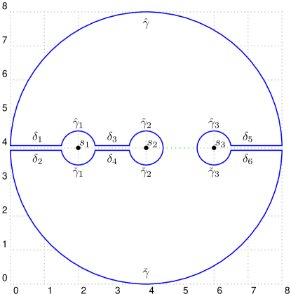
Figure 1. Contour of integration

Proof.

Let the domain $U$ and its boundary $\Gamma$, partitioned as the union of the curves $\delta_{i},\hat{\gamma}_{i},\check{\gamma}_{i},\hat{\gamma},\check{\gamma}$, be as indicated in figure 1 where the radius of each $\gamma_{i}$ (resp. $\gamma$) may be arbitrarily small (resp. large). Notice that one segment of the real domain is in fact contained in $U$ (indicated by a dotted line in the figure). Since any triangle avoiding the singular points can intersect at most one such segment, and since we can select $U$ to contain any single segment, it follows that to bound ${\mathcal{N}}(f)$ it will suffice to bound ${\mathcal{N}}_{U}(f)$ independently of the radii defining $U$. We proceed by induction on $r$.

When $r=1$, we have $f(t)=p_{1}(t)f_{1}(t)$. Thus by Theorem 6

(55) $${\mathcal{N}}_{U}(f)\leqslant{\mathcal{N}}_{U}(f_{1})+k\leqslant C_{1}+k$$

where

(56) $$C_{1}=s^{\exp^{+}((d\ell^{4}m)^{5})},$$

giving the desired conclusion.

For arbitrary $r$, we proceed by applying the argument principle. We first rewrite $f(t)$ as

(57) $$f(t)=\sum_{i=1}^{r}p_{i}(t)f_{i}(t)=f_{1}(t)F(t)$$

where

(58) $$F(t) =p_{1}(t)+\sum_{i=2}^{r}p_{i}(t)\frac{f_{i}(t)}{f_{1}(t)}$$

(59) $$=p_{1}(t)+\left|f_{1}(t)\right|^{-2}\sum_{i=2}^{r}p_{i}(t)f_{i}(t)\overline{f_{1}(t)}.$$

By Theorem 6 and the argument principle,

(60) $${\mathcal{N}}_{U}(f)={\mathcal{N}}_{U}(f_{1})+{\mathcal{N}}_{U}(F)\leqslant C_{1}+(2\pi)^{-1}\operatorname{Var}\operatorname{Arg}F(t)\big{|}_{\Gamma}.$$

We consider the variation of argument on each piece of $\Gamma$ separately.

The arcs $\hat{\gamma}_{i},\check{\gamma}_{i}$ are traversed in reverse orientation. Therefore we need to bound the variation of argument along these arcs from below. By (20) the contribution of each arc approaches $\pi\operatorname{ord}F\big{|}_{t=s_{i}}$ as $\varepsilon\to 0$. By Proposition 3, the order of each $f_{i}$ is bounded in absolute value by

(61) $$C_{2}=s^{(d\ell)^{O(m)}}.$$

Using (58) we deduce that $\operatorname{ord}F\big{|}_{t=s_{i}}\geqslant-2C_{2}$. Therefore

(62) $$\operatorname{Var}\operatorname{Arg}F(t)\big{|}_{\hat{\gamma}_{i},\check{\gamma}_{i}}\leqslant 2\pi C_{2}\qquad i=1,\ldots,\nu.$$

Similarly, the arcs $\hat{\gamma},\check{\gamma}$ may be seen as small circular arcs around the point at infinity. We argue as above, noting that in this case the order of each $p_{j}(t)$ is bounded from below by $-k$. It follows that $\operatorname{ord}F\big{|}_{t=\infty}\geqslant-2C_{2}-k$. Therefore

(63) $$\operatorname{Var}\operatorname{Arg}F(t)\big{|}_{\hat{\gamma},\check{\gamma}}\leqslant\pi(2C_{2}+k).$$

It remains to consider the variation of argument along the segments $\delta_{i}$. Assume that $F(t)$ is not purely real on $\delta_{i}$ (otherwise there is no variation of argument). The key observation is that

(64) $$\operatorname{Var}\operatorname{Arg}F(t)\big{|}_{\delta_{i}}\leqslant\pi({\mathcal{N}}_{\delta_{i}}\operatorname{Im}_{\delta_{i}}F(t)+1)$$

where $\operatorname{Im}_{\delta_{i}}$ denotes the imaginary part taken with respect to the segment $\delta_{i}$. This fact, known as “the Petrov trick”, is a simple topological consequence of the fact that the variation of argument of a curve contained in a half-plane is at most $\pi$.

Using (59) and noting that $p_{j}(t)$ is real on the real line for every $j$, we see that on $\delta_{i}$

(65) $$\begin{split}\operatorname{Im}_{\delta_{i}}F(t)&=\left|f_{1}(t)\right|^{-2}\sum_{i=2}^{r}p_{i}(t)\operatorname{Im}_{\delta_{i}}\left(f_{i}(t)\overline{f_{1}(t)}\right)\\ &=\left|f_{1}(t)\right|^{-2}G(t)\end{split}$$

where (taking reflection with respect to $\delta_{i}$),

(66) $$G(t)=\sum_{i=2}^{r}p_{i}(t)\operatorname{Im}_{\delta_{i}}\left(f_{i}(t)f^{\dagger}_{1}(t)\right).$$

We used the fact that $f(\overline{t})=f^{\dagger}(t)$ on $\delta_{i}$.

Let $\hat{\Omega}=\left(\Omega\otimes\Omega^{\ominus}\right)^{\ominus}$. Then $\hat{\Omega}$ is a $(\operatorname{\textup{Poly}}(s,m,d,\ell),m,d,4\ell^{2})$-Q-system, and

(67) $$\operatorname{Im}_{\delta_{i}}f_{i}(t)f^{\dagger}_{1}(t)\in L_{\lambda^{\prime}}(\hat{\Omega})\qquad i=2,\ldots,r.$$

Note that $\hat{\Omega}_{\lambda^{\prime}}$ has the same singularities as $\Omega_{\lambda^{\prime}}$, since the singular locus of $\Omega_{\lambda^{\prime}}$ is contained in ${\mathbb{R}}$, which is the set of fixed point for the reflection ${\dagger}$. We may now apply the inductive hypothesis to $G(t)$, since the formula defining it only involves $r-1$ summands.

(68) $$\begin{split}\operatorname{Var}\operatorname{Arg}F(t)\big{|}_{\delta_{i}}&\leqslant\pi({\mathcal{N}}_{\delta_{i}}\operatorname{Im}_{\delta_{i}}F(t)+1)\\ &\leqslant\pi({\mathcal{N}}_{\delta_{i}}G(t)+1)\\ &\leqslant\pi\left(\frac{\nu^{r-1}-1}{\nu-1}k+s^{\alpha(m,d,4\ell^{2},r-1)}+1\right)\end{split}$$

Using (60) and summing up the variation of argument along $\Gamma$ using (62), (63) and (68) we finally obtain

(69) $$\begin{split}{\mathcal{N}}_{U}(f)&\leqslant C_{1}+2\nu C_{2}+(2C_{2}+k)+\nu\left(\frac{\nu^{r-1}-1}{\nu-1}k+s^{\alpha(m,d,4\ell^{2},r-1)}+1\right)\\ &\leqslant\frac{\nu^{r}-1}{\nu-1}k+s^{\alpha(m,d,\ell,r)},\end{split}$$

where all summands not involving $k$ are absorbed by the factor $s^{\alpha(m,d,\ell,r)}$ (using the estimate (31)).

This finishes the inductive argument. ∎

Remark 12.

In the proof above, we implicitly assume that $f(t)$ does not vanish on the boundary of $U$, so that the variation of argument is well defined. This is a technical difficulty which can easily be avoided. Indeed, one can define the variation of argument by slightly deforming the boundary so that the zeros move to the exterior of $U$, and taking the limit over the size of the deformation. With this notion, the estimates in the proof hold without any assumption.

Corollary 13.

Let $\Omega$ be an $(s,m,d,\ell)$-Q-system and let $\lambda^{\prime}$ be a paramter such that the singular locus of the system $\Omega_{\lambda^{\prime}}$ is contained in ${\mathbb{R}}$. Then

(70) $${\mathcal{N}}({\mathcal{P}}^{k}\otimes\Omega)\leqslant\frac{\nu^{2\ell^{2}}-1}{\nu-1}k+s^{\beta(m,d,\ell)}\qquad\beta(m,d,\ell)=\exp^{+}(\exp^{+}(4^{\ell^{2}})d^{5}m^{5})$$

Proof.

Every function $f\in L_{\lambda^{\prime}}({\mathcal{P}}^{k}\otimes\Omega)$ may be written as

(71) $$\begin{split}&f(t)=\sum_{j=1}^{r}p_{j}(t)f_{j}(t)\\ &=\sum_{j=1}^{r}\left(\operatorname{Re}p_{j}(t)\right)f_{j}(t)+\sum_{j=1}^{r}\left(\operatorname{Im}p_{j}(t)\right)if_{j}(t)\end{split}\qquad\forall j\left\{\begin{array}[]{cc}p_{j}(t)\in{\mathbb{C}}[t]\\ \deg p_{j}(t)\leqslant k\\ f_{j}\in L_{\lambda^{\prime}}\end{array}\right.$$

The right hand side is an expression of the form (53) with $r=2\ell^{2}$. Applying Proposition 11 we obtain the bound stated above. ∎

5.2. The general case

To prove the general case, we transform the system to have real singular points, and appeal to the result of the preceding subsection. The transformation must be made within the class of Q-systems, and uniform over the parameter space $\lambda^{\prime}$.

Consider the following sequence of Q-systems $\Omega_{j}$. Let $\Omega_{0}=\Omega$, and define $\Omega_{j+1}$ to be the system obtained from $\Omega_{j}$ by applying the shifting transformation followed by the folding transformation (we will denote the shifting parameter introduced at this step $\mu_{j}$). Set $\hat{\Omega}=\Omega_{\nu}$ and $\mu=(\mu_{1},\ldots,\mu_{\nu})$.

We claim that for every $\lambda^{\prime}$, there is an appropriate choice of $\mu$ such that $\hat{\Omega}$ has real singularities for $(\lambda^{\prime},\mu)$. More specifically, we claim that for an appropriate choice of $\mu$, the system $\Omega_{j}$ will admit at most $\nu-j$ non-real singularities.

To see this, we proceed by induction. The original system $\Omega$ admits at most $\nu$ singular points for any fixed value of the parameter $\lambda^{\prime}$. For step $j$, select some non-real singular point $s$ of $\Omega_{j}$ (assuming there is such a point), and set $\mu_{j}=-\operatorname{Re}s$. Then the shift transforms $s$ to a purely imaginary point. The following fold transforms this point to the real line, transforms singularities already on the real line back to the real line, and only introduces new singularities at $0$ and $\infty$ (see Remark 8). This concludes the induction. A direct computations shows that $\hat{\Omega}$ is a $(\operatorname{\textup{Poly}}(s,m,\ell)^{O(\nu)},m+\nu,d+2\nu,2^{\nu}\ell)$-Q-system. The number of singularities of the new system is at most $3\nu$.

We require a final preparatory lemma on the interaction between polynomial envelopes and the folding transformation.

Lemma 14.

For every value of $\lambda^{\prime},\mu$ we have

(72) $$L_{\lambda^{\prime}}({\mathcal{P}}^{2^{k+1}-1}\otimes\Omega)\subseteq L_{\lambda^{\prime},\mu}({\mathcal{P}}^{k}\otimes\hat{\Omega})$$

Proof.

It clearly suffices to prove that

(73) $$L_{\lambda^{\prime}}({\mathcal{P}}^{2k+1}\otimes\Omega_{j})\subseteq L_{\lambda^{\prime},\mu}({\mathcal{P}}^{k}\otimes\Omega_{j+1})\qquad j=1,\ldots,d-1.$$

We may ignore the shift transform which (for any fixed value of $\mu_{j}$) only introduces a constant additive factor to the time variable and does not affect (73). Henceforth we assume that $\Omega_{j+1}$ is simply the fold of $\Omega_{j}$.

Let $t$ denote the time variable of $\Omega_{j}$, and $w=t^{2}$ denote the time variable of $\Omega_{j+1}$. For the sake of clarity we write ${\mathcal{P}}^{\bullet}(t),{\mathcal{P}}^{\bullet}(w)$ to denote classes of polynomials in $t$ and $w$ respectively. Then

(74) $$\begin{split}L_{\lambda^{\prime}}({\mathcal{P}}^{2k+1}(t)\otimes\Omega_{j})&=L_{\lambda^{\prime}}({\mathcal{P}}^{k}(w)\otimes{\mathcal{P}}^{1}(t)\otimes\Omega_{j})\\ &=L_{\lambda^{\prime}}({\mathcal{P}}^{k}(w)\otimes\Omega_{j+1})\end{split}$$

where the last step follows directly from (39). ∎

Finally we observe that any triangular domain $T$ in the $t$-plane avoiding the singular locus of $\Omega$ maps under the composed shifting and folding transforms to a domain covered by $2^{O(\nu)}$ triangles in the time domain of $\hat{\Omega}$. This observation, combined with Lemma 14 and Corollary 13 gives

(75) $$\begin{split}{\mathcal{N}}({\mathcal{P}}^{k}\otimes\Omega)&\leqslant 2^{O(\nu)}{\mathcal{N}}({\mathcal{P}}^{k}\otimes\hat{\Omega})\\ &\leqslant\frac{(3\nu)^{8^{\nu}\ell^{2}}-1}{3\nu-1}+s^{\exp^{+}(\exp^{+}(4^{4^{\nu}\ell^{2}})(d+2\nu)^{5}(m+\nu)^{5})}\\ &=\frac{(3\nu)^{8^{\nu}\ell^{2}}-1}{3\nu-1}+s^{\exp^{+}(\exp^{+}(4^{4^{\nu}\ell^{2}})d^{5}m^{5})}\end{split}$$

This concludes the proof of Theorem 9.

5.3. Concluding Remarks

The repeated-exponential nature of the bound in Theorem 5 is clearly excessive. We have therefore opted to emphasize clarity of exposition over optimality of the analysis. In fact, a relatively straightforward (though more technically involved) computation using the proof of [1] produces an improved estimate of only four repeated exponents.

A key factor in the size of the bound is played by our construction (following Petrov and Khovanskii) of a composite folding transformation which moves all exisitng singularities of the system to the real line, while only introducing new singularities at real points. A more efficient construction of this type would yield better estimates. We discuss a conjectural improvement of this type below.

Let $S=\{s_{1},\dots,s_{\nu}\}\subset{\mathbb{C}}$. A polynomial $q$ is called a folding polynomial for $S$ if $q(S)\subset{\mathbb{R}}$ and $q$ admits only real critical values. The change of variable $w=q(t)$, analogous to our basic folding transformation $w=t^{2}$, moves the points of $S$ to the real line while only creating ramification points at the (real) critical values of $q$. The following conjecture, in this context, has already appeared in [7].

Conjecture 15.

For every $s_{1},\dots,s_{\nu}\in{\mathbb{C}}$, there exists a folding polynomial $q$ of degree $O(\nu)$.

We note that the construction employed in the present paper, involving repeated shifting and squaring, produces folding polynomials of exponential degree. Assuming the conjecture above, and generalizing our treatment of Transformation 2, it is possible to improve our bound to a form involving only 3 repeated exponents.

In any case, the techniques of this paper rely heavily on the results of [1], and correspondingly the bounds obtained must be at least doubly-exponential. It is very likely that this growth rate is still highly excessive. Furthr improvements will probably require completely new ideas.

References

- [1] Gal Binyamini, Dmitry Novikov, and Sergei Yakovenko. On the number of zeros of abelian integrals. Invent. Math., 181(2):227–289, 2010.
- [2] L. Gavrilov. Petrov modules and zeros of Abelian integrals. Bull. Sci. Math., 122(8):571–584, 1998.
- [3] Yu. S. Ilyashenko. Centennial history of Hilbert’s 16th problem. Bull. Amer. Math. Soc. (N.S.), 39(3):301–354 (electronic), 2002.
- [4] Yulij Ilyashenko and Sergei Yakovenko. Lectures on analytic differential equations, volume 86 of Graduate Studies in Mathematics. American Mathematical Society, Providence, RI, 2008.
- [5] A. Khovanskii. Real analytic manifolds with the property of finiteness, and complex abelian integrals. Funktsional. Anal. i Prilozhen., 18(2):40–50, 1984.
- [6] D. Novikov and S. Yakovenko. Redundant Picard-Fuchs system for Abelian integrals. J. Differential Equations, 177(2):267–306, 2001.
- [7] M. Roitman. M.sc. thesis dissertation, unpublished.
- [8] A. N. Varchenko. Estimation of the number of zeros of an abelian integral depending on a parameter, and limit cycles. Funktsional. Anal. i Prilozhen., 18(2):14–25, 1984.
- [9] Sergei Yakovenko. Bounded decomposition in the Brieskorn lattice and Pfaffian Picard-Fuchs systems for Abelian integrals. Bull. Sci. Math., 126(7):535–554, 2002.
- [10] Sergei Yakovenko. Quantitative theory of ordinary differential equations and the tangential Hilbert 16th problem. In On finiteness in differential equations and Diophantine geometry, volume 24 of CRM Monogr. Ser., pages 41–109. Amer. Math. Soc., Providence, RI, 2005.
- [11] H. Żola̧dek. The monodromy group, volume 67 of Instytut Matematyczny Polskiej Akademii Nauk. Monografie Matematyczne (New Series) [Mathematics Institute of the Polish Academy of Sciences. Mathematical Monographs (New Series)]. Birkhäuser Verlag, Basel, 2006.