Crowding Promotes the Switch from Hairpin to Pseudoknot Conformation in Human Telomerase RNA

1 Three interaction site (TIS) model of RNA

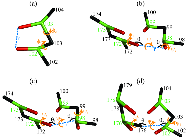
Figure S1: Geometrical parameters for (a) stacking in eq 1 and (c–d) hydrogen bonding in eq 5. Sites P, S and B are shown in black, green and red, respectively. Sample conformations are derived from 2K96.pdb. The numbers refer to specific nucleotides, and $r$, $\theta$, and $\phi$ or $\psi$ refer to distances (dist.), bond angles (ang.) and dihedral angles (dih.) between indicated sites. (a) Stacking: $r$ = dist. (B102, B103), $\phi_{1}$ = dih. (P102, S102, P103, S103), $\phi_{2}$ = dih. (P104, S103, P103, S102). (b) Hydrogen bonding between B and B: $r$ = dist. (B98, B172), $\theta_{1}$ = ang. (S172, B172, B98), $\theta_{2}$ = ang. (S98, B98, B172), $\psi$ = dih. (S98, B98, B172, S172), $\psi_{1}$ = dih. (B98, B172, S172, P173), $\psi_{2}$ = dih. (B172, B98, S98, P99). (c) Hydrogen bonding between B and S: $r$ = dist. (S98, B172), $\theta_{1}$ = ang. (S172, B172, S98), $\theta_{2}$ = ang. (P99, S98, B172), $\psi$ = dih. (P99, S98, B172, S172), $\psi_{1}$ = dih. (S98, B172, S172, P173), $\psi_{2}$ = dih. (B172, S98, P99, S99). (d) Hydrogen bonding between P and S: $r$ = dist. (S102, P176), $\theta_{1}$ = ang. (S176, P176, S102), $\theta_{2}$ = ang. (P103, S102, P176), $\psi$ = dih. (P103, S102, P176, S176), $\psi_{1}$ = dih. (S102, P176, S176, P178), $\psi_{2}$ = dih. (P176, S102, P103, S103).

We develop a realistic force field for nucleic acids using the TIS model ¹, in which each nucleotide is replaced by three spherical beads P, S and B, representing respectively a phosphate, a sugar and a base (Figure S1). The coarse-grained beads are at the center of mass of the chemical groups and have a radius $R_{i}$ of 2 Å for phosphates, 2.9 Å for sugars, 2.8 Å for adenines, 3 Å for guanines and 2.7 Å for cytosines and uracils. The values of $R_{i}$ are calculated using $V_{i}=4\pi R_{i}^{3}/3$, where $V_{i}$ is the van der Waals volume of the chemical group computed from the coordinates and radii of its individual atoms. We use the total molecular weight of each RNA group as the mass of the representative bead in our simulations. In the TIS representation of nucleic acids, bond lengths, $\rho$, and valence angles, $\alpha$, are constrained by harmonic potentials, $U(\rho)=k_{\rho}(\rho-\rho_{0})^{2}$ and $U(\alpha)=k_{\alpha}(\alpha-\alpha_{0})^{2}$, where the equilibrium values $\rho_{0}$ and $\alpha_{0}$ are obtained by coarse-graining an ideal A-form RNA helix². The values of $k_{\rho}$, in kcal mol^-1Å^-2, are: 64 for an S(5’)$-$P bond, 23 for an P$-$S(3’) bond and 10 for an S$-$B bond. The values of $k_{\alpha}$ are 5 kcal mol^-1rad^-2 if the valence angle involves a base, and 20 kcal mol^-1rad^-2 otherwise. We have chosen $k_{\rho}$ and $k_{\alpha}$ so that the time averages of $(\rho-\rho_{0})^{2}$ and $(\alpha-\alpha_{0})^{2}$ measured in simulations at $15\ ^{\circ}$C, match the corresponding quantities averaged over all bonds in the coarse-grained NMR structure of the hTR pseudoknot (PDB code 2K96).

Single strand stacking interactions, $U_{\mathrm{ST}}$, are applied to all pairs of consecutive nucleotides along the chain,

$$U_{\mathrm{ST}}=\frac{U_{\mathrm{ST}}^{0}}{1+1.4(r-r_{0})^{2}+4(\phi_{1}-\phi_{10})^{2}+4(\phi_{2}-\phi_{20})^{2}},$$ (1)

where $r$, $\phi_{1}$ and $\phi_{2}$ are defined in Figure S1a. The equilibrium values $r_{0}$, $\phi_{10}$ and $\phi_{20}$ are extracted from the coarse-grained structure of an ideal A-form RNA helix² and depend on the chemical identities of the two nucleotides. We obtain the constants $U_{\mathrm{ST}}^{0}$ for sixteen distinct nucleotide dimers from available experimental data on stacking of nucleic acid bases in single-stranded and double-stranded RNA ^{3, 4, 5}, as described next.

Additive contributions $\Delta G{b-c\choose a-d}$ of individual stacks to the total stability of an RNA double helix, where $a-d$ and $b-c$ are stacked Watson-Crick base pairs, are known experimentally ³. For reference, experimentally determined enthalpic $\Delta H{b-c\choose a-d}$ and entropic $\Delta S{b-c\choose a-d}$ contributions to $\Delta G{b-c\choose a-d}$ are reproduced in Table S1. We make the following approximations:

$$\Delta H{b-c\choose a-d} = \Delta H{b\choose a}+\Delta H{d\choose c}+0.5\Delta H(a-d)+0.5\Delta H(b-c),$$

$$\Delta S{b-c\choose a-d} = \Delta S{b\choose a}+\Delta S{d\choose c},$$ (2)

where $\Delta H{b\choose a}$ and $\Delta S{b\choose a}$ are the enthalpy and entropy changes resulting from stacking of $b$ over $a$ along $5^{\prime}\rightarrow 3^{\prime}$ in one strand, respectively, and $\Delta H(a-d)$ is the additional stability due to hydrogen bonding between $a$ and $d$ in two complementary strands. Inspection of $\Delta H{b-c\choose a-d}$ and $\Delta S{b-c\choose a-d}$ in Table S1 leads us to conclude that, except for ${\mathrm{C}\choose\mathrm{G}}$ and ${\mathrm{G}\choose\mathrm{C}}$, stacking parameters do not depend strongly on the order of nucleotides along $5^{\prime}\rightarrow 3^{\prime}$. Therefore, we assume, with the exception of ${\mathrm{C}\choose\mathrm{G}}$ and ${\mathrm{G}\choose\mathrm{C}}$, that $\Delta H{b\choose a}=\Delta H{a\choose b}$ and $\Delta S{b\choose a}=\Delta S{a\choose b}$, which is also valid within the range of experimental uncertainties specified in ref 2. This assumption allows us to average the experimental values for $\Delta H{\mathrm{U-A}\choose\mathrm{A-U}}$ and $\Delta H{\mathrm{A-U}\choose\mathrm{U-A}}$, $\Delta H{\mathrm{A-U}\choose\mathrm{C-G}}$ and $\Delta H{\mathrm{U-A}\choose\mathrm{G-C}}$, $\Delta H{\mathrm{U-A}\choose\mathrm{C-G}}$ and $\Delta H{\mathrm{A-U}\choose\mathrm{G-C}}$, and similarly for the corresponding entropies.

Based on the experimental data for stacking of nucleic acids in single-stranded RNA (see Table 8.1 in ref 3 and Table 1 in ref 4), we make additional assumptions that $\Delta H{\mathrm{C}\choose\mathrm{C}}=\Delta H{\mathrm{U}\choose\mathrm{C}}$, $\Delta H{\mathrm{A}\choose\mathrm{A}}=\Delta H{\mathrm{U}\choose\mathrm{A}}=\Delta H{\mathrm{C}\choose\mathrm{A}}$, and similarly for the entropies. This allows us to combine eq 2 for ${\mathrm{U-A}\choose\mathrm{A-U}}$ with the experimentally determined melting temperature $t_{m}{\mathrm{A}\choose\mathrm{A}}=26\ ^{\circ}$C⁴, which under our assumptions equals $t_{m}{\mathrm{U}\choose\mathrm{A}}$, and to solve for $\Delta H{\mathrm{U}\choose\mathrm{A}}$, $\Delta S{\mathrm{U}\choose\mathrm{A}}$ and $\Delta H(\mathrm{A}-\mathrm{U})$. Now putting $\Delta H{\mathrm{A}\choose\mathrm{A}}=\Delta H{\mathrm{U}\choose\mathrm{A}}$ and $\Delta S{\mathrm{A}\choose\mathrm{A}}=\Delta S{\mathrm{U}\choose\mathrm{A}}$ in eq 2 for ${\mathrm{A-U}\choose\mathrm{A-U}}$, we can compute $\Delta H{\mathrm{U}\choose\mathrm{U}}$ and $\Delta S{\mathrm{U}\choose\mathrm{U}}$. Finally, we assume

$$\Delta H{\mathrm{U}\choose\mathrm{C}}=k\Delta H{\mathrm{U}\choose\mathrm{A}}+(1-k)\Delta H{\mathrm{U}\choose\mathrm{U}},$$

$$\Delta S{\mathrm{U}\choose\mathrm{C}}=k\Delta S{\mathrm{U}\choose\mathrm{A}}+(1-k)\Delta S{\mathrm{U}\choose\mathrm{U}},$$ (3)

where $k=0.615$ yields $t_{m}{\mathrm{U}\choose\mathrm{C}}=13\ ^{\circ}$C, which matches the experimental result for $t_{m}{\mathrm{C}\choose\mathrm{C}}$⁴. The remaining stacking parameters follow directly from eq 2 without any additional approximations, if we use the computed hydrogen bond enthalpy $\Delta H(\mathrm{A}-\mathrm{U})=-1.47$ kcal/mol for an $\mathrm{A}-\mathrm{U}$ base pair and $3/2$ times this value for a $\mathrm{G}-\mathrm{C}$ pair. The resulting stacking parameters, which are used in the present simulations, are given in Table S2. The relative stabilities of stacks agree with the experimental data^{4, 6}, identifying $t_{m}{\mathrm{G}\choose\mathrm{G}}$ and $t_{m}{\mathrm{U}\choose\mathrm{U}}$ as the highest and lowest melting temperatures among all stacks.

We simulated stacking of nucleotide dimers, similar to that shown in Figure S1a, using the stacking potential $U_{\mathrm{ST}}$ in eq 1 and $U_{\mathrm{ST}}^{0}=-h+k_{\mathrm{B}}(T-T_{m})s$, where $k_{\mathrm{B}}$ is the Boltzmann constant, $T$ (K) is the absolute temperature, $T_{m}$ (K) is the melting temperature of each stack (from Table S2) and $h$ and $s$ are adjustable parameters. In our simulations, we computed the stability $\Delta G(T)$ of stacks at temperature $T$ as

$$\Delta G(T)=-k_{\mathrm{B}}T\log{N_{1}}+k_{\mathrm{B}}T\log{N_{2}}+\Delta G_{0},$$ (4)

where $N_{1}$ is the number of all stacked configurations for which $U_{\mathrm{ST}}<-k_{\mathrm{B}}T$ and $N_{2}$ is the number of all unstacked configurations. We adjusted $h$ and $s$ individually for all stacks so that the simulation results for $\Delta H$ and $\Delta S$, given by $\Delta G(T)=\Delta H-T\Delta S$, matched the corresponding values in Table S2. The stability correction $\Delta G_{0}$ in eq 4 is assumed to be constant for all stacks and accounts for potential discrepancies between $\Delta G(T)$ measured in experiments and its definition used in our simulations.

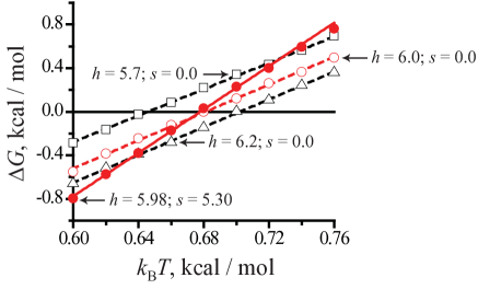
Figure S2: Stability $\Delta G(T)$ of stack ${\mathrm{G}\choose\mathrm{A}}$, computed from eq 4 with $\Delta G_{0}=0$, in simulations with the stacking potential given by eq 1 and $U_{\mathrm{ST}}^{0}=-h+k_{\mathrm{B}}(T-T_{m})s$. $T_{m}$ indicates the melting temperature for ${\mathrm{G}\choose\mathrm{A}}$ from Table S2, $k_{\mathrm{B}}T_{m}=0.68$ kcal/mol. Open and closed symbols show simulation results for various $h$ and $s$. Red solid line indicates the target stability $\Delta G(T)=\Delta H-T\Delta S$ for ${\mathrm{G}\choose\mathrm{A}}$, where $\Delta H$ and $\Delta S$ are given in Table S2. Same stability line is obtained in simulation with $h=5.98$ kcal/mol and $s=5.30$ (closed symbols).

As an example, in Figure S2 we plot $\Delta G(T)$ obtained in simulations of the ${\mathrm{G}\choose\mathrm{A}}$ stack with various values of $h$ and $s=0$. The simulation results in Figure S2 are shown for $\Delta G_{0}=0$. The observed melting temperature $T^{*}$, defined as $\Delta G(T^{*})=0$, increases with $h$ and equals the target melting temperature $T_{m}{\mathrm{G}\choose\mathrm{A}}$ in Table S2 when $h=5.98$ kcal/mol. For $s=0$ the entropy loss $\Delta S$ associated with stack formation, given by the slope of $\Delta G(T)$ over $T$, is smaller than the value of $\Delta S{\mathrm{G}\choose\mathrm{A}}$ specified in Table S2. To correct this, we use $U_{\mathrm{ST}}^{0}=-5.98+k_{\mathrm{B}}(T-T_{m})s$, which does not result in changes in the melting temperature but allows us to adjust the slope of $\Delta G(T)$ by adjusting the value of $s$. We find that $s=5.30$ yields $\Delta S{\mathrm{G}\choose\mathrm{A}}$ in Table S2.

We carried out the same fitting procedure for all nucleotide dimers. The resulting parameters $U_{\mathrm{ST}}^{0}$ for $\Delta G_{0}=0$ and $\Delta G_{0}=0.5$ kcal/mol are summarized in Table S3. In our simulations, we use the value $\Delta G_{0}=0.5$ kcal/mol which yields the best agreement with experiments (see discussion in the last section below). Note that, although some stacks have equivalent thermodynamic parameters in Table S2, they may require somewhat different $U_{\mathrm{ST}}^{0}$ due to their geometrical differences.

Coarse-grained hydrogen bond interactions $U_{\mathrm{HB}}$ are assigned based on the hydrogen bonds present in the original NMR structure. In this work, we carried out independent simulations of the pseudoknot and hairpin conformations of the hTR pseudoknot domain (PDB codes 2K96 and 1NA2, respectively). In both cases, we generated an optimal network of hydrogen bonds by submitting the NMR structure to the WHAT IF server at http://swift.cmbi.ru.nl. Each of the generated bonds is modeled by a coarse-grained interaction potential,

$$U_{\mathrm{HB}}=2.286\times\left[1+5(r-r_{0})^{2}+1.5(\theta_{1}-\theta_{10})^{2}+1.5(\theta_{2}-\theta_{20})^{2}\right.$$

$$\left.+0.15(\psi-\psi_{0})^{2}+0.15(\psi_{1}-\psi_{10})^{2}+0.15(\psi_{2}-\psi_{20})^{2}\right]^{-1},$$ (5)

where $r$, $\theta_{1}$, $\theta_{2}$, $\psi$, $\psi_{1}$ and $\psi_{2}$ for various coarse-grained sites are defined in Figure S1. In the case of Watson-Crick base pairs, the equilibrium values $r_{0}$, $\theta_{10}$, $\theta_{20}$, $\psi_{0}$, $\psi_{10}$ and $\psi_{20}$ are adopted from the coarse-grained structure of an ideal A-form RNA helix². For all other bonds, the equilibrium parameters are obtained by coarse-graining the PDB structure itself. Equation 5 specifies $U_{\mathrm{HB}}$ for a single hydrogen bond and it must be multiplied by a factor of 2 or 3 if the same coarse-grained sites are connected by more than one hydrogen bond. The complex geometry of $U_{\mathrm{HB}}$ is the minimum necessary to maintain stable double (and triple) helices in our coarse-grained model.

2 Comparison of two alternative sets of interaction parameters

In our simulations, stacking parameters $U_{\mathrm{ST}}^{0}$ are determined based on the definition of $\Delta G(T)$ given in eq 4. The corrective constant $\Delta G_{0}=0.5$ kcal/mol in eq 4 is introduced to improve quantitative agreement between simulation and experimental melting data of the hTR pseudoknot domain. If $\Delta G_{0}$ were omitted from eq 4, this would result in stronger stacking interactions (see Table S3). In order to preserve overall melting temperatures, this increase in the magnitude of $U_{\mathrm{ST}}^{0}$ must be compensated for by a decrease in the strength of hydrogen bonds. For $\Delta G_{0}=0$, the best agreement with experiments is achieved when the prefactor in eq 5 is reduced to 2.065.

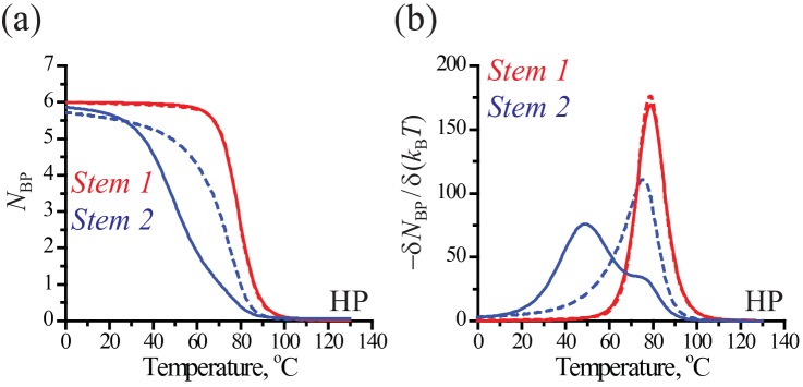
Figure S3: (a) Number of intact base pairs $N_{\mathrm{BP}}$ vs. temperature in two elements of secondary structure in HP. (b) The melting profiles show the rate of change of the number of intact base pairs with temperature. The data are obtained for different values of $\Delta G_{0}$ in eq 4: 0.5 kcal/mol (solid) and 0 (dashed).

In Figure S3 we compare melting data for the hairpin (HP) conformation of the hTR pseudoknot domain for the two parameter sets, with and without the corrective constant $\Delta G_{0}$. The melting profile of the Watson-Crick part of the double helix, stem 1 in HP, is hardly affected by the choice of $U_{\mathrm{ST}}^{0}$. However, we observe a large discrepancy for the uridine-rich stem 2, whose melting temperature increases from 50 ^∘C to 75 ^∘C if $\Delta G_{0}$ is set to 0 in eq 4. In the latter case, the total melting profile of HP shows only one peak at 78 ^∘C, which does not compare well with two experimental peaks at 50 ^∘C and 79 ^∘C⁷. We conclude that the corrective constant in eq 4 is crucial for obtaining quantitative agreement with the experimental data for HP.

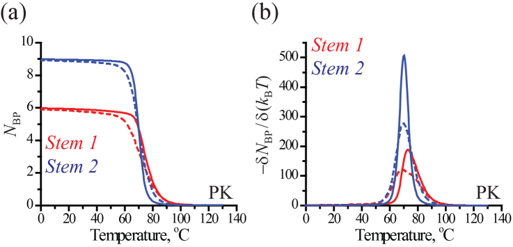
Figure S4: Same as in Figure S3, but for the PK conformation.

Melting of secondary structure in the pseudoknot (PK) conformation of the hTR pseudoknot domain is compared in Figure S4 for $\Delta G_{0}=0.5$ kcal/mol and $\Delta G_{0}=0$. In experiments⁸, the temperature range for melting of stems 1 and 2 in PK is 65–95 ^∘C and 60–80 ^∘C, respectively. As shown in Figure S4, these experimental data are reproduced well in simulations with $\Delta G_{0}=0.5$ kcal/mol (weak stacks in Table S3 and $U_{\mathrm{HB}}^{0}=2.286$). At the same time, for $\Delta G_{0}=0$ (strong stacks in Table S3 and $U_{\mathrm{HB}}^{0}=2.065$), melting of both stems occurs in the temperature range 50–95 ^∘C. For both parameter sets, the overall melting profile of PK has a sharp peak at 70 ^∘C, in agreement with experiments⁸.

The distance between two peaks in the melting profile of HP increases with $\Delta G_{0}$ and exceeds the experimental distance when $\Delta G_{0}>0.5$ kcal/mol (data not shown). We therefore conclude that, for both conformations of the hTR pseudoknot domain, the parameter model based on $\Delta G_{0}=0.5$ kcal/mol yields the optimal agreement with experimental thermodynamic data.

3 Crowder-RNA interactions

Crowder-RNA interactions are modeled by a generalized Lennard-Jones potential,

$$U_{\mathrm{LJ}}(r) = \varepsilon\frac{2R_{i}}{D_{0}}\left[\left(\frac{D_{0}}{r+D_{0}-D}\right)^{12}-2\left(\frac{D_{0}}{r+D_{0}-D}\right)^{6}+1\right],\ r\leq D,$$

$$U_{\mathrm{LJ}}(r) = 0,\ r>D,$$ (6)

where $r$ is the distance between the particles’ centers of mass, $D_{0}=3.2$ Å is the effective penetration depth, $R_{i}$ is the radius of an RNA coarse-grained bead (values specified above), $r_{\mathrm{C}}$ is the radius of a crowder, and $D=R_{i}+r_{\mathrm{C}}$. The ratio $2R_{i}/D_{0}$ in eq 6 is used to scale the interaction strength $\varepsilon=1$ kcal/mol in proportion to the surface contact area.

We use the same formula to model RNA-RNA excluded volume interactions, but take $R_{i}=1.6$ Å for all RNA beads. In this case, eq 6 becomes a standard (purely repulsive) Lennard-Jones potential,

$$U_{\mathrm{LJ}}(r) = \varepsilon\left[\left(\frac{D_{0}}{r}\right)^{12}-2\left(\frac{D_{0}}{r}\right)^{6}+1\right],\ r\leq D_{0},$$

$$U_{\mathrm{LJ}}(r) = 0,\ r>D_{0}.$$ (7)

With adjustment of $R_{i}$ steric clashes between two stacked bases are avoided.

4 Simulation details

The RNA and crowder dynamics are simulated by solving the Langevin equation, which for particle $i$ is $m_{i}\ddot{\mathbf{r}}_{i}=-\gamma_{i}\dot{\mathbf{r}}_{i}+\mathbf{F}_{i}+\mathbf{R}_{i}$, where $m_{i}$ is the particle mass, $\gamma_{i}$ is the drag coefficient, $\mathbf{F}_{i}$ is the conservative force, and $\mathbf{R}_{i}$ is the Gaussian random force, $\left<\mathbf{R}_{i}(t)\mathbf{R}_{j}(t^{\prime})\right>=6k_{\mathrm{B}}T\gamma_{i}\delta_{ij}\delta(t-t^{\prime})$. The drag coefficient is given by the Stokes formula, $\gamma_{i}=6\pi\eta R_{i}$, where $\eta$ is the viscosity of the medium and $R_{i}$ is the particle radius. To enhance conformational sampling, we take $\eta=10^{-5}$Pa$\cdot$s, which equals approximately 1% of the viscosity of water. The masses and radii of RNA coarse-grained beads are specified above. The masses of crowders scale with their volume, assuming density equal to that of a typical folded protein such as ubiquitin, which has the molecular weight $M_{\mathrm{r}}=8564$ Da and radius $r_{\mathrm{C}}=1.2$ nm. The Langevin equation is integrated using the leap-frog algorithm with time step $\Delta t=2.5$ fs. The length of a simulation run at each temperature is 2.5 $\mu$s.

The number of crowders of a given type is computed from its specified volume fraction and the volume of the simulation box. In simulations with large crowders ($r_{\mathrm{C}}=10.4$ nm, 5.2 nm and 2.6 nm) we use 60 nm as the side of the cubic simulation box. For example, the E. coli mixture contains the volume fractions $\phi_{1}=0.11$, $\phi_{2}=0.11$ and $\phi_{3}=0.08$ of crowders with $r_{\mathrm{C}}=10.4$ nm, 5.2 nm and 2.6 nm, respectively. For a simulation box with side 60 nm, this yields 5 crowders with $r_{\mathrm{C}}=10.4$ nm, 40 with $r_{\mathrm{C}}=5.2$ nm and 234 with $r_{\mathrm{C}}=2.6$ nm (279 crowders in total). In simulations with small crowders ($r_{\mathrm{C}}=1.2$ nm and 0.6 nm) the number of crowders in the cubic box with side 60 nm becomes very large. To minimize simulation time of these systems, the size and shape of the simulation box is adjusted periodically to accommodate RNA in its current conformation. To do so, we first align the walls of the box with the RNA axes of inertia. The new position of the RNA center of mass and new side lengths $L_{x}$, $L_{y}$, $L_{z}$ are computed so that there is at least a 6 nm distance between each RNA bead and all six walls. When, as a result of diffusion, the distance between an RNA bead and a wall becomes less than 2.4 nm, the box is adjusted again. The size and shape of the simulation box are therefore directly coupled to the RNA configuration. For instance, in simulations at 0 ^∘C, the RNA remains folded and $L_{x}$, $L_{y}$, $L_{z}$ fluctuate around 18 nm, 15 nm and 14 nm, respectively (assuming $L_{x}>L_{y}>L_{z}$). In simulations at 120 ^∘C, the RNA is unfolded and the average lengths are $L_{x}=20$ nm, $L_{y}=16.5$ nm and $L_{z}=15$ nm. In simulations at intermediate temperatures, when the RNA folds and unfolds, the size of the box undergoes large fluctutions between the high-temperature and low-temperature values. The frequency with which the simulation box is adjusted also depends on the temperature through RNA diffusion. The box is adjusted approximately every 1200000 steps at 0 ^∘C and every 700000 steps at 120 ^∘C. When the box is adjusted, the number of crowders changes with the new box volume in order to keep the volume fractions $\phi$ constant.

Table S1: Thermodynamic parameters of double-stranded stacks from ref 2. In the first column, the $5^{\prime}$ to $3^{\prime}$ direction is shown by an arrow.

$\uparrow{b-c\atop a-d}\downarrow$	$\Delta H$, kcal mol-1	$\Delta S$, cal mol-1K-1
$\mathrm{A-U}\atop\mathrm{A-U}$	$-6.82$	$-19.0$
$\mathrm{U-A}\atop\mathrm{A-U}$	$-9.38$	$-26.7$
$\mathrm{A-U}\atop\mathrm{U-A}$	$-7.69$	$-20.5$
$\mathrm{U-A}\atop\mathrm{C-G}$	$-10.48$	$-27.1$
$\mathrm{A-U}\atop\mathrm{C-G}$	$-10.44$	$-26.9$
$\mathrm{U-A}\atop\mathrm{G-C}$	$-11.40$	$-29.5$
$\mathrm{A-U}\atop\mathrm{G-C}$	$-12.44$	$-32.5$
$\mathrm{G-C}\atop\mathrm{C-G}$	$-10.64$	$-26.7$
$\mathrm{G-C}\atop\mathrm{G-C}$	$-13.39$	$-32.7$
$\mathrm{C-G}\atop\mathrm{G-C}$	$-14.88$	$-36.9$

Table S2: Thermodynamic parameters of single-stranded stacks, derived in this work. The matching enthalpies of hydrogen bond formation in Watson-Crick base pairs are given in last two rows. The melting temperatures of stacks are indicated in ^∘C, $t_{m}(^{\circ}\mathrm{C})=T_{m}(\mathrm{K})-273.15$. In the first column, the $5^{\prime}$ to $3^{\prime}$ direction is shown by an arrow.

$\uparrow{b\atop a}$	$\Delta H$, kcal mol-1	$\Delta S$, cal mol-1K-1	$t_{m}$,∘C
$\mathrm{U}\atop\mathrm{U}$	$-1.81$	$-7.2$	$-21$
$\mathrm{C}\atop\mathrm{C}$	$-2.87$	$-10.0$	13
$\mathrm{C}\atop\mathrm{U}$; $\mathrm{U}\atop\mathrm{C}$	$-2.87$	$-10.0$	13
$\mathrm{A}\atop\mathrm{A}$	$-3.53$	$-11.8$	26
$\mathrm{A}\atop\mathrm{U}$; $\mathrm{U}\atop\mathrm{A}$	$-3.53$	$-11.8$	26
$\mathrm{A}\atop\mathrm{C}$; $\mathrm{C}\atop\mathrm{A}$	$-3.53$	$-11.8$	26
$\mathrm{G}\atop\mathrm{C}$	$-4.21$	$-13.3$	42
$\mathrm{G}\atop\mathrm{U}$; $\mathrm{U}\atop\mathrm{G}$	$-5.55$	$-16.4$	65
$\mathrm{C}\atop\mathrm{G}$	$-6.33$	$-18.4$	70
$\mathrm{G}\atop\mathrm{A}$; $\mathrm{A}\atop\mathrm{G}$	$-6.75$	$-19.8$	68
$\mathrm{G}\atop\mathrm{G}$	$-8.31$	$-22.7$	93
$\Delta H(\mathrm{A}-\mathrm{U})=-1.47$ kcal/mol
$\Delta H(\mathrm{G}-\mathrm{C})=-2.21$ kcal/mol

Table S3: Temperature-dependent stacking parameters $U_{\mathrm{ST}}^{0}$ used in eq 1. The two sets of $h$ correspond to two different values of the additive constant $\Delta G_{0}$ in eq 4: 0.5 kcal/mol and 0 (numbers in brackets). The melting temperatures $T_{m}$ of individual stacks are given in Table S2. The values of $s$ conform to $k_{\mathrm{B}}(T-T_{m})$ evaluated in kcal mol^-1. In the first column, the $5^{\prime}$ to $3^{\prime}$ direction is shown by an arrow.

	$U_{\mathrm{ST}}^{0}=-h+k_{\mathrm{B}}(T-T_{m})s$
$\uparrow{b\atop a}$	$h$, kcal mol-1	$s$
$\mathrm{U}\atop\mathrm{U}$	3.52 (4.27)	$-3.56$
$\mathrm{C}\atop\mathrm{C}$	4.16 (4.87)	$-1.57$
$\mathrm{C}\atop\mathrm{U}$; $\mathrm{U}\atop\mathrm{C}$	4.14 (4.88); 4.14 (4.87)	$-1.57$; $-1.57$
$\mathrm{A}\atop\mathrm{A}$	4.49 (5.19)	$-0.32$
$\mathrm{A}\atop\mathrm{U}$; $\mathrm{U}\atop\mathrm{A}$	4.43 (5.16); 4.45 (5.15)	$-0.32$; $-0.32$
$\mathrm{A}\atop\mathrm{C}$; $\mathrm{C}\atop\mathrm{A}$	4.43 (5.16); 4.45 (5.15)	$-0.32$; $-0.32$
$\mathrm{G}\atop\mathrm{C}$	4.75 (5.48)	0.77
$\mathrm{G}\atop\mathrm{U}$; $\mathrm{U}\atop\mathrm{G}$	5.17 (5.89); 5.12 (5.84)	2.92; 2.92
$\mathrm{C}\atop\mathrm{G}$	5.22 (5.93)	4.37
$\mathrm{G}\atop\mathrm{A}$; $\mathrm{A}\atop\mathrm{G}$	5.26 (5.98); 5.22 (5.95)	5.30; 5.30
$\mathrm{G}\atop\mathrm{G}$	5.70 (6.42)	7.35

Figure S5: Temperature dependence of the stabilities of the hairpin and pseudoknot in the absence of crowders (solid) and in a monodisperse suspension of crowders with $\phi=0.3$ and $r_{\mathrm{C}}=1.2$ nm (dashed). (a) $\Delta$U177 sequence. (b) $\Delta$U177 sequence with DKC mutations.

Figure S6: (a) Changes in stability (kcal/mol) of HP and PK at 37 ^∘C due to crowders, as a function of the crowder radius $r_{\mathrm{C}}$. (b) Probability distributions $p(R_{\mathrm{G}})$ of the radius of gyration of the unfolded HP and PK structures at 37 ^∘C in the absence of crowders ($\phi=0$). $R_{\mathrm{G}}$ of HP is defined as the radius of gyration of strand G93–C121, which is the only fragment that is structured in HP (same definition is used in the paper). $R_{\mathrm{G}}$ of PK is computed for the entire length of RNA. The unfolded state cannot be sampled directly in simulations at 37 ^∘C and the shown $p(R_{\mathrm{G}})$ are obtained by statistical reweighting of the high-temperature data. For PK, $p(R_{\mathrm{G}})$ is noticeably asymmetric, showing an extended tail on the side of large $R_{\mathrm{G}}$. This is in part due to residual stacking in the unfolded state, whose effects become more pronounced for longer strands. A larger mean of $p(R_{\mathrm{G}})$ and its asymmetry explain why the PK structure is more strongly influenced by crowders than HP. (c)–(d) $p(R_{\mathrm{G}})$ in crowder suspensions with $\phi=0.3$ and different $r_{\mathrm{C}}$. Symbols match those in panel (a) and black solid curves show $p(R_{\mathrm{G}})$ at $\phi=0$. In all four panels, dashed curves are drawn through data to facilitate comparison.

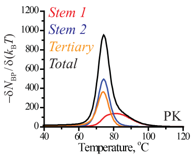
Figure S7: Same as in Figure 2a of the main text, but in a monodisperse suspension of crowders with $\phi=0.3$ and $r_{\mathrm{C}}=1.2$ nm.

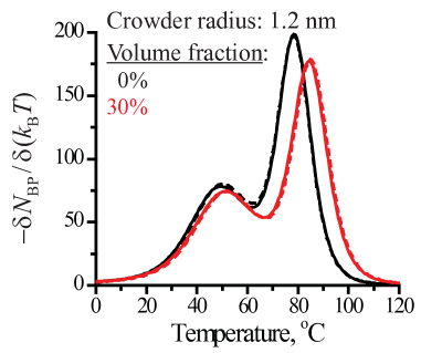
Figure S8: Melting profiles of the hairpin in the absence of crowders (black) and in a monodisperse suspension of crowders with $\phi=0.3$ and $r_{\mathrm{C}}=1.2$ nm. Dashed and solid curves are for the $\Delta$U177 sequence with and without additional DKC mutations.

References

- 1 Hyeon, C.; Thirumalai, D. Proc. Natl. Acad. Sci. U.S.A 2005, 102, 6789–6794.
- 2 A sample A-form RNA structure can be found at http://www.biochem.umd.edu/ biochem/kahn/teach_res/dna_tutorial/.
- 3 Xia, T.; SantaLucia, J., Jr.; Burkand, M. E.; Kierzek, R.; Schroeder, S. J.; Jiao, X.; Cox, C.; Turner, D. H. Biochemistry 1998, 37, 14719–14735.
- 4 Bloomfield, V. A.; Crothers, D. M.; Tinoco, I., Jr. Nucleic Acids: Structures, Properties, and Functions, 1st ed.; University Science Books, 2000.
- 5 Dima, R. I.; Hyeon, C.; Thirumalai, D. J. Mol. Biol. 2005, 347, 53–69.
- 6 Florián, J.; Šponer, J.; Warshel, A. J. Phys. Chem. B 1999, 103, 884–892.
- 7 Comolli, L. R.; Smirnov, I.; Xu, L.; Blackburn, E. H.; James, T. L. Proc. Natl. Acad. Sci. U.S.A 2002, 99, 16998-17003.
- 8 Theimer, C. A.; Blois, C. A.; Feigon, J. Mol. Cell 2005, 17, 671–682.