Modeling electrostatic patch effects in Casimir force measurements

Abstract

Electrostatic patch potentials give rise to forces between neutral conductors at distances in the micrometer range and must be accounted for in the analysis of Casimir force experiments. In this paper we develop a quasi-local model for describing random potentials on metallic surfaces. In contrast to some previously published results, we find that patches may provide a significant contribution to the measured signal, and thus may be a more important systematic effect than was previously anticipated. Additionally, patches may render the experimental data at distances below 1 micrometer compatible with theoretical predictions based on the Drude model.

I Introduction

The Casimir effect Casimir48 ; Lamoreaux05 ; Bordag09 ; Dalvit11 is a remarkable consequence of vacuum field fluctuations which, in its simplest manifestation, leads to the attraction of two neutral ideal conducting plates. At very short distances quantum fluctuation forces dominate the interaction between neutral objects making them an essential consideration for micro-electro mechanical devices (MEMS) and atom traps, among others. The comparison between experimental measurements and theory for Casimir forces between metallic plates has been a matter of debate in recent years. This debate is of particular importance if this comparison is used to derive constraints on hypothetical new short-range interactions appearing in addition to the gravity force in unification models Fischbach98 ; Adelberger03 ; Onofrio06 ; Antoniadis11 .

Two recent experiments are at the heart of this debate. Casimir force measurements by the IUPUI group Decca05 ; Decca07 , performed at distances smaller than 750 nm, were interpreted by the authors as excluding the dissipative Drude model and agreeing with the lossless plasma model. This has led to a discrepancy between experiments and physically motivated theoretical models, such as the Drude model, for real conductors which exhibit dissipation. In distinction, a recent experiment by the Yale Sushkov11 was able to measure Casimir forces at distances up to 7 $\mu$m and was interpreted by the authors as being in agreement with the Drude prediction, including quantum as well as thermal fluctuations, once an electrostatic patch contribution has been taken into account.

It is known that patch effects are a source of concern for Casimir experiments Speake03 ; Chumak04 ; Kim10 ; deMan10 ; Kim10b , as well as for other precision measurements Fairbank67 ; Camp91 ; Turchette00 ; Deslauriers06 ; Robertson06 ; Epstein07 ; Pollack08 ; Adelberger09 ; Everitt11 ; Reasenberg11 . For the Yale experiment the patches were assumed to be much larger than the gap $D$ between the spherical and planar plates used in the measurement. Under these conditions the patch force is found to be proportional to $RV^{2}_{\mathrm{rms}}/D$ in the proximity force approximation (see below), where $R$ is the radius of curvature of the spherical plate and $V_{\mathrm{rms}}$ is the root-mean-square (rms) voltage of electrostatic patch potentials Sushkov11 . For the IUPUI experiment, a patch analysis was performed with different assumptions leading to the conclusion that the patch effect had a negligible influence Decca05 . Unfortunately, it was not possible in any of these experiments to measure the patches independently. It follows that the conclusions of the theory-experiment comparisons heavily rely on the patch models used in the data analysis.

In this paper, we revisit electrostatic patch effects and analyze their possible influence in Casimir force measurements. Our approach is based on the method pioneered by Speake and Trenkel Speake03 with the electrostatic patches described in terms of a power spectral density. However, we will develop a model for the power spectral density differing from the one proposed in Speake03 and used in Decca05 ; Decca07 .

Our model is based on the observation that bare metallic surfaces are composed of crystallites, each of which constitutes a single patch, where the local surface voltage is determined by the local work function Gaillard06 . By assuming that through the surface preparation process the crystallographic orientation, and hence the corresponding work function, of each crystallite is determined independently and randomly we can infer that voltage correlations are restricted to points lying on the same patch: We refer to this as quasi-local correlation. Our model with quasi-local correlations can be compared to the case of quenched charge disorder in dielectrics Naji10 ; Sarabadani10 , and also shows close similarities with models proposed recently to describe patch correlation functions for atomic or ionic traps Dubessy09 ; Carter11 .

We will show that the voltage correlation function from our quasi-local model strongly differs from that initially proposed in Speake03 and used in Decca05 ; Decca07 . As a result, in contrast to the claims of Decca05 ; Decca07 , patches may have a significant contribution to the IUPUI measurements. In addition we will qualitatively address the issue of surface contamination which is expected to lead to larger correlation lengths and reduced voltage fluctuations Rossi92 . Given that the degree of contamination is unknown we perform a fit of the patch model we propose to the difference between measurements and the Casimir theoretical prediction based on the Drude model and find that it qualitatively explains the residual signal. For the Yale experiment, our results will essentially reproduce those obtained in Sushkov11 .

II Electrostatic patch effect

In the present section, we recall a few general results of interest, assuming that the validity conditions of the proximity force approximation (PFA) are satisfied, that is, the radius of the sphere used in the experiment is much greater than the sphere-plane distance. In this case, the expression for the force gradient $G_{sp}$ (derivative with distance of the force $F_{sp}$) in the sphere-plane geometry is written as follows in terms of the pressure $P_{pp}$ (the force per unit area) calculated between two planes

$$G_{sp}(D)\equiv\frac{\partial F_{sp}(D)}{\partial D}=2\pi RP_{pp}(D).$$ (1)

This expression is used throughout the paper for both Casimir and patch effects.

The basic description of the patch effect after Speake03 is a statistical ensemble of patch potentials $V_{i}({\bf r})$ on the surfaces of two planar plates labeled $i=1,2$. The potentials are assumed to have zero mean $\langle V_{i}({\bf r})\rangle=0$, and to be described by the two-point potential correlation functions

$$C_{ij}({\bf r})=\langle V_{i}({\bf r})V_{j}({\bf 0})\rangle=\int\frac{d^{2}{\bf k}}{4\pi^{2}}e^{i{\bf k}\cdot{\bf r}}C_{ij}[\bf k].$$ (2)

In the plane-plane geometry, points on the planes are denoted in cartesian coordinates as ${\bf r}=(x,y)$ and the point ${\bf 0}$ is an arbitrary origin. The correlation functions $C_{ij}({\bf r})$ and therefore the power spectra $C_{ij}[\bf k]$ are also assumed to be isotropic. The relations between these two functions can be written

$$C_{ij}(r)=\frac{1}{2\pi}\int_{0}^{\infty}dk\ k\ J_{0}(kr)\ C_{ij}[k],$$

$$C_{ij}[k]=2\pi\int_{0}^{\infty}dr\ r\ J_{0}(kr)\ C_{ij}(r),$$ (3)

where we have simply denoted $r\equiv|{\bf r}|$ and $k\equiv|{\bf k}|$ and where $J_{n}(x)$ is the n-th order Bessel function Gradshteyn . The patch power spectrum $C_{ij}[k]$ corresponds to the notation $\tilde{C}_{ij}(k)$ in Speake03 . As usual, the variances and covariances are given by the integrals

$$C_{ij}(0)=\langle V_{i}V_{j}\rangle=\frac{1}{2\pi}\int_{0}^{\infty}dk\ k\ C_{ij}[k].$$ (4)

The pressure due to electrostatic patches in the plane-plane geometry can be computed exactly Speake03 as

$$P_{pp}^{\mathrm{patch}}(D) = \frac{\varepsilon_{o}}{4\pi}\int_{0}^{\infty}\frac{dk\ k^{3}}{\sinh^{2}(kD)}$$

$$\times\left\{C_{11}[k]+C_{22}[k]-2C_{12}[k]\cosh(kD)\right\}.$$

It is worth emphasizing at this point that the integral is reduced to a very simple expression when patch sizes, with a typical value denoted $\ell_{\mathrm{patch}}$, are larger than the distance $D$. In this case, all wavevectors $k$ contributing to the integral (II) satisfy $kD\ll 1$, so that the pressure scales universally as $1/D^{2}$, irrespective of the particular details of the power spectrum (Eq. (4) is used)

$$P_{pp}^{\mathrm{patch}}(D) = \frac{\varepsilon_{o}}{2D^{2}}\int_{0}^{\infty}\frac{dk\ k}{2\pi}\left\{C_{11}[k]+C_{22}[k]-2C_{12}[k]\right\}$$ (6)

$$= \frac{\varepsilon_{o}}{2D^{2}}\left\langle\left(V_{i}-V_{j}\right)^{2}\right\rangle\quad,\quad D\ll\ell_{\mathrm{patch}}.$$

The above result is expected from the analogy with a parallel plate capacitor with prescribed voltages. In contrast, when the relevant wavevectors no longer satisfy the above inequality, different models for the patch power spectrum result in different predictions for the patch contribution to the pressure.

It is also worth mentioning here some conditions for the expression (II) of the electrostatic patch pressure between two plates to be valid. A fundamental assumption in this analysis is that the ergodic hypothesis is satisfied, which means that the distribution of patches within the interaction area is a fair approximation of the ensemble-averaged distribution function defined by the power spectrum $C_{ij}[k]$. When applied to two plane plates of finite area $A$, we expect this assumption to be well satisfied if the effective interaction area contains a large number of patch correlation areas $A\gg\ell_{\mathrm{patch}}^{2}$. For the sphere-plane geometry, the effective area of interaction is of the order of $\pi DR$, leading to the validity requirement

$$\pi DR\gg\ell_{\mathrm{patch}}^{2}.$$ (7)

In the following two subsections we recall a model used in Speake03 and Decca05 ; Decca07 , and introduce another model with quasi-local correlations which we think to be a better description of sputtered surfaces.

II.1 The sharp-cutoff model

We now discuss the model of patch correlations which was proposed as an example in Speake03 and then used in Decca05 ; Decca07 to assess the contribution of electrostatic patches to the Casimir force measurements.

It is a simple description based upon two assumptions: a) the power spectrum of patches is an annulus in $k$-space possessing no other dependence than a sharp cutoff at small ($k_{\mathrm{min}}$) and large ($k_{\mathrm{max}}$) wavevectors (hence the name sharp-cutoff model); b) there are no cross correlations between the two plates ($C_{12}=0$). This model gives the power spectrum for a single plate as

$$C_{ii}[k]=\frac{4\pi V_{\mathrm{rms}}^{2}}{k_{\mathrm{max}}^{2}-k_{\mathrm{min}}^{2}}\theta(k_{\mathrm{max}}-k)\theta(k-k_{\mathrm{min}}),$$ (8)

where $V_{\mathrm{rms}}^{2}$ is the variance of the potential on one plate and $\theta$ is the Heaviside step function.

In order to determine the parameters of this model, the authors of Decca05 used the further assumptions : c) based on AFM images of the surfaces, the minimum and maximum grain sizes of the samples were determined to be $\ell_{\mathrm{patch}}^{\mathrm{min}}=25$ nm and $\ell_{\mathrm{patch}}^{\mathrm{max}}=300$ nm  ; d) the patch sizes were assumed to be the same as the grain sizes and the cutoffs in $k$-space were derived from the inverse maximum and minimum grain sizes $k_{\mathrm{min}}=2\pi/\ell_{\mathrm{patch}}^{\mathrm{max}}=20.9\mu\mathrm{m}^{-1}$ and $k_{\mathrm{max}}=2\pi/\ell_{\mathrm{patch}}^{\mathrm{min}}=251\mu\mathrm{m}^{-1}$  ; e) the rms voltage was obtained by computing the variance of the work functions over the different crystallographic planes of gold, which led to $V_{\mathrm{rms}}\approx 80.8$ mV. Using the five assumptions a) to e), it was concluded in Decca05 that the patch pressure had a negligible influence on the estimation of the Casimir force. A reasonable agreement was then obtained between the experimental data and the prediction for the Casimir pressure using the lossless plasma model (more discussions below).

Now we will argue that model (8) is not a good description for the patch power spectrum for the surfaces used in the experiments, and later on, we will also question the relation between patch and grain sizes. In order to make the former point clear, let us write the correlation function $C_{ii}(r)$ of patches in real space which can be obtained through an inverse Fourier transform (II) from the spectrum (8)

$$C_{ii}(r)=2V_{\mathrm{rms}}^{2}\frac{k_{\mathrm{max}}J_{1}(k_{\mathrm{max}}r)-k_{\mathrm{min}}J_{1}(k_{\mathrm{min}}r)}{\left(k_{\mathrm{max}}^{2}-k_{\mathrm{min}}^{2}\right)r}.$$ (9)

As one moves away from coincidence the correlation function $C_{ii}(r)$ oscillates between positive and negative values with a period of the order of the smallest patch size, and is contained within an envelope decaying as $r^{-3/2}$ (see Fig.1). These oscillations imply that the patch potential shows correlations as well as anti-correlations in space. Such behavior could be expected for surfaces exhibiting some kind of antiferroelectric ordering (where the configurational energy is minimized when adjacent surface dipoles are antiparallel), but will unlikely describe the random potentials on sputtered surfaces.

Figure 1: Comparison of the sharp-cutoff and quasi-local patch models described in subsections II-A (dashed lines) and II-B (solid lines), respectively. Plot (a) shows the voltage correlation functions in real space while plot (b) shows the associated spectrum in Fourier space. All plots correspond to the correlation function $C\equiv C_{ii}$ divided by $V_{\mathrm{rms}}^{2}$. On the lower plot, the sharp-cutoff spectrum discussed in II-A is multiplied by a factor of $100$ in order for it to appear at the scales shown. The parameters used for both models, discussed in subsections II-A and II-B, are taken from Decca05 , but however, do not correspond to the same average patch size.

As already stated, the strict relation between patch sizes and grain sizes, assumed in the analysis of Decca05 , has also to be questioned. The adsorption of contaminants on the surfaces alters patch sizes which, as a result, do not necessarily correspond to the grain sizes Rossi92 . We expect that contamination leads to an effective smearing of the patch layout, so that patch sizes will be larger than grain sizes while the voltage variance will be less than the value obtained for a clean sample from the assumption e) discussed above.

II.2 The quasi-local correlation model

We now propose another patch model which we think to be a better motivated description of the patch correlation function for the surfaces used in the experiments.

To model the layout of cystallites on a plate, we choose a random patch layout and afterward assign a random potential to each patch. For a given micro-realization of patches we write the voltage over the whole surface as

$$V({\bf x})=\sum_{a}v_{a}\Theta_{a}({\bf x}).$$ (10)

The sum is over all patches, $v_{a}$ is a random variable describing the voltage on patch $a$, and the function $\Theta_{a}({\bf x})$ is defined to be 1 for ${\bf x}$ on the $a$th patch, and 0 otherwise.

We now obtain the two-point voltage correlation function by performing ensemble averages over all micro-realizations of the patch voltages and layouts. Physically, the voltage on each site is determined by the crystallite face exposed to the surface. As we assume that each crystallite is deposited with a random crystallographic orientation and that each deposition is statistically independent we can infer that

$$\langle v_{a}v_{b}\rangle_{v}=\delta_{ab}V^{2}_{\mathrm{rms}},$$ (11)

where the expectation value $\langle...\rangle_{v}$ averages over the voltage fluctuations only and $\delta_{ab}$ is the Kronecker delta. Also, note that we are implicitly assuming that there are no cross correlations between the patches on different plates, $C_{12}=0$. Using (10) and (11) we construct the two-point voltage correlation for a single micro-realization of the patch layout

$$\left\langle V({\bf x})V({\bf x^{\prime}})\right\rangle_{v}=V^{2}_{\mathrm{rms}}\sum_{a}\Theta_{a}({\bf x})\Theta_{a}({\bf x^{\prime}}).$$ (12)

The final step in constructing the ensemble-averaged voltage correlation function is to average over all patch layouts. We carry this out by exploiting several symmetries:

1. We assume that the patches are distributed uniformly and isotropically which implies that the average patch associated with any given point on the surface is circular with a radius determined from a distribution of patch sizes. In reality no patch is circular and this notion of patch radius should only be taken in a statistical sense.

2. For any two points on the sample surface, the voltage correlation function $C({\bf x},{\bf x}^{\prime})$ is proportional to the number of patches which contain both points (among all micro-realizations). By employing the statistical description of patches, as described above in 1, the correlation will be computed by summing over all circular patch centers and sizes as depicted in Fig. 2.

3. As a check one can verify that the correlation at coincidence is the constant $V_{\mathrm{rms}}^{2}$. Moreover, translational and rotational invariance implies that $C({\bf x},{\bf x}^{\prime})$ depends only on $r=|{\bf x}-{\bf x}^{\prime}|$.

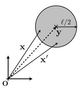
Figure 2: The voltage correlation function, $C({\bf x},{\bf x}^{\prime})$, is constructed by summing over all circular patches which contain both ${\bf x}$ and ${\bf x}^{\prime}$. This is undertaken by integrating over patch centers ${\bf y}$, and accounting for the distribution in patch sizes with the distribution $\Pi(\ell)$.

Given these considerations we find the following form for the correlation function:

$$C({\bf x},{\bf x}^{\prime}) =\int_{0}^{\infty}d\ell\ \Pi(\ell)$$

$$\times\frac{4V^{2}_{\mathrm{rms}}}{\pi\ell^{2}}\int d^{2}y\ \theta(\ell/2-|{\bf x}-{\bf y}|)\theta(\ell/2-|{\bf x}^{\prime}-{\bf y}|),$$

where the integral over $y$, constrained by the $\theta$-functions, sums over all patches of size $\ell$ which contain both points. The final integral over $\ell$ averages over patch sizes where $\Pi(\ell)$ is the distribution of patch diameters. Note in particular that the translational invariance of the correlation function is made apparent by the change of variables ${\bf x}^{\prime}-{\bf y}\to{\bf z}$ . Subsequently performing the integration over $y$ reveals the rotational invariance of the final result

$$C(r)\equiv C_{ii}(r) =\frac{2V^{2}_{\mathrm{rms}}}{\pi}\int_{r}^{\infty}d\ell\ \Pi(\ell)$$ (14)

$$\times\bigg{[}\cos^{-1}\left(\frac{r}{\ell}\right)-\frac{r}{\ell}\sqrt{1-\left(\frac{r}{\ell}\right)^{2}}\bigg{]}.$$

The patch power spectrum can then be obtained through the Fourier transform (II). Some interesting properties can be given at this point. First, the integration of the correlation function over all space is simply

$$C[k=0]=\frac{1}{4}\pi\overline{\ell^{2}}V^{2}_{\mathrm{rms}},$$ (15)

with $\overline{\ell^{2}}$ the variance of the distribution $\Pi(\ell)$. Second, the integral of $C[k]$ over wavevectors is just the variance of the potential $\int_{0}^{\infty}dkkC[k]=2\pi V^{2}_{\mathrm{rms}}$.

One can derive some universal scaling laws for the patch contribution to the pressure in some limiting cases. When the patches are much larger than the gap ($D\ll\bar{\ell}$), the expression (6) is obtained. This $1/D^{2}$ scaling law for the pressure (and the corresponding $1/D$ for the energy per unit area for planar plates) is universal for all patch power spectral densities whenever the typical patch sizes are much larger than the gap. In particular, this scaling was used in Sushkov11 to model the patch effect footnote . In the opposite limit, where the typical patch sizes are much smaller than the gap, one can obtain a simple scaling law. In this case the spectrum $C[k]$ is approximately constant over the wavevector range $k\stackrel{{\scriptstyle<}}{{\scriptscriptstyle{\sim}}}1/D$ which provides the most significant contribution to (II). We then find, when using (15),

$$P^{\mathrm{patch}}(D) \simeq \frac{\varepsilon_{0}}{2\pi}\,C[0]\,\int_{0}^{\infty}dk\,\frac{k^{3}}{{\rm sinh}^{2}(kD)}$$

$$\simeq \frac{3\zeta(3)}{4}\frac{\varepsilon_{0}V_{\mathrm{rms}}^{2}\overline{\ell^{2}}}{D^{4}}\approx 0.90\frac{\varepsilon_{0}V_{\mathrm{rms}}^{2}\overline{\ell^{2}}}{D^{4}}.$$

We emphasize at this point that this $1/D^{4}$ scaling law is generic for all spectra having a finite limit at $k=0$, but does not hold when $C[k]$ vanishes at $k=0$. In particular, in the model discussed in II-A, there is a sharp-cutoff of the power spectral density at $k_{\mathrm{min}}>0$. In this case, the pressure (II) is exponentially small when $k_{\mathrm{min}}D\gg 1$, that is also $D\gg\ell_{\mathrm{patch}}^{\mathrm{max}}$. The leading order contribution indeed comes from the exponential tail of $1/\sinh^{2}(kD)$ and is much smaller than the result found in the generic case (II.2). This point will play a crucial role in the comparison to experimental data discussed in the next section.

Before entering this discussion we choose a specific form for the patch size distribution $\Pi(\ell)$ which is similar in spirit to the sharp-cutoff model discussed in subsection II-A. By assuming the patch sizes are distributed uniformly within a finite interval between a minimum $\ell_{\mathrm{patch}}^{\mathrm{min}}$ and maximum $\ell_{\mathrm{patch}}^{\mathrm{max}}$ value, the probability distribution is

$$\Pi(\ell)=\frac{\theta(\ell_{\mathrm{patch}}^{\mathrm{max}}-\ell)\theta(\ell-\ell_{\mathrm{patch}}^{\mathrm{min}})}{\ell_{\mathrm{patch}}^{\mathrm{max}}-\ell_{\mathrm{patch}}^{\mathrm{min}}},$$ (17)

and has the following moments

$$\overline{\ell}=\frac{\ell_{\mathrm{patch}}^{\mathrm{max}}+\ell_{\mathrm{patch}}^{\mathrm{min}}}{2}$$ (18)

$$\overline{\ell^{2}}=\frac{(\ell_{\mathrm{patch}}^{\mathrm{max}})^{2}+(\ell_{\mathrm{patch}}^{\mathrm{min}})^{2}+\ell_{\mathrm{patch}}^{\mathrm{max}}\ell_{\mathrm{patch}}^{\mathrm{min}}}{3}.$$

Additionally, we would like to remark that we have also considered other size patch size distributions $\Pi(\ell)$ (log-normal, Gaussian, generalized gamma, etc.) and have found similar results for the pressure in all cases.

We emphasize that, despite some similarity in the construction of the two models discussed in subsections II-A and II-B, they correspond to very different correlation properties, the most striking difference resulting from a nonvanishing value for $C[k=0]$ in the quasi-local model which gives a distinct large distance behavior. In particular, a patch model employing quasi-local correlations was recently adopted to describe heating in ion traps and dissipation in cantilevers Dubessy09 . There, the observed large distance $(D\gg\overline{\ell})$ scaling of electric field noise ($\propto D^{-4}$) is linked with a nonvanishing value of $C[0]$.

To estimate the effects of contamination, we will assume that the patch power spectrum on a dirty surface takes the same form as on a clean surface (i.e., also given by the quasi-local model), with the exception that the parameters of the model are altered by the contaminants. Let us stress that quasi-local correlations may be not as accurate for contaminated surfaces as for clean ones. We employ the above assumptions in a preliminary manner to account for the properties of contaminated surfaces, to be confirmed by dedicated studies to come in the future.

III Comparison with experiments

We now compare the theory and experiments by calculating the Casimir force from the Drude model, and the patch pressure arising from the model with quasi-local correlations. To make the comparison we first calculate the plane-plane Casimir pressure $P_{pp}(D)$ at temperature $T$ using the Lifshitz formula Lifshitz ; Lambrecht00 ; Lambrecht06 . We use tabulated optical data for gold Palik , extrapolated to low frequencies with a Drude model to describe the contribution of conduction electrons, $\varepsilon_{\rm cond}(\omega)=1-\Omega_{P}^{2}/(\omega(\omega+i\gamma))$, where $\Omega_{P}$ is the plasma frequency and $\gamma$ quantifies the damping rate. To account for roughness corrections to the Casimir pressure we adopt the simplest formulation based on an additive scheme (Eq. (33) in Decca05 ). We will call the resulting pressure as the “Drude model” Casimir pressure $P_{pp}^{\rm Drude}(D)$.

As already stated, we use the PFA to relate the experimental data corresponding to the sphere-plane geometry to the predictions calculated in the plane-plane geometry, for the Casimir and the patch effects. In the IUPUI experiments the sphere-plane force gradient $G_{sp}$ is measured, which is related to the equivalent plane-plane pressure as in (1). In the Yale experiments the sphere-plane force $F_{sp}$ is measured, which is related similarly to the plane-plane energy per unit area.

After subtracting from the experimental data the theoretical predictions for the Casimir interaction, we find a residual signal

$$\delta{P}^{\rm Drude}(D)\equiv P^{\rm experiment}_{pp}(D)-P^{\rm Drude}_{pp}(D).$$ (19)

The question we address in the following is whether or not the residual $\delta{P}^{\rm Drude}$ can be explained by a reasonable modeling of patch effects. The criterium is then to minimize the remaining difference between the residual signal and the patch pressure $\delta{P}^{\rm Drude}(D)-P^{\mathrm{patch}}(D)$. The residual is defined here for the Drude model and may be as well be defined for the plasma model. The patch pressure $P^{\mathrm{patch}}(D)$ is then defined for a given patch model, say in particular the sharp-cutoff (subsection II-A) or quasi-local (subsection II-B) models.

III.1 Data analysis for the IUPUI experiment

For the comparison with the IUPUI experiment we compute the Casimir force at room temperature $T=295$ K using tabulated optical data extrapolated to low frequencies with a Drude model with parameters $\Omega_{P}=8.9$ eV for the plasma frequency and $\gamma=0.0357$ eV for the damping rate. Root mean square roughness heights for the plane and the sphere are $3.6$ nm and $1.9$ nm, respectively. These permittivity and roughness parameters are the ones reported in Decca07 .

We collect in Fig.3 the information needed to compare IUPUI experimental data with predictions from the Drude model and modelings of the patch effect. We plot the residuals $\delta{P}^{\rm Drude}$ defined as in (19) as points with error bars and the patch pressure $P_{\mathrm{patch}}$ for different patch models as lines. The error bars represent the total experimental error described in Fig. 2 of Decca07 at $67\%$ confidence. The theoretical predictions for the Casimir pressure $P_{pp}^{\rm Drude}$ are calculated for the Drude model as described above and assumed to have no error. There are four different patch models represented in Fig.3 :

1. The solid curve is the estimation of the patch effect using all the assumptions of subsection II-A. The patches are thus described by the sharp-cutoff model (8) with the parameters $k_{\mathrm{max}}=251\,\mu\mathrm{m}^{-1}$, $k_{\mathrm{min}}=20.9\,\mu\mathrm{m}^{-1}$ and $V_{\mathrm{rms}}=80.8$ mV (these are the parameters used in Decca05 ).

2. The dotted curve is the result of the quasi-local correlation model (14) with the patch size distribution (17) described in subsection II-B. The parameters, $\ell_{\mathrm{patch}}^{\mathrm{min}}=25$nm, $\ell_{\mathrm{patch}}^{\mathrm{max}}=300$nm and $V_{\mathrm{rms}}=80.8$ mV, correspond to the assumptions that the patch sizes are given by the grain sizes and the rms voltage is determined by the variance of the work function over the different crystallographic planes (these are the same parameters used in item 1 above).

3. The long-dashed curve is obtained from a least-squares minimization of the difference $\delta{P}^{\rm Drude}(D)-P^{\mathrm{patch}}(D)$, using the quasi-local patch correlation model given by (14) and (17). As $\ell_{\mathrm{patch}}^{\mathrm{min}}$ is found to have a small influence, we fix it to the smallest grain size $\ell_{\mathrm{patch}}^{\mathrm{min}}=25$ nm as discussed above. The best fit on the two remaining parameters gives $\ell_{\mathrm{patch}}^{\mathrm{max}}\approx 2476$ nm and $V_{\mathrm{rms}}\approx 9.2$ mV and results in qualitative agreement between the residual and the fitted patch pressure. The associated first moments of the patch size distribution are $\overline{\ell}=1251$ nm and $\overline{\ell^{2}}=(1437$ nm$)^{2}$. The reduced-$\chi^{2}$ for this fit, calculated using the total error bars from Fig 2. of Decca07 at $67\%$, is $0.814$. It is important to note that the values of the fit parameters and quality of the fit are very sensitive to the sample’s optical parameters, in particular to the plasma frequency used in the extrapolation of optical data to low frequencies sampledep . However, one should avoid giving too much importance to any of these values of reduced-$\chi^{2}$ as a measure with statistical significance of experiment-theory agreement. Indeed, the influence of sample dependency of optical parameters, the use of a very crude description of roughness corrections to the Casimir pressure, and, most importantly, the lack of precise information of the patch correlation function in actual experimental samples, all imply that the fits obtained with the quasi-local model for patches have a qualitative nature; dedicated patch effects measurements are required to make metrological claims (see the Conclusions for further discussions).

4. The short-dashed curve (underneath the long-dashed curve) is a fit of a phenomenological model proposed by Carter and Martin Carter11 . The correlation function of this model, based on a Monte-Carlo simulation of patch layouts, can be expressed in terms of a shifted Gaussian and is specified by the rms voltage and the average patch area $w^{2}$, related to our patch radius via $w\approx\sqrt{\pi}\,\,\overline{\ell}/2$. Our best fit values are $\overline{\ell}\approx 1229$ nm and $V_{\mathrm{rms}}=8.6$ mV with reduced-$\chi^{2}$ of 0.812.

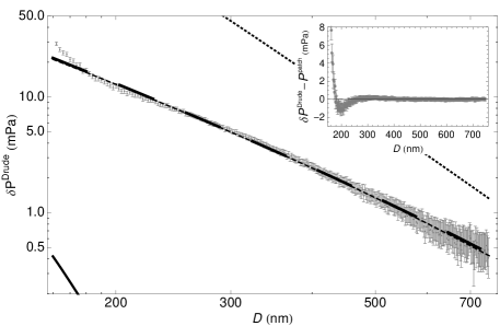
Figure 3: Comparison of the residual $\delta{P}^{\rm Drude}$ between the experimental pressure in Decca07 and the Drude prediction (points with error bars at $67\%$ confidence taken from Fig. 2 of Decca07 ) with patch pressure $P_{\mathrm{patch}}$ for four different patch models (more details in the main text) : 1. The solid curve is the result of the sharp-cutoff model (with assumptions of subsection II-A) ; 2. The dotted curve corresponds to the quasi-local patch correlation model assuming that the patch sizes are given by the grain sizes and that the rms voltage is given by the variance of the work function over different crystallographic planes ; 3. The long-dashed curve is the result of a best-fit on the parameters ($\ell_{\mathrm{max}}$ and $V_{\mathrm{rms}}$) of the quasi-local patch correlation model ; 4. The short-dashed curve (underneath the long-dashed curve) is a fit of a phenomenological model proposed in Carter11 . The inset shows the residual signal resulting from subtracting the fit of the quasi-local model (long-dashed curve) from $\delta P^{\rm Drude}$.

After this description of the information gathered on Fig. 3, let us now comment on the significance of the various results:

1. The solid curve reproduces and confirms the calculations which were performed to quantify patch effects in Decca05 ; Decca07 . With the assumptions described in subsection II-A, the calculated patch pressure is indeed far too small to explain the difference between experimental data and theoretical predictions using the Drude model.

2. The dotted curve gives the result of the quasi-local model of patch correlations (17) with parameters determined as was done in Decca05 ; Decca07 , but here for a different patch spectrum model. As a striking illustration of the importance of this difference, the calculated patch pressure is now larger than the difference between experimental data and theoretical predictions using the Drude model. This illustrates the highly model dependent nature of the computed patch pressure. Thus, patches may be an important systematic effect for which their contribution to the measured signal should ideally be assessed independently of any Casimir force measurement.

3. The long-dashed curve corresponds to a least squares fit of the quasi-local correlation model to the residual $\delta P^{\rm Drude}$. With the best-fit parameters $\ell_{\mathrm{patch}}^{\mathrm{max}}$ and $V_{\mathrm{rms}}$, this model qualitatively fits the difference between experimental data and theoretical predictions using the Drude model. These parameters have reasonable values: $\ell_{\mathrm{patch}}^{\mathrm{max}}$ is larger than the maximum grain size on the samples, and $V_{\mathrm{rms}}$ smaller than the rms voltage for a clean sample Decca05 ; Decca07 . This suggests the presence of contaminants on the sample surfaces Rossi92 .

4. The best-fit of the phenomenological model proposed in Carter11 is essentially indistinguishable from that of the quasi-local correlation model (long-dashed curve). The best-fit values for $\overline{\ell}$ and $V_{\mathrm{rms}}$ are consistent with the average patch size and rms voltage obtained from the best-fit parameters of the quasi-local model.

At this point, we also want to comment on the validity requirement (7), which allows one to calculate the patch effect in the sphere-plane geometry within the PFA. This requirement ensures that the effective area of interaction between the sphere and the plane, of the order of $\pi RD$ for a sphere of radius $R$, contains a large number of elementary patch areas, so that the sum over the micro-realization of patches on a given plate is a good effective description of the statistical ensemble-average given by the power spectral density. With the numbers in Decca07 , that is a radius of curvature of the sphere $R=151.3\mu$m and a shortest distance $D_{\mathrm{min}}=160$nm, the interaction area is $\pi RD\approx 76(\mu\text{m})^{2}$. Meanwhile, the average patch area is $(\pi/4)\overline{\ell^{2}}\approx 1.6(\mu\text{m})^{2}$, there is a large number of elementary patch areas ($\approx 48$) within the effective area of interaction, but it is possible that one could expect a small correction to the patch pressure at short distances when the ergodic hypothesis begins to break down.

For completeness we have also studied the residual $\delta P^{\rm plasma}(D)$, as defined in Eq. (19), with the exception that we have compute the plane-plane Casimir pressure $P_{pp}^{\rm plasma}(D)$ using the “plasma model”, instead of the Drude model. More precisely, we have computed the pressure using for the permittivity $\varepsilon(i\xi)$ the “generalized plasma model”:

$$\varepsilon^{\rm g.plasma}(i\xi)=1+\frac{\Omega^{2}_{P}}{\xi^{2}}+\sum_{j=1}^{6}\frac{f_{j}}{\omega_{j}^{2}+\xi g_{j}+\xi^{2}},$$ (20)

where the first two terms correspond to the permittivity for the plasma model for conduction electrons (dissipation of conduction electrons is set to zero ad hoc without physical justification), and the second sum of terms accounts for the interband transitions of gold parameters . To account for roughness corrections to the Casimir pressure we use the same additive scheme employed above. Computing $\delta P^{\rm plasma}(D)$ in this way, we have confirmed the findings of Decca05 ; Decca07 , namely that a negligible contribution of the patch effect leads to an agreement of data with theoretical predictions using the plasma model. We note, however, that the patch pressure calculated from the quasi-local model, with sizes and voltages used in Decca05 , is much larger than the difference between the measurements and the plasma prediction, as shown in Fig. 4 footnote2 . We think that this result constitutes a serious warning against the claims according to which the plasma model would be confirmed with a high confidence level by Casimir experiments performed with real metals Klimchitskaya09 .

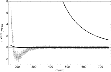
Figure 4: Comparison of the residual $\delta{P}^{\rm plasma}$ (points with error bars at $67\%$ confidence taken from Fig. 2 of Decca07 ) with patch pressures given by the sharp-cutoff model and the quasi-local model: 1. The solid curve is the result of the sharp-cutoff model (with assumptions of subsection II-A). We find, consistently with the analysis in Decca05 ; Decca07 , that the patch pressure from this model gives a negligible contribution to the measured signal. 2. The dotted curve corresponds to the quasi-local patch correlation model adopting the same parameters used in Decca05 ; Decca07 for the patch size and the rms voltage. In distinction to the sharp-cutoff model, we find that the quasi-local model gives a large signal as compared to the residual $\delta{P}^{\rm plasma}$.

III.2 Data analysis for the Yale experiment

In addition to analyzing the IUPUI experiment we now apply the same models to the recent experiment by the Yale group Sushkov11 . A patch analysis was already carried out in Sushkov11 and it led to a good agreement between experimental data and the Drude model. This analysis only considered the asymptotic form $\propto 1/D$ of the plane-plane energy due to patches (6). Here we extend the analysis by using the more general expression (II) for the patch pressure with the quasi-local patch correlation function described in subsection II-B. Because we have no information regarding grain or patch sizes in the Yale experiment, we will focus our attention on best-fit estimations of the parameters $\ell^{\rm max}_{\rm patch}$, $\ell^{\rm min}_{\rm patch}$, and $V_{\rm rms}$ characterizing the quasi-local patch correlation function (14,17).

To analyze Yale experimental data we first compute the Casimir force using tabulated optical data extrapolated to low frequencies with the Drude model using the plasma frequency $\Omega_{P}=7.54$ eV and the dissipation rate $\gamma=0.052$ eV employed in Sushkov11 . We set the temperature to be $T=295$K. The roughness correction to the Casimir force is ignored as it gives a negligible correction to the force at the distances considered in the Yale experiment. Fig.5 shows the difference of the Yale experimental force data and the Casimir force prediction using the Drude model, $\delta F^{\rm Drude}$ (defined by analogy with (19)), depicted by points with error bars (we assume no error for the theory). The solid curve shows the resulting patch force for parameters arising from a least-squares minimization of the quantity $\delta F^{\rm Drude}-F^{\mathrm{patch}}$ using the quasi-local patch correlation model (17) described in subsection II-B. The best fit parameters are given by $\ell_{\mathrm{patch}}^{\mathrm{max}}\approx 614\mu$m, $\ell_{\mathrm{patch}}^{\mathrm{min}}\approx 566\mu$m, (corresponding with $\overline{\ell}=590\mu$m) and $V_{\mathrm{rms}}\approx 3.9$ mV. We should point out, however, that the result of the best-fit is essentially insensitive to the details of the patch power spectrum. Indeed, since the residual $\delta P^{\rm Drude}$ in the Yale experiment has an approximate $1/D$ power law we can infer using (6) that the typical patch size is much larger than $D$ for the whole range of distances explored in the experiment (0.7 $\mu$m - 7$\mu$m). Performing a constrained fitting by requiring that $\ell^{\rm max}_{\rm patch}$ be less than some predetermined value (e.g. 500 $\mu$m), yet still satisfying the constraint $\bar{\ell}\gg D$, we were able to verify that a good fit can still be achieved over a large range of patch sizes. In summary, we point out the result of our fitting using the more detailed quasi-local patch model confirms the patch treatment in Sushkov11 .

Figure 5: Comparison of the residual $\delta F^{\rm Drude}$ between the data of Sushkov11 and the computed sphere-plane force with the associated patch pressure $F^{\mathrm{patch}}$. The dots correspond to $\delta F^{\rm Drude}$, with the errors bars including only the experimental error in the force determination. The solid line is a best-fit of the patch force within the quasi-local model of subsection II-B. The inset shows the corresponding residual $\delta F^{\rm plasma}$ with the same convention employed in the main figure.

Finally, we also report for the sake of completeness some supplementary test we performed for comparing the data in Sushkov11 with the predictions of the plasma model described by Eq.(20) (see the inset of Fig. 5). The good agreement obtained for the Drude model is dramatically degraded. Therefore, we confirm the result obtained in Sushkov11 that patches cannot explain the difference between the experimental data and the plasma model in Yale data.

IV Concluding Remarks

In this paper, we have analyzed the patch contribution to Casimir experiments with a model featuring quasi-local voltage correlations. Our model is derived from well-motivated physical principles and shares key features with experimentally verified patch models used to describe ion trap heating and cantilever damping Dubessy09 . Thus, for the description of the surfaces used in the experiments discussed in this paper, we believe that this model is more appropriate than the sharp-cutoff model which has been used to the same aim in previous publications Decca05 ; Decca07 .

Due to the large difference in the patch power spectrum, in particular for small wavevectors, the quasi-local model gives a larger contribution than the sharp-cutoff model. As a striking consequence, when the patch sizes are deduced from the grain sizes (as was done in Decca05 ; Decca07 ), the quasi-local model produces a patch pressure larger than the difference between the experimental data and the Drude (and plasma) Casimir prediction, whereas the sharp-cutoff model produces a negligible patch pressure. Therefore, it is important to emphasize that because of the combination of: a) the highly model dependent nature of the computed patch pressure and b) the potentially large patch contribution to the measured signal, patches may lead to nonnegligible systematic effects. This necessitates an independent measurement of patch effects in order to meet metrological standards for Casimir force measurements.

We have also used the new quasi-local patch model to fit the difference between experimental data of the IUPUI experiment Decca05 ; Decca07 and the theoretical prediction for the Casimir pressure. The latter was computed taking into a) tabulated optical data extrapolated to low frequencies by means of the Drude model, and b) roughness effects modeled by a simple additive technique. We have found best-fit parameters for the average patch size and for the rms voltage that are consistent with a contamination of the metallic surfaces, which is expected to enlarge the patch sizes (with respect to grain sizes) and smear the patch voltage (with respect to those of a surface of bare crystallites) Rossi92 . Indeed, surface contamination is expected, and we believe that preferential adsorption Rossi92 and saturation of contaminants may be compatible with the observation of reproducible results in experiments repeated several times with different samples DeccaPC .

Taken together, our results constitute a strong warning against the previously published claims of an agreement of Casimir experiments with the plasma model, and an elimination of the Drude model Klimchitskaya09 . However, we want to emphasize that they do not constitute yet a proof of agreement of experimental data with the new model. The parameters of the patch model have been fitted and it is still possible that the qualitative agreement thus obtained is a fortunate output of the fitting procedure rather than an explanation of the experimental data.

In this paper we have focused our attention on only the IUPUI and Yale experiments, but of course the analysis can be repeated for other Casimir measurements between metallic plates as well Chan01 ; Bressi02 ; Chen04 ; Lisanti05 ; Svetovoy08 ; Onofrio08 ; Jourdan09 ; deMan09 ; Masuda09 ; Antonini09 .

A better characterization of the surfaces used in the experiments is now key to reaching firmer conclusions. The patch distributions can be measured with appropriate technologies such as Kelvin probe force microscopy which can achieve the necessary size and voltage resolutions Liscio08 ; Liscio11 . In addition, the study of cold atoms and cold ions trapped in the vicinity of metallic surfaces Epstein07 or the role of patch effects in other precision measurements Adelberger09 ; Everitt11 ; Reasenberg11 are other ways for accessing information of interest for our problem. Let us repeat at this point that our new quasi-local model is similar to recent proposals for patch physics used to achieve a better understanding of atomic and ionic traps Dubessy09 ; Carter11 .

The challenges of forthcoming studies may be stated as follows. First, it is important to confirm the hypothesis that the patch voltages show quasi-local correlations, and to better specify the power spectrum which quantitatively describes these correlations. Second, it would also be interesting to study how the patch power spectrum depends on contamination, in particular, fabrication, treatment, history of the samples, and on temperature. Finally, an independent determination of the patch power spectrum could lead either to a confirmation of the best-fit analysis presented in this paper or to new questions. This study is important not only for the test of the Casimir effect, a central prediction of quantum field theory, but also for the searches of the hypothetical new short-range forces predicted by unification models Fischbach98 ; Adelberger03 ; Onofrio06 ; Antoniadis11 .

- (1) H. B. G. Casimir, Proc. Kon. Ned. Akad. Wetensch. 51, 793 (1948).
- (2) S. K. Lamoreaux, Rep. Prog. Phys. 60, 201 (2005).
- (3) M. Bordag, G. L. Klimchitskaya, U. Mohideen and V. M. Mostepanenko, Advances in the Casimir Effect (Oxford University Press, Oxford, 2009).
- (4) D. A. R. Dalvit, P. Milonni, D. Roberts and F. S. da Rosa (editors), Casimir Physics (Lecture Notes in Physics 834) (Springer-Verlag, Heidelberg, 2011).
- (5) E. Fischbach and C. Talmadge, The Search for Non Newtonian Gravity (AIP Press/Springer Verlag, 1998).
- (6) E.G. Adelberger, B.R. Heckel and A.E. Nelson, Ann. Rev. Nucl. Part. Sci. 53, 77 (2003).
- (7) R. Onofrio, New J. Phys. 8, 237 (2006).
- (8) I. Antoniadis, S. Baessler, M. Büchner et al, Compt. Rend. Acad. Sci. to appear (2011).
- (9) R.S. Decca, D. López, E. Fischbach et al, Annals Phys. 318, 37 (2005).
- (10) R.S. Decca, D. López, E. Fischbach et al, Phys. Rev. D 75, 077101 (2007).
- (11) A.O. Sushkov, W.J. Kim, D.A.R. Dalvit and S.K. Lamoreaux, Nat. Phys. 7, 230 (2011).
- (12) C.C. Speake and C. Trenkel, Phys. Rev. Lett. 90, 160403 (2003).
- (13) A.A. Chumak, P.W. Milonni and G.P. Berman, Phys. Rev. B 70, 085407 (2004).
- (14) W.J. Kim, A.O. Sushkov, D.A.R. Dalvit and S.K. Lamoreaux, Phys. Rev. A 81, 022505 (2010).
- (15) S. de Man, K. Heeck, R.J. Wijngaarden and D. Iannuzzi, J. Vac. Sci. Technol. B 28, C4A25 (2010).
- (16) W. J. Kim and U. Schwarz, C4A1 J. Vac. Sci. Technol. B 28, 3 (2010).
- (17) F. C. Witteborn and W. M. Fairbank, Phys. Rev. Lett. 19, 1049 (1967).
- (18) J.B. Camp, T.W. Darling and R.E. Brown, J. Appl. Phys. 69, 7126 (1991).
- (19) Q.A. Turchette, D. Kielpinski, B.E. King et al, Phys. Rev. A 61, 063418 (2000).
- (20) L. Deslauriers, S. Olmschenk, D. Stick et al, Phys. Rev. Lett. 97,103007 (2006).
- (21) N.A. Robertson, J.R. Blackwood, S. Buchman et al, Class. Quantum Grav. 23, 2665 (2006).
- (22) R.J. Epstein, S. Seidelin, D. Leibfried et al, Phys. Rev. A 76, 033411 (2007).
- (23) S.E. Pollack, S. Schlamminger and J.H. Gundlach, Phys. Rev. Lett. 101, 071101 (2008).
- (24) E.G. Adelberger, J.H. Gundlach, B.R. Heckel, S. Hoedl and S. Schlamminger, Progr. Particle Nuclear Phys. 62, 102 (2009).
- (25) C.W.F. Everitt, D.B. DeBra, B.W. Parkinson et al, Phys. Rev. Lett. 106, 221101 (2011).
- (26) R.D. Reasenberg, E.C. Lorenzini, B.R. Patla et al, Class. Quantum Grav. 28, 094014 (2011).
- (27) N. Gaillard et al, Appl. Phys. Lett. 89, 154101 (2006).
- (28) F. Rossi and G. I. Opat, J. Appl. Phys. D 25, 1349 (1992).
- (29) A. Naji, D.S. Dean, J. Sarabadani, R.R. Horgan and R. Podgornik, Phys. Rev. Lett. 104, 060601 (2010).
- (30) J. Sarabadani, A. Naji, D. S. Dean, R. Horgan, and R. Podgornik, J. Chem. Phys. 133, 174702 (2010).
- (31) R. Dubessy, T. Coudreau, and L. Guidoni, Phys. Rev. A 80, 031402 (2009).
- (32) J.D. Carter and J.D.D. Martin, Phys. Rev. A 83, 032902 (2011).
- (33) I. S. Gradshteyn and I. M. Ryzhik, Table of Integrals, Series, and Products (Academic Press, London, 1994).
- (34) As a minor remark, we should point out that the definitions of used here and in Sushkov11 differ by a factor .
- (35) E. M. Lifshitz, Sov. Phys. JETP 2, 73 (1956).
- (36) A. Lambrecht and S. Reynaud, Euro. Phys. J. D 8, 309 (2000).
- (37) A. Lambrecht, P.A. Maia Neto and S. Reynaud, New J. Phys. 8, 243 (2006).
- (38) E. D. Palik (ed.), Handbook of Optical Constants of Solids, (Academic, New York, 1985).
- (39) We performed the same fitting procedure for eV and eV (keeping and the roughness model and parameters fixed), and found nm, mV, reduced- , and nm, mV, reduced- , respectively.
- (40) The values of the interband parameters used in Eq.(20) are: , , ; , , ; , , ; , , ; , , ; and , , . Units of and are eV, units of are .
- (41) See for example V. A. Parsegian and G. H. Weiss, J. Coll. Int. Sci. 81, 285 (1981).
- (42) The quasi-local model can also be fitted to the residual , but, not surprisingly, the fit is insensitive to patch sizes as the residual signal is compatible with 0 over a large range, implying .
- (43) Ricardo Decca (private communication).
- (44) G.L. Klimchitskaya, U. Mohideen and V.M. Mostepanenko, Rev. Mod. Phys. 81, 1827 (2009).
- (45) H. B. Chan, V. A. Aksyuk, R. N. Kleiman, D. J. Bishop and F. Capasso, Phys. Rev. Lett. 87, 211801 (2001).
- (46) G. Bressi, G. Carugno, R. Onofrio and G. Ruoso, Phys. Rev. Lett. 88, 041804 (2002).
- (47) F. Chen, G.L. Klimchitskaya, U. Mohideen and V.M. Mostepanenko, Phys. Rev. A 69, 022117 (2004).
- (48) M. Lisanti, D. Iannuzzi and F. Capasso, Proc. Nat. Ac. Sci. USA 102, 11989 (2005).
- (49) V.B. Svetovoy, P.J. van Zwol, G. Palasantzas and J.Th.M. De Hosson, Phys. Rev. B 77, 035439 (2008).
- (50) W. J. Kim, M. Brown-Hayes, D. A. R Dalvit, J. H. Brownell and R. Onofrio, Phys. Rev. A 78, 020101(R) (2008).
- (51) G. Jourdan, A. Lambrecht, F. Comin and J. Chevrier, Euro. Phys. Lett. 85, 31001 (2009).
- (52) S. de Man, K. Heeck and D. Iannuzzi, Phys. Rev. A 79, 024102 (2009).
- (53) M. Masuda and M. Sasaki, Phys. Rev. Lett. 102, 171101 (2009).
- (54) P. Antonini, G. Bimonte, G. Bressi, G. Carugno, G. Galeazzi, G. Messineo and G. Ruoso, J. Phys. Conf. Ser. 161, 012006 (2009).
- (55) A. Liscio, V. Palermo, K. Müllen and P. Samori, J. Phys. Chem. C 112, 17368 (2008).
- (56) A. Liscio, V. Palermo and P. Samori, Accounts Chem. Res. 43, 541 (2010).