Graphene Simulation Graphene and Cousin Systems Graphene and Cousin Systems Morocco

1 Introduction

Besides its simple molecular structure, the magic of 2D graphene, a sheet of carbon graphite, is essentially due to two fundamental electronic properties: First for its peculiar band structure where valence and conducting bands intersect at two points $K_{+}$ and $K_{-}$ of the reciprocal space of the 2D honeycomb making of graphene a zero gap semi-conductor. Second, for the ultra relativistic behavior of the charge carriers near the Fermi level where the energy dispersion relation $E=E\left(p\right)$ behaves as a linear function in momenta; $E\left(p\right)=v_{f}p+O\left(p^{2}\right)$. This typical property, which is valid for particles with velocity comparable to the speed of light, was completely unexpected in material science and was never suspected before 2004; the year where a sheet of 2D graphene has been experimentally isolated (Novoselov et al.,, 2004; Geim & Novoselov,, 2007). From this viewpoint, graphene is then a new material with exotic properties that could play a basic role in the engineering of electronic devices with high performances; it also offers a unique opportunity to explore the interface between condensed interface between condensed matter physics and relativistic Dirac theory where basic properties like chirality can be tested; and where some specific features, such as numerical simulation methods, can be mapped to 4D lattice gauge theory like lattice QCD (Creutz,, 2008; Boriçi,, 2008; Capitani et al.,, 2010). Although looking an unrealistic matter system, interest into the physical properties of graphene has been manifested several decades ago. The first model to analyze the band structure of graphite in absence of external fields was developed by Wallace in 1947 (Wallace,, 1947); see also (Slonczewski & Weiss,, 1958). Since then, several theoretical studies have been performed on graphene in the presence of a magnetic field (Haldane,, 1983)-(Goerbig et al.,, 2006). The link between the electronic properties of graphene and $\left(2+1\right)$-dimensional Dirac theory was also considered in many occasions; in particular by Semenoff, Fradkin and Haldane during the 80-th of the last century (Semenoff,, 1984; Haldane,, 1988; Castro-Neto et al.,, 2009); see also (Jackiw & Pi,, 2007, 2008) and refs therein.
In this book chapter, we use the tight binding model as well as the ${SU}\left({3}\right)$ hidden symmetry of 2D honeycomb to study some physical aspects of 2D graphene with a special focus on the electronic properties. We also develop new tools to study some of graphene’s cousin systems such as the 1D- poly-acetylene chain, cumulene, poly-yne, Kekulé cycles, the 3D diamond and the 4D hyperdiamond models. As another application of the physics in higher dimension, we also develop the relation between the so called four dimensional graphene first studied in (Creutz,, 2008; Drissi et al., 2011 a, ; Bedaque et al.,, 2008); and 4D lattice quantum chromodynamics (QCD) model considered recently in the lattice quantum field theory (QFT) literature to deal with QCD numerical simulations (Capitani et al., 2009 a, ; Capitani et al., 2009 b, ).
The presentation is as follows: In section 2, we review the main lines of the electronic properties of 2D graphene and show, amongst others, that they are mainly captured by the $SU(3)$ symmetry of the 2D honeycomb. In section 3, we study higher dimensional graphene type systems by using the power of the hidden symmetries of the underlying lattices. In section 4, we give four examples of graphene’s derivatives namely the 1D- poly-acetylene chain, having a $SU(2)$ invariance, as well as Kekulé cycles thought of as a particular 1D- system. We also study the 3D diamond model which exhibits a $SU\left(4\right)$ symmetry; the corresponding 2D model, with $SU(3)$ invariance, is precisely the graphene considered in section 2. In section 5, we develop the four dimensional graphene model living on the 4D hyperdiamond lattice with a SU$\left(5\right)$ symmetry. In section 6, we study an application of this method in the framework of 4D lattice QCD. Last section is devoted to conclusion and comments.

2 Two dimensional graphene

First, we give a brief review on the tight binding modeling the physics of 2D graphene; then we study its electronic properties by using hidden symmetries. We show amongst others that the 2D honeycomb is precisely the weight lattice of $SU\left(3\right)$ (Drissi et al.,, 2010); and the two Dirac points are given by the roots of $SU\left(3\right)$. This study may be also viewed as a first step towards building graphene type systems in diverse dimensions.

2.1 Tight binding model

Graphene is a two dimensional matter system of carbon atoms in the $sp^{2}$ hybridization forming a 2D honeycomb lattice. This is a planar system made of two triangular sublattices $\mathcal{A}_{2}$ and $\mathcal{B}_{2}$; and constitutes the building block of the layered 3D carbon graphite. Since its experimental evidence in 2004, the study of the electronic properties of graphene with and without external fields has been a big subject of interest; some of its main physical aspects were reviewed in (Castro-Neto et al.,, 2009) and refs therein. This big attention paid to the 2D graphene, its derivatives and its homologues is because they offer a real alternative for silicon based technology and bring together issues from condensed matter and high energy physics (Giuliani et al.,, 2010)-Chakrabarti et al., (2009) allowing a better understanding of the electronic band structure as well as their special properties.
In this section, we focus on a less explored issue of 2D graphene by studying the link between specific electronic properties and a class of hidden symmetries of the 2D honeycomb. These symmetries allow to get more insight into the transport property of the electronic wave modes and may be used to approach the defects and the boundaries introduced in the graphene monolayer (Cortijo & Vozmediano,, 2009). The existence of these hidden symmetries; in particular the remarkable hidden $SU\left(3\right)$ invariance considered in this study, may be motivated from several views. For instance from the structure of the first nearest carbon neighbors like for the typical $\left\langle A_{0}\text{-}B_{1}\right\rangle$, $\left\langle A_{0}\text{-}B_{2}\right\rangle,$ $\left\langle A_{0}\text{-}B_{3}\right\rangle$ as depicted in triangle of fig(1).

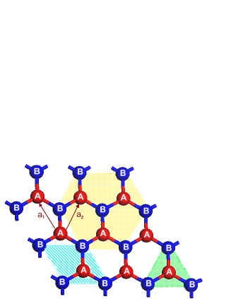
Figure 1: Sublattices A and B of the honeycomb with unit cell given by dashed area. A-type carbons are given by red balls and B-type atoms by blue ones. Each carbon has three first nearest neighbors as shown by the triangle; and six second nearest ones.

These doublets $A_{0}$-$B_{1}$, $A_{0}$-$B_{2},$ $A_{0}$-$B_{3}$ are basic patterns generating the three $SU\left(2\right)$ symmetries contained in the hidden $SU\left(3\right)$ invariance of honeycomb. The $A$-$B$ patterns transform in the isospin $\frac{1}{2}$ representations of $SU\left(2\right)$ and describe the electronic wave doublets $\phi_{{\scriptsize\pm}\frac{{\scriptsize 1}}{{\scriptsize 2}}}=\left[a\left(\mathbf{r}\right),b\left(\mathbf{r}\right)\right]$ interpreted as quasi-relativistic 2D spinors in the nearby of the Dirac points (Castro-Neto et al.,, 2009). The $SU\left(3\right)$ hidden symmetry of honeycomb is also encoded in the second nearest neighbors $\left\langle\left\langle A_{0}\text{-}A_{i}\right\rangle\right\rangle$ and $\left\langle\left\langle B_{0}\text{-}B_{i}\right\rangle\right\rangle,$ $i=1,...,6$ which capture data on its adjoint representation where the six $\left\langle\left\langle A_{0}\text{-}A_{i}\right\rangle\right\rangle$ (and similarly for $\left\langle\left\langle B_{0}\text{-}B_{i}\right\rangle\right\rangle$) are precisely associated with the six roots of $SU\left(3\right)$ namely $\pm\mathbf{\alpha}_{1},$ $\pm\mathbf{\alpha}_{2},$ $\pm\mathbf{\alpha}_{3}$; see below. In addition to above mentioned properties, hidden symmetries of graphene are also present in the framework of the tight binding model with hamiltonian,

$$H=$$ ,

(2.1)

where $t\simeq 2.8eV$ is the hopping energy; and where the fermionic creation and annihilation operators $a,$ $b,$ $a^{\dagger},$ $b^{\dagger}$ are respectively associated to the pi-electrons of each atom of the sublattices $\mathcal{A}_{2}$ and $\mathcal{B}_{2}$. The three relative vectors $\mathbf{v}_{1}$, $\mathbf{v}_{2}$, $\mathbf{v}_{3}$ define the first nearest neighbors, see fig(2) for illustration. These 2D vectors are globally defined on the honeycomb and obey the remarkable constraint equation

$$\mathbf{v}_{1}+\mathbf{v}_{2}+\mathbf{v}_{3}=\mathbf{0,}$$ (2.2)

which, a priori, encodes also information on the electronic properties of graphene. Throughout this study, we show amongst others, that the three above mentioned $SU\left(2\right)$’s are intimately related with these $\mathbf{v}_{n}$’s which, as we will see, are nothing but the weight vectors $\mathbf{\lambda}_{n}$ of the $SU\left(3\right)$ symmetry; i.e $\mathbf{v}_{n}=a\frac{\mathbf{\lambda}_{n}}{\left\|\mathbf{\lambda}_{n}\right\|}$. The wave functions $\phi_{\mathbf{\lambda}_{n}}\left(\mathbf{r}\right)$ of the delocalized electrons are organized into a complex $SU\left(3\right)$ triplet of waves as given below

$$\left(\begin{array}[]{c}\left|\mathbf{\lambda}_{1}\right\rangle\\ \left|\mathbf{\lambda}_{2}\right\rangle\\ \left|\mathbf{\lambda}_{3}\right\rangle\end{array}\right)\equiv\underline{\mathbf{3}}$$

(2.3)

The symbol $\underline{\mathbf{3}}$ refers to the 3-dimensional representation of $SU\left(3\right)$; say with dominant weight $\mathbf{\lambda}_{1}$. We also show that the mapping of the condition $\sum_{n=1}^{3}\mathbf{\lambda}_{n}=\mathbf{0}$ to the momentum space can be interpreted as a condition on the conservation of total momenta at each site of honeycomb. This connection with $SU\left(3\right)$ representations opens a window for more insight into the study of the electronic correlations in 2D graphene and its cousin systems by using symmetries.
The organization of this section is as follows: In subsection 2, we exhibit the $SU\left(3\right)$ symmetry of graphene. We also give a field theoretic interpretation of the geometric constraint equation $\mathbf{v}_{1}+\mathbf{v}_{2}+\mathbf{v}_{3}=\mathbf{0}$ both in real and reciprocal honeycomb. We also use the simple roots and the fundamental weights of hidden $SU\left(3\right)$ symmetry to study aspects of the electronic properties of 2D graphene. In subsection 3, we develop the relation between the energy dispersion relation $E\left(k_{x},k_{y}\right)$ and the hidden $SU\left(3\right)$ symmetry. Comments regarding the link between graphene bilayers and symmetries are also given.

2.2 Symmetries and electronic properties

2.2.1 Hidden symmetries of graphene

In dealing with pristine 2D graphene, one immediately notices the existence of a hidden $SU\left(3\right)$ group symmetry underlying the crystallographic structure of the honeycomb lattice and governing the hopping of the pi-electrons between the closed neighboring carbons. To exhibit this hidden $SU\left(3\right)$ symmetry, let us start by examining some remarkable features on the graphene lattice and show how they are closely related to SU$\left(3\right)$. Refereing to the two sublattices of the graphene monolayer by the usual letters $\mathcal{A}_{2}$ and $\mathcal{B}_{2}$ generated by the vectors $\mathbf{a}_{1}=d(\sqrt{3},0),$ $\mathbf{a}_{2}=\frac{d}{2}(-\sqrt{3},3)$; together with the three relative $\mathbf{v}_{1}=\frac{d}{2}(\sqrt{3},1),$ $\mathbf{v}_{2}=\frac{d}{2}(-\sqrt{3},1),$ $\mathbf{v}_{3}=-\mathbf{v}_{1}-\mathbf{v}_{2}$ with carbon-carbon distance $d\simeq 1.42$ $A^{\textdegree}$; and denoting by $\phi_{A}\left(\mathbf{r}_{i}\right)$ and $\phi_{B}\left(\mathbf{r}_{j}\right)$ the wave functions of the corresponding pi-electrons, one notes that the interactions between the first nearest atoms involve two kinds of trivalent vertices capturing data on $SU\left(3\right)$ symmetry, see fig(2) for illustration.

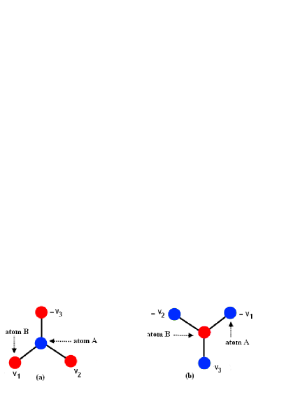
Figure 2:  (a) Nearest neighbors of a A- type atom. (b) Nearest neighbors of a B-type atom. These two configurations are precisely the representations $\mathbf{3}$  and $\mathbf{3}^{\ast}$ of $SU\left(3\right)$ .

This hidden $SU\left(3\right)$ invariance can be made more explicit by remarking that the relative vectors $\mathbf{v}_{1},$ $\mathbf{v}_{2},\mathbf{v}_{3}$ describing the three first closed neighbors to a $\mathcal{A}$- type carbon at site $\mathbf{r}_{i}$ of the honeycomb, together with their opposites $-\mathbf{v}_{n}$ for $\mathcal{B}$-type carbons, are precisely the weight vectors of the 3-dimensional representations of the $SU\left(3\right)$ symmetry, $\mathbf{v}_{n}=d\sqrt{\frac{3}{2}}\mathbf{\lambda}_{n}$. For readers not familiar with representation group theory terminology, we give here below as well in the beginning of section 3.a summary on the $SU\left(N\right)$ symmetry.

some useful tools on SU$\left(3\right)$
Roughly, the $SU\left(3\right)$ symmetry is the simplest extension of the $SU\left(2\right)$ symmetry group behind the spin of the electron. The basic relation $\mathbf{v}_{1}+\mathbf{v}_{2}+\mathbf{v}_{3}=\mathbf{0}$ of the honeycomb, which upon setting $\mathbf{v}_{n}=d\sqrt{\frac{3}{2}}\mathbf{\lambda}_{n}$, reads also as $\mathbf{\lambda}_{1}+\mathbf{\lambda}_{2}+\mathbf{\lambda}_{3}=\mathbf{0.}$ This constraint relation has an interpretation in $SU\left(3\right)$ representation theory; it should be put in one to one correspondence with the well known $SU\left(2\right)$ relation $(\frac{1}{2}-\frac{1}{2})=0$ of the spin $\frac{1}{2}$ representation;

$$\left(\begin{array}[]{c}\left|\frac{+1}{2}\right\rangle\\ \left|\frac{-1}{2}\right\rangle\end{array}\right)\equiv\underline{\mathbf{2}}$$

(2.4)

see also eq(3.3) for details. The basic properties of the $SU\left(3\right)$ symmetry are encoded in the so called Cartan matrix $K_{ij}$ and its inverse $K_{ij}^{-1}$ which read as

$$K_{ij}=\left(\begin{array}[]{cc}2&-1\\ -1&2\end{array}\right)$$ , .

(2.5)

These matrices can be also written as the intersection of 2D- vectors as $K_{ij}=\mathbf{\alpha}_{i}\cdot\mathbf{\alpha}_{j}$, $K_{ij}^{-1}=\mathbf{\omega}_{i}\cdot\mathbf{\omega}_{j}$ where $\mathbf{\alpha}_{1}$ and $\mathbf{\alpha}_{2}$ are the two simple roots of $SU\left(3\right)$ and where $\mathbf{\omega}_{1}$ and $\mathbf{\omega}_{2}$ are the corresponding two fundamental weights which related to the simple roots by the following duality relation

$$\mathbf{\alpha}_{i}\cdot\mathbf{\omega}_{j}=\delta_{ij}$$

(2.6)

Using these tools, the honeycomb relation $\mathbf{\lambda}_{1}+\mathbf{\lambda}_{2}+\mathbf{\lambda}_{3}=\mathbf{0}$ is naturally solved in terms of the fundamental weights as follows

$$\mathbf{\lambda}_{1}=\omega_{1},$$ .

(2.7)

We also have the following relations between the $\mathbf{a}_{i}$ vectors and the $\mathbf{v}_{i}$ ones: $\mathbf{a}_{1}=\left(\mathbf{v}_{1}-\mathbf{v}_{2}\right)$, $\mathbf{a}_{2}=\mathbf{v}_{2}-\mathbf{v}_{3}$ and $\mathbf{a}_{3}=\mathbf{v}_{3}-\mathbf{v}_{1}$. Notice that the vectors $\pm\mathbf{a}_{1},$ $\pm\mathbf{a}_{2},$ $\pm\mathbf{a}_{3}$ are, up to the scale factor $d\sqrt{\frac{3}{2}}$, precisely the six roots of the $SU\left(3\right)$ symmetry

$$\mathbf{a}_{1}=d\sqrt{\frac{3}{2}}\mathbf{\alpha}_{1},$$

(2.8)

where we have also used the remarkable relation between roots and weights that follow from eqs (2.5-2.6).

$$\mathbf{\alpha}_{1}=2\omega_{1}-\omega_{2},$$

(2.9)

2.2.2 Electronic properties

Quantum mechanically, there are two approaches to deal with the geometrical constraint relation (2.2). The first one is to work in real space and think about it as the conservation law of total space-time probability current densities at each site $\mathbf{r}_{i}$ of the honeycomb. The second approach relies on moving to the reciprocal space where this constraint relation and the induced electronic properties get a remarkable interpretation in terms of $SU\left(3\right)$ representations.

1) conservation of total current density
In the real space, the way we interpret eq(2.2) is in terms of the relation between the time variation of the probability density $\rho\left(t,\mathbf{r}_{i}\right)=\left|\phi\left(t,\mathbf{r}_{i}\right)\right|^{2}$ of the electron at site $\mathbf{r}_{i}$ and the sum $\sum_{n=1}^{3}\mathbf{J}_{\mathbf{v}_{n}}\left(t,\mathbf{r}_{i}\right)=\mathbf{J}\left(t,\mathbf{r}_{i}\right)$ of incoming and outgoing probability current densities along the $\mathbf{v}_{n}$- directions. On one hand, because of the equiprobability in hopping from the carbon at $\mathbf{r}_{i}$ to each one of the three nearest carbons at $\mathbf{r}_{i}+\mathbf{v}_{n}$, the norm of the $\mathbf{J}_{\mathbf{v}_{n}}$- vector current densities should be equal and so they should have the form

$$\mathbf{J}_{\mathbf{v}_{n}}\left(t,\mathbf{r}_{i}\right)=j\left(t,\mathbf{r}_{i}\right)\mathbf{e}_{n}$$ , .

(2.10)

These probability current densities together with the unit vectors $\mathbf{e}_{n}=\frac{\mathbf{v}_{n}}{d}$ pointing in the different $\mathbf{v}_{n}$- direction; but have the same non zero norm: $\left\|\mathbf{J}_{\mathbf{v}_{1}}\right\|=\left\|\mathbf{J}_{\mathbf{v}_{2}}\right\|=\left\|\mathbf{J}_{\mathbf{v}_{3}}\right\|=\left|j\right|$. Substituting in the above relation, the total probability current density $\mathbf{J}\left(t,\mathbf{r}_{i}\right)$ at the site $\mathbf{r}$ and time $t$ takes then the factorized form

$$\mathbf{J}\left(t,\mathbf{r}\right)=\frac{j\left(t,r\right)}{d}\left(\sum_{n}\mathbf{\lambda}_{n}\right).$$ (2.11)

On the other hand, by using the Schrodinger equation $i\hbar\frac{\partial\phi}{\partial t}=\left(-\frac{\hbar^{2}}{2m}\nabla^{2}+V\right)\phi$ describing the interacting dynamics of the electronic wave at $\mathbf{r}$, we have the usual conservation equation,

$$\frac{\partial\rho\left(t,\mathbf{r}\right)}{\partial t}+\mathop{\mathrm{d}iv}\mathbf{J}\left(t,\mathbf{r}\right)=0\text{ \ \ },$$ (2.12)

with probability density $\rho\left(t,\mathbf{r}\right)$ as before and $J=\frac{i\hbar}{2m}\left(\phi\nabla\phi^{\ast}-\phi^{\ast}\nabla\phi\right)$ with m the mass of the electron and $\phi=\phi\left(t,\mathbf{r}\right)$ its wave. Moreover, assuming $\frac{\partial\rho}{\partial t}=0$ corresponding to stationary electronic waves $\phi\left(t,\mathbf{r}\right)=e^{i\omega t}\phi\left(\mathbf{r}\right)$, it follows that the space divergence of the total current density vanishes identically; $\mathop{\mathrm{d}iv}\mathbf{J}=0$. This constraint equation shows that generally $\mathbf{J}$ should be a curl vector; but physical consideration indicates that we must have $\mathbf{J}\left(t,\mathbf{r}\right)=0$, in agreement with Gauss-Stokes theorem $\int_{\mathcal{V}}\mathop{\mathrm{d}iv}\mathbf{J}$ $d\mathcal{V}$ $\mathbf{=}$ $\int_{\partial\mathcal{V}}\mathbf{J.}d\mathbf{\sigma}$ leading to the same conclusion. Combining the property $\mathbf{J}\left(t,\mathbf{r}\right)=0$ with its factorized expression $\frac{j}{d}\left(\sum_{n}\mathbf{v}_{n}\right)$ given by eq(2.11) together with $j\neq 0$, we end with the constraint relation $\sum_{n}\mathbf{v}_{n}=0$.

2) conservation of total phase
In the dual space of the electronic wave of graphene, the constraint relation (2.2) may be interpreted in two different, but equivalent, ways; first in terms of the conservation of the total relative phase $\Delta\varphi_{{\scriptsize tot}}=\sum\mathbf{k.}\Delta\mathbf{r}$ of the electronic waves induced by the hopping to the nearest neighbors. The second way is in terms of the conservation of the total momenta at each site of the honeycomb.
Decomposing the wave function $\phi\left(\mathbf{r}\right)$, associated with a A-type carbon at site $\mathbf{r}$, in Fourier modes as $\sum_{\mathbf{k}}e^{i2\pi\mathbf{k}\cdot\mathbf{r}}$ $\tilde{\phi}\left(\mathbf{k}\right)$; and similarly for the B-type neighboring ones $\phi\left(\mathbf{r}+\mathbf{v}_{n}\right)=\sum_{\mathbf{k}}e^{i2\pi\mathbf{k}\cdot\mathbf{r}}$ $\tilde{\phi}_{n}\left(\mathbf{k}\right)$ with $\mathbf{k=}\left(k_{x},k_{y}\right)$, we see that $\tilde{\phi}\left(k\right)$ and the three $\tilde{\phi}_{n}\left(k\right)$ are related as

$$\tilde{\phi}_{n}\left(k\right)=e^{i2\pi\theta_{n}}\tilde{\phi}\left(k\right)$$ ,  ,

(2.13)

with relative phases $\theta_{n}=\mathbf{k}\cdot\mathbf{v}_{n}$. These electronic waves have the same module, $\left|\tilde{\phi}_{n}\left(k\right)\right|^{2}=\left|\tilde{\phi}\left(k\right)\right|^{2}$; but in general non zero phases; $\theta_{1}\neq\theta_{2}\neq\theta_{3}$. This means that in the hop of an electron with momentum $\mathbf{p}=\hbar\mathbf{k}$ from a site $\mathbf{r}_{i}$ to the nearest one at $\mathbf{r}_{i}+\mathbf{v}_{n}$, the electronic wave acquires an extra phase of an amount $\theta_{n}$; but the probability density at each site is invariant. Demanding the total relative phase to obey the natural condition,

$$\theta_{1}+\theta_{2}+\theta_{3}=0\text{ \ },\text{ \ \ }\mathop{\mathrm{m}od}\left(2\pi\right),$$ (2.14)

one ends with the constraint eq(2.2). Let us study two remarkable consequences of this special conservation law on the $\theta_{n}$ phases by help of the hidden $SU\left(3\right)$ symmetry of graphene. Using eq(2.7), which identifies the relatives $\mathbf{v}_{n}$ vectors with the weight vectors $\mathbf{\omega}_{n}$, as well as the duality relation $\mathbf{\alpha}_{i}\cdot\mathbf{\omega}_{j}=\delta_{ij}$ (2.6), we can invert the three equations $\theta_{n}=\mathbf{k}\cdot\mathbf{v}_{n}$ to get the momenta $\mathbf{p}_{n}\mathbf{=}\hbar\mathbf{k}_{n}$ of the electronic waves along the $\mathbf{v}_{n}$-directions. For the two first $\theta_{n}$’s, that is $n=1,2$, the inverted relations are nicely obtained by decomposing the 2D wave vector $\mathbf{k}$ along the $\mathbf{\alpha}_{1}$ and $\mathbf{\alpha}_{2}$ directions; that is $\mathbf{k}=k_{1}\mathbf{\alpha}_{1}+k_{2}\mathbf{\alpha}_{2}$; and end with the following particular solution,

$$\theta_{1}=k_{1}d,$$ .

(2.15)

2.3 Band structure

We first study the case of graphene monolayer; then we extend the result to the case of graphene bilayers by using the corresponding hidden symmetries.

2.3.1 Graphene monolayer

By considering a graphene sheet and restricting the tight binding hamiltonian (2.1) to the first nearest neighbor interactions namely,

$$H=-t\mathop{\displaystyle\sum}\limits_{\mathbf{r}_{i}}\sum_{n=1}^{2}a_{\mathbf{r}_{i}}b_{\mathbf{r}_{i}+\mathbf{v}_{n}}^{\dagger}+hc,$$ (2.16)

we can determine the energy dispersion relation and the delocalized electrons by using the $SU\left(3\right)$ symmetry of the 2D honeycomb. Indeed performing the Fourier transform of the various wave functions, we end with the following expression of the hamiltonian in the reciprocal space

$$H=$$ .

(2.17)

The diagonalization of this hamiltonian leads to the two eigenvalue $E_{\pm}=\pm t\left|\varepsilon_{\mathbf{k}}\right|$ giving the energy of the valence and conducting bands. In these relations, the complex number $\varepsilon_{\mathbf{k}}$ is an oscillating wave vector dependent function given by $\varepsilon_{\mathbf{k}}=e^{idQ_{1}}+e^{idQ_{2}}+e^{-id\left(Q_{1}+Q_{2}\right)}$ where we have set $Q_{l}=\mathbf{k}.\mathbf{\lambda}_{l}$. This relation, which is symmetric under permutation of the three $Q_{i}$, can be also rewritten by using the fundamental weights as follows,

$$\varepsilon_{\mathbf{k}}=\left(e^{id\left[\mathbf{k}.\mathbf{\omega}_{1}\right]}+e^{id\left[\mathbf{k}.\left(\mathbf{\omega}_{2}-\mathbf{\omega}_{1}\right)\right]}+e^{-id\left[\mathbf{k}.\mathbf{\omega}_{2}\right]}\right)$$ .

(2.18)

Up on expanding the wave vector as $\mathbf{k}=k_{1}\mathbf{\alpha}_{1}+k_{2}\mathbf{\alpha}_{2}$, this relation reads also as $\varepsilon_{\mathbf{k}}=e^{ik_{1}d}+e^{i\left(k_{2}-k_{1}\right)d}+e^{-ik_{2}d}$. Notice that from (2.18), we learn that $\varepsilon_{\mathbf{k}}$ is invariant under the translations $\mathbf{k}\rightarrow$ $\mathbf{k}+$ $\frac{2\pi}{d}\left(N_{1}\mathbf{\alpha}_{1}+N_{2}\mathbf{\alpha}_{2}\right)$ with $N_{1},$ $N_{2}$ arbitrary integers; thanks to the duality relation $\mathbf{\alpha}_{i}.\mathbf{\omega}_{j}=\delta_{ij}$.
Notice also that near the origin $\mathbf{k}=\mathbf{0}$, we have $\varepsilon_{\mathbf{k}}=3+O\left(\mathbf{k}^{2}\right)$, in agreement with non relativistic quantum mechanics. The three terms which are linear terms in $\mathbf{k}$ cancel each others due to the $SU\left(3\right)$ symmetry.

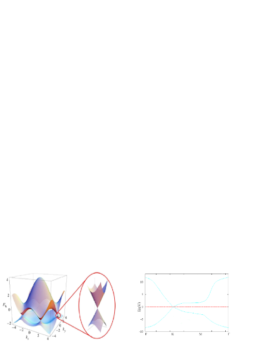
Figure 3: On left the band structure of the graphene monolayer where one recognizes the Dirac points. On right, it is shown the relativistic behavior near a Dirac point where conducting and valence bands touch.  On right the band structure in GGA approximation using QE  code.

Notice moreover that the Hamiltonian (2.16) has Dirac zeros located, up to lattice translations, at the following wave vectors

$$\left(k_{1},k_{2}\right)=\left\{\begin{array}[]{ccc}\frac{2\pi}{3d}\left(1,0\right)&,&-\frac{2\pi}{3d}\left(1,0\right)\\ \frac{2\pi}{3d}\left(0,1\right)&,&-\frac{2\pi}{3d}\left(0,1\right)\\ \frac{2\pi}{3d}\left(1,1\right)&,&-\frac{2\pi}{3d}\left(1,1\right)\end{array}\right.$$

(2.19)

Notice that these six zero modes, which read also as

$$\mathbf{K}_{1}^{\pm}=\pm\frac{2\pi}{3d}\left(2\mathbf{\omega}_{1}-\mathbf{\omega}_{2}\right),$$ ,

(2.20)

are not completely independent; some of them are related under lattice translations. For instance, the three $\mathbf{K}_{i}^{+}$ are related to each others as follows

$$\mathbf{K}_{1}^{+}+\frac{2\pi}{d}\mathbf{\omega}_{2}=\mathbf{K}_{2}^{+}+\frac{2\pi}{d}\mathbf{\omega}_{1}=\mathbf{K}_{3}^{+}$$ .

(2.21)

The same property is valid for the other three $\mathbf{K}_{i}^{-}$’s; so one is left with the usual $\mathbf{K}_{\pm}$ Dirac zeros of the first Brillouin zone,

$$\mathbf{K}_{\pm}=\pm\frac{2\pi}{3d}\left(\mathbf{\omega}_{1}+\mathbf{\omega}_{2}\right)=\pm\frac{2\pi}{3d}\left(\mathbf{\alpha}_{1}+\mathbf{\alpha}_{2}\right).$$ (2.22)

These two zeros are not related by lattice translations; but are related by a $\mathbb{Z}_{2}$ symmetry mapping the fundamental weights and the simple roots to their opposites.
We end this section by noting that the group theoretical approach developed in this study may be also used to deal with graphene multi-layers and cousin systems. Below, we describe briefly the bilayers; the cousin systems are studied in next sections.

2.3.2 Bilayer graphene

Bilayer graphene was studied for the first time in McCann & Falko, (2006). It was modeled as two coupled hexagonal lattices including inequivalent sites in the two different layers that are ranged in the Bernal stacking (the stacking fashion of graphite where the upper layer has its B sublattice on top of sublattice A of the underlying layer) as showed in the figure (4).

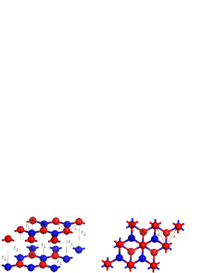
Figure 4: On right bilayer graphene in the AB stacking allotrope with hop energy t_⊥ between the layers. On right bilayer graphene projection in the x-y plane.

This leads to a break of the D_6h Bravais symmetry of the lattice with  respect to the c axis. Comparing bilayer graphene to monolayer one, we notice that its unit cell contains four atoms. There exist other arrangements such as the AA stacking, where the two lattices are directly above each other and bonds form between the same sublattices. The AB stacking arrangement was experimentally verified in epitaxial graphene by Ohta et al. (Ohta et al.,, 2007) . The tight-binding model describing bilayer graphene is an extension of the one corresponding to the monolayer (2.1), by adding interlayer hopping elements $H=H_{1}+H_{2}+H_{\bot}$ where H_i are as in (2.1) and where

$$H_{\bot}=$$ ,

(2.23)

with $t_{\bot}$ is the hop energy of the pi-electrons between layers calculated to be $t_{\bot}\sim\frac{t}{10}$ (Charlier et al.,, 1991). From the view of hidden symmetries, the bilayer graphene has a symmetry type $SU\left(3\right)\times SU\left(2\right)\times SU\left(3\right)$; each $SU\left(3\right)$ factor is associated with a graphene sheet; while the $SU\left(2\right)$ corresponds to the transitions between the two layers and is associated with propagation along the z-direction of the 3D-space.
Applying Fourier transform, the above hamiltonian can be rewritten in the following form:

$$H=$$ ,

(2.24)

with $\varepsilon_{\mathbf{k}}$ is as in eq(2.18). The diagonalization of this hamiltonian leads to the following energy dispersion relations,

$$E_{\mathbf{k}}^{\pm}=\pm\frac{1}{t}\sqrt{\left(t_{\bot}-t\varepsilon_{\mathbf{k}}^{\ast}\right)\left(t_{\bot}-t\varepsilon_{\mathbf{k}}\right)},$$ ,

(2.25)

The corresponding band structure has two additional bands, $\pi$ and $\pi^{\ast}$ states having lower energy bands, that is consequence of the number of atoms per unit cell. Neutral bilayer graphene is gapless McCann & Falko, (2006) and exhibits a variety of second-order effects.

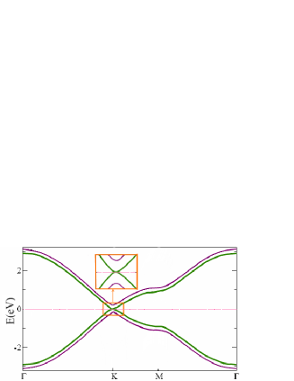
Figure 5: Band structure of the bilayer graphene

The studies on bilayer graphene show that it has many common physical properties with the monolayer, such as the exceptionally high electron mobility and high mechanical stability (Ohta et al.,, 2007)-Novoselov et al., (2006). The synthesis of bilayer graphene thin films was realized by deposition on a silicon carbide (SiC) substrate (Ohta et al.,, 2006). The measurements of their electronic band structure, using angle-resolved photo-emission spectroscopy (ARPES), suggest the control of the gap at the K Point by applying Coulomb potential between the two layers. This tuning of the band gap changed the biased bilayer from a conductor to a semiconductor.

3 Higher dimensional graphene systems

Motivated by the connection between 2D graphene and $SU\left(3\right)$ symmetry, we study in this section the extension of the physics of 2D graphene in diverse dimensions; that is 1D, 2D, 3D, 4D, and so on; the 2D case is obviously given by 2D graphene and its multi-layers considered in previous section. The precited dimensions are not all of them realizable in condensed matter physics; but their understanding may help to get more insight on the specific properties of 2D graphene since the $SU\left(3\right)$ is the second element of the $SU\left(N\right)$ symmetries series.
First we develop our proposal regarding higher dimensional graphene systems that are based on $SU\left(N\right)$ symmetry including the particular 1D poly-acetylene chain which corresponds to $SU\left(2\right)$ symmetry. Then, we compute the energy dispersion relation of these kinds of lattice quantum field theory (QFT). Explicit examples of such lattice fermionic models will be studied in the next sections.

3.1 The $SU\left(N\right)$ model

Higher dimensional graphene systems are abstract extensions of 2D graphene; the analogue of the 2D honeycomb is given by a real N-dimensional lattice $\mathcal{L}_{su\left(N\right)}$. The quantum hamiltonian describing these systems is a generalization of (2.1) and reads as follows,

$$H_{N}=$$

(3.1)

where $a_{\mathbf{r}_{i}}$, $b_{\mathbf{r}_{i}{\scriptsize+}\mathbf{v}_{n}}$, $a_{\mathbf{r}_{i}}^{\dagger}$, $b_{\mathbf{r}_{i}{\scriptsize+}\mathbf{v}_{n}}^{\dagger}$ are fermionic annihilation and creation operators living on $\mathcal{L}_{su\left(N\right)}$. Moreover the vectors $\mathbf{v}_{1},...,\mathbf{v}_{N}$ are, up to a global scale factor, the fundamental weights of the N-dimensional representation of the $SU\left(N\right)$ symmetry constrained by the typical property

$$\mathbf{v}_{1}+...+\mathbf{v}_{N}=0.$$ (3.2)

The vectors $\mathbf{V}_{nm}=\left(\mathbf{v}_{n}-\mathbf{v}_{m}\right)$ are, up to a scale factor, precisely the $N\left(N-1\right)$ roots of $SU\left(N\right)$; they obey as well the group property $\sum\mathbf{V}_{nm}=0$.
These particular features of $H_{N}$ let understand that its physical properties are expected to be completely encoded by the hidden $SU\left(N\right)$ symmetry of the model. Below, we show that this is indeed the case; but for simplicity we will focus on the first term of $H_{N}$; i.e working in the limit $t^{\prime}\rightarrow 0$.

3.1.1 Useful tools on $SU\left(N\right)$ symmetry

Since one of our objectives in this paper is to use the $SU\left(N\right)$ symmetry of the crystals to study higher dimensional graphene systems; and seen that readers might not be familiar with these tools; we propose to give in this subsection some basic tools on $SU\left(N\right)$ by using explicit examples.

a) cases $SU\left(2\right)$ and $SU\left(3\right)$
The $SU\left(2\right)$ symmetry is very familiar in quantum mechanics; it is the symmetry that describes the spin of the electrons and the quantum angular momentum states.
Roughly speaking, the $SU\left(2\right)$ symmetry is a 3-dimensional space generated by three matrices which can be thought of as the usual traceless Pauli matrices

$$\sigma^{0}=\left(\begin{array}[]{cc}\frac{1}{2}&0\\ 0&-\frac{1}{2}\end{array}\right),$$ ,

(3.3)

involving one diagonal matrix $\sigma^{0},$ giving the charge operator, and two nilpotent matrices $\sigma^{\pm}$ interpreted as the step operators or equivalently the creation and annihilation operators in the language of quantum mechanics. These three matrices obey commutation relations $\left[\sigma^{0},\sigma^{\pm}\right]=\pm 2\sigma^{\pm}$ that define the $su\left(2\right)$ algebra. Observe also the traceless property of the charge operator $Tr\sigma^{0}=\frac{1}{2}-\frac{1}{2}=0$, which should be related to the constraint relation (3.2) with $N=2$.
The $SU\left(3\right)$ symmetry group is 8-dimensional space generated by 8 matrices which can be denoted as

$$h_{1},h_{2},$$ ,

(3.4)

with $h_{1},$ $h_{2}$ two diagonal matrices defining the charge operators and six step operators $e^{\pm\alpha_{1}},$ $e^{\pm\alpha_{2}},$ $e^{\pm\alpha_{3}}$ playing the role of creation and annihilation operators. The $e^{\pm\alpha_{i}}$’s are nilpotent and are related as $\left(e^{-\alpha_{i}}\right)^{+}=e^{+\alpha_{i}}$. An example of these matrices is given by the following $3\times 3$ matrices

$$\ \ \ \ \ \ \ \ \ \ \ {\small h}_{1}{\small=}\left(\begin{array}[]{ccc}{\small\mu}_{1}&{\small 0}&{\small 0}\\ {\small 0}&{\small\mu}_{2}&{\small 0}\\ {\small 0}&{\small 0}&{\small\mu}_{3}\end{array}\right),$$

(3.5)

with the traceless property of the charge operators which reads as follows

$$\mathbf{\lambda}_{1}+\mathbf{\lambda}_{2}+\mathbf{\lambda}_{3}=0$$ , ,

(3.6)

and which should be compared with the case $N=3$ in (3.2).
The vectors $\mathbf{\alpha}_{1}$ and $\mathbf{\alpha}_{2}$ are the simple roots encountered in the previous section; their scalar product $\mathbf{\alpha}_{i}.\mathbf{\alpha}_{j}$ gives precisely the Cartan matrix $\mathbf{K}_{ij}$ of eq(2.5).

b) case $SU\left(N\right)$
In the general case $N\geq 2$, the corresponding $SU\left(N\right)$ symmetry is $\left(N^{2}-1\right)$-dimensional space generated by $\left(N^{2}-1\right)$ matrices; $N-1$ of them are diagonal

$$h_{1},$$

(3.7)

and are interpreted as the charge operators; and $N\left(N-1\right)$ step operators giving the creation and annihilation operators $e^{+\alpha},$ $e^{-\alpha}$ with $\mathbf{\alpha}$ standing for generic roots containing the two following:
(a) N-1 simple ones namely $\mathbf{\alpha}_{1}\mathbf{,\alpha}_{2}\mathbf{,...,\alpha}_{N-1}$ (together with their opposites) whose scalar products $\mathbf{\alpha}_{i}.\mathbf{\alpha}_{j}$ give precisely the following $\left(N-1\right)\times\left(N-1\right)$ Cartan matrix

$$\mathbf{K}=\left(\begin{array}[]{cccccc}2&-1&0&\cdots&0&0\\ -1&2&-1&&0&0\\ 0&-1&2&&0&0\\ \vdots&&&\ddots&&\vdots\\ 0&0&0&&2&-1\\ 0&0&0&\cdots&-1&2\end{array}\right),$$ (3.8)

(b) non simple roots given by linear (positive and negative) combinations of the simple ones; these roots are given by $\pm\mathbf{\beta}_{ij}=\pm\left(\mathbf{\alpha}_{i}+...+\mathbf{\alpha}_{j}\right)$ with $1\leq i<j\leq N-1.$
Notice that the above Cartan matrix $\mathbf{K}$ and its inverse

$$\mathbf{K}^{-1}=\left(\begin{array}[]{cccccc}\frac{N}{N+1}&\frac{N-1}{N+1}&\frac{N-2}{N+1}&\cdots&\frac{2}{N+1}&\frac{1}{N+1}\\ \frac{N-1}{N+1}&\frac{2\left(N-1\right)}{N+1}&\frac{2\left(N-2\right)}{N+1}&\cdots&\frac{4}{N+1}&\frac{2}{N+1}\\ \frac{N-2}{N+1}&\frac{2\left(N-2\right)}{N+1}&\frac{3\left(N-2\right)}{N+1}&\cdots&\frac{6}{N+1}&\frac{3}{N+1}\\ \vdots&\vdots&\vdots&\ddots&\vdots&\vdots\\ \frac{2}{N+1}&\frac{4}{N+1}&\frac{6}{N+1}&\cdots&\frac{2\left(N-1\right)}{N+1}&\frac{N-1}{N+1}\\ \frac{1}{N+1}&\frac{2}{N+1}&\frac{3}{N+1}&\cdots&\frac{N-1}{N+1}&\frac{N}{N+1}\end{array}\right)$$ (3.9)

capture many data on the $SU\left(N\right)$ symmetry; they give in particular the expression of the simple roots $\mathbf{\alpha}_{1}\mathbf{,\alpha}_{2}\mathbf{,...,\alpha}_{N-1}$ in terms of the fundamental weights $\mathbf{\omega}_{1},...,\mathbf{\omega}_{N-1}$ and vice versa; that is $\mathbf{\alpha}_{i}=\sum_{j}K_{ij}\mathbf{\omega}_{j}$ and $\mathbf{\omega}_{i}=\sum_{j}K_{ij}^{-1}\mathbf{\alpha}_{j}$. Recall that simple roots and fundamental weights obey the duality property $\mathbf{\alpha}_{i}.\mathbf{\omega}_{j}=\delta_{ij}$; we also have $\mathbf{\omega}_{i}.\mathbf{\omega}_{j}=K_{ij}^{-1}$.

3.1.2 The lattice $\mathcal{L}_{su\left(N\right)}$

The lattice $\mathcal{L}_{su\left(N\right)}$ is a real $\left(N-1\right)$- dimensional crystal with two superposed integral sublattices $\mathcal{A}_{N}$ and $\mathcal{B}_{{}_{N}}$; each site $\mathbf{r}_{\mathbf{m}}$ of these sublattices is generated by the $SU\left(N\right)$ simple roots $\mathbf{\alpha}_{1},...,\mathbf{\alpha}_{N-1}$;

$$\mathbf{r}_{\mathbf{m}}$$ ,

(3.10)

with $m_{i}$ integers; for illustration see the schema (a), (b), (c) of the figure (6) corresponding respectively to $N=2,3,4$; and which may be put in one to one with the $sp^{1}$, $sp^{2}$ and $sp^{3}$ hybridization of the carbon atom orbital $2s$ and $2p$.

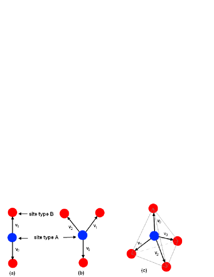
Figure 6: (a) 1A+2B lattice sites of $\mathcal{L}_{su\left(2\right)}$; A-type in blue and B-type in red; the 2B form a $su\left(2\right)$  doublet. (b) 1A+3B sites of $\mathcal{L}_{su\left(3\right)}$;  the 3B form a $su\left(3\right)$ triplet. (c) 1A+4B sites of $\mathcal{L}_{su\left(4\right)}$ with 4B sites forming a regular tetrahedron.

On each lattice site $\mathbf{r}_{m}$ of $\mathcal{L}_{su\left(N\right)}$; say of A-type, lives a quantum state $A_{\mathbf{r}_{m}}$ coupled to the nearest neighbor states; in particular the first nearest states $B_{\mathbf{r}_{m}+\mathbf{v}_{i}}$ and the second nearest ones $A_{\mathbf{r}_{m}+\mathbf{V}_{ij}}$.
Generally, generic sites in $\mathcal{L}_{su\left(N\right)}$ have the following properties:
(1) $N$ first nearest neighbors with relative position vectors $\mathbf{v}_{i}$ constrained as

$$\mathbf{v}_{1}+\ldots+$$ .

(3.11)

These constraint relations are solved in terms of the $SU\left(N\right)$ weight vectors $\mathbf{\lambda}_{i}$ (resp. $-\mathbf{\lambda}_{i}$) of the fundamental (anti-fundamental) representation as follows

$$\mathbf{v}_{i}$$ ,

(3.12)

where $d$ is the relative distance between the closest $\mathcal{L}_{su\left(N\right)}$ sites. The $\mathbf{\lambda}_{i}$’s which satisfy $\mathbf{\lambda}_{1}+\ldots+$ $\mathbf{\lambda}_{N}=0$ can be nicely expressed in terms of the fundamental weights $\mathbf{\omega}_{1},...,\mathbf{\omega}_{N-1}$ as follows

$$\mathbf{\lambda}_{1}=\mathbf{\omega}_{1},$$ .

(3.13)

From the QFT view, this means that the quantum states at $\mathbf{r}_{m}+\mathbf{v}_{i}$ sites are labeled by the $\mathbf{\lambda}_{i}$ weights as $B_{\mathbf{r}_{m}+\mathbf{v}_{i}}\equiv B_{\mathbf{\lambda}_{i}}\left(\mathbf{r}_{m}\right)$ and so the multiplet

$$\left(\begin{array}[]{c}|\mathbf{\lambda}_{1}>\\ \vdots\\ |\mathbf{\lambda}_{N}>\end{array}\right)\equiv$$  ,

(3.14)

transform in the fundamental representation of $SU\left(N\right)$.
(2) $N\left(N-1\right)$ second nearest neighbors of A-type with relative position vectors $\mathbf{V}_{ij}$ given by $\mathbf{v}_{i}-\mathbf{v}_{j}$ and obeying the constraint relation $\sum_{i,j}\mathbf{V}_{ij}=0.$ This condition is naturally solved by (3.11) and (3.12) showing that the relative vectors between second nearest neighbors are proportional to $SU\left(N\right)$ roots $\mathbf{\beta}_{ij}$ like

$$\mathbf{V}_{ij}=a\mathbf{\beta}_{ij}$$ ,

(3.15)

and so the condition $\sum\mathbf{V}_{ij}=0$ turns to a $SU\left(N\right)$ property on its adjoint representation labeled by the roots.

3.2 Energy dispersion relation

Restricting the analysis to the first nearest neighbors described by eq(3.1) in the limit $t^{\prime}\rightarrow 0$, the hamiltonian $H_{N}$ on $\mathcal{L}_{su\left(N\right)}$ reduces to

$$H_{N}=$$ ,

(3.16)

where now $\mathbf{r}_{i}$ and $\mathbf{v}_{n}$ are $\left(N-1\right)$- dimensional vectors. By using the Fourier transform of the field operators $a_{\mathbf{r}_{i}}$ and $B_{\mathbf{r}_{m}+\mathbf{v}_{i}}^{\pm}$ namely,

$$a_{\mathbf{r}_{i}}\sim\mathop{\displaystyle\sum}\limits_{\mathbf{k}}e^{i\mathbf{k.r}_{m}}a_{\mathbf{k}}^{\pm}$$ ,

(3.17)

we can put the hamiltonian $H_{N}$ as a sum over the wave vectors $\mathbf{k}$ in the following way;

$$H_{N}=\mathop{\displaystyle\sum}\limits_{\mathbf{k}}\left(a_{\mathbf{k}}^{\dagger},b_{\mathbf{k}}^{\dagger}\right)\left(\begin{array}[]{cc}0&\varepsilon_{\mathbf{k}}\\ \varepsilon_{\mathbf{k}}^{\ast}&0\end{array}\right)\left(\begin{array}[]{c}a_{\mathbf{k}}\\ b_{\mathbf{k}}\end{array}\right)$$ ,

(3.18)

with $\varepsilon_{\mathbf{k}}=t\sum_{i}e^{ia\mathbf{k}.\mathbf{\lambda}_{i}}$. This complex number can be also written as $t\sum_{i}e^{ia\mathbf{k}.\left(\mathbf{\omega}_{i}-\omega_{i-1}\right)}$ with $\omega_{-1}=0=\omega_{N}$. The energy dispersion relation of the "valence" and "conducting" bands are obtained by diagonalizing the hamiltonian $H_{N}$; they are given by $\pm\left|\varepsilon_{\mathbf{k}}\right|$ with,

$$\left|\varepsilon_{\mathbf{k}}\right|=t\sqrt{N+2\mathop{\displaystyle\sum}\limits_{i<j=1}^{N}\cos\left[a\mathbf{k}.\left(\mathbf{\lambda}_{i}\mathbf{-\lambda}_{j}\right)\right]}$$ .

(3.19)

Notice that $\left|\varepsilon_{\mathbf{k}}\right|$ depends remarkably in the difference of the weights $\mathbf{\lambda}_{i}\mathbf{-\lambda}_{j}$; which by help of eq(3.13), can be completely expressed in terms of the fundamental weights.
To get the Fermi wave vectors $\mathbf{k}_{F}$ for which the oscillating multi-variable function $\varepsilon_{\mathbf{k}}=t\sum_{l}e^{ia\mathbf{k}.\mathbf{\lambda}_{l}}$ vanish, we will proceed as follows: First, we work out an explicit example; then we give the general result. To that purpose, we expand the wave vector $\mathbf{k}$ in the weight vector basis as follows,

$$\mathbf{k}=\mathop{\displaystyle\sum}\limits_{i=1}^{N-1}Q_{i}\mathbf{\omega}_{i},$$ ,

(3.20)

and focus on working out the solution for the particular case where all the $Q_{i}$’s are equal, i.e: $Q_{1}=Q_{2}=...=Q_{N-1}=Q.$ General solutions are obtained from this particular case by performing lattice translations along the $\mathbf{\omega}_{i}$-directions; this leads to the new values $Q_{l}=Q+\frac{2\pi n_{l}}{N}$ with $n_{l}$ integers. Obviously, one may also expand the wave vector $\mathbf{k}$ like

$$\mathbf{k=}\mathop{\displaystyle\sum}\limits_{i=1}^{N-1}k_{i}\mathbf{\alpha}_{i}$$ , .

(3.21)

But this is equivalent to (3.20); the relation between the $Q_{l}$’s and the $k_{l}$’s is obtained by substituting $\mathbf{\alpha}_{i}=\sum_{j}K_{ij}\mathbf{\omega}_{j}$ into (3.21) and identifying it with (3.20). To compute the factors $e^{ia\mathbf{k}.\mathbf{\lambda}_{l}}$, we express the vectors $\mathbf{\lambda}_{l}$ in terms of the simple roots as follows

$$\mathbf{\lambda}_{1}=\mathbf{\omega}_{1},$$

(3.22)

then we use the root/weight duality relation $\mathbf{\omega}_{i}.\mathbf{\alpha}_{j}=\delta_{ij}$ as well as the simple choice $Q_{l}=Q$ to put the scalar product $\mathbf{k}.\mathbf{\lambda}_{l}$ into the following form $\left(\mathbf{k}.\mathbf{\lambda}_{l}\right)=\left(\mathbf{k}.\mathbf{\omega}_{1}\right)-lQ$, $l=1,...,N-1.$  Putting this expression back into $\varepsilon_{\mathbf{k}}$ and setting $\xi=e^{iaQ}$, we obtain $\varepsilon_{\mathbf{k}}=e^{ia\mathbf{k}.\mathbf{\omega}_{1}}\left[1+\xi+...+\xi^{N-1}\right]=0$ which is exactly solved by the N-th roots of unity namely

$$Q=\pm\frac{2s\pi}{aN}$$ , .

(3.23)

Therefore the Dirac points are, up to lattice translations, located at the wave vectors $\mathbf{k}_{s}=\pm\frac{2s\pi}{aN}\sum_{i}\mathbf{\omega}_{i}=\pm\frac{2s\pi}{aN}\sum_{i}\mathbf{\alpha}_{i}.$

4 Leading models

In this section, we study the cases $N=2,4$ as $N=3$ corresponds precisely to the 2D graphene before. The case $N=5$ will be studied in the next section seen its remarkable relation with 4D lattice QCD.

4.1 The $su\left(2\right)$ model

In this case, the lattice $\mathcal{L}_{su\left(2\right)}$, which is depicted in the figure (7), is a one dimensional chain with coordinate positions $\mathbf{r}_{m}=ma$ where $a$ is the site spacing and $m$ an arbitrary integer.

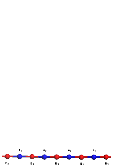
Figure 7: the lattice $\mathcal{L}_{su\left(2\right)}$  given by the superposition of two sublattices $\mathcal{A}_{su\left(2\right)}$  (in blue) and $\mathcal{B}_{su\left(2\right)}$ (in red). The atoms may be thought of as carbons in the ${sp}^{{1}}$  hybridization state.

Examples of carbon chains with delocalized electrons are given by one of the three following molecules

      chain               molecule delocalized electrons

polyacetylene $${\small...-CH=CH-CH=CH-CH-...}$$          1

cumulene          2

poly-yne          2

(4.1)

These molecules can be taken as the graphene bridge ultimately narrowed down to a few- carbon atoms or a single-atom width (Giritet et al.,, 2009; Koskinen et al.,, 2008; Jun,, 2008). Each site of $\mathcal{L}_{su\left(2\right)}$ has two first nearest neighbors forming an $su\left(2\right)$ doublet; and two second nearest ones that are associated with the two roots $\pm\alpha$ of $su\left(2\right)$ in agreement with the generic result summarized in the table,

nearest neighbors $$SU\left(N\right)$$

           first

           second

(4.2)

In the $SU\left(2\right)$ lattice model, eqs(3.2) read as

$$\mathbf{v}_{0}+\mathbf{v}_{1}=0$$ , (a)

, (b)

(4.3)

and are solved by the fundamental weights $\lambda_{1}=+\frac{1}{2},$ $\lambda_{2}=-\frac{1}{2}$ of the $SU\left(2\right)$ fundamental representation; i.e the isodoublet.

1) polyacetylene
The hamiltonian of the polyacetylene, where each carbon has one delocalized electron, is given by

$$H_{t}$$ .

(4.4)

Substituting $N=2$ in (3.19), we get the following energy dispersion relation

$$\left|\varepsilon_{k}\right|=t\sqrt{2+2\cos\left(2ak\right)}$$ (4.5)

which is also equal to $2t\cos\left(ka\right)$ in agreement with the expression $\varepsilon_{k}=t\left(e^{iak}+e^{-iak}\right)$; see also figure (8). Moreover, the vanishing condition $\varepsilon_{2}\left(k\right)=0$ is solved by the wave vectors $k_{\pm}=\pm\frac{\pi}{2a}$ $\mathop{\mathrm{m}od}\left(\frac{2\pi}{a}\right)$.

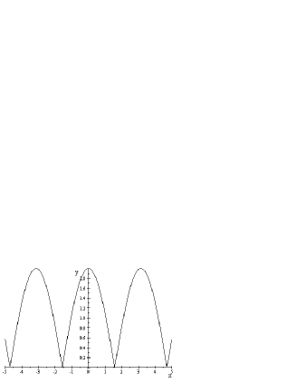
Figure 8: Energy dispersion relation of 1D poly-acetylene chain.

2) cumulene and poly-yne
In the case of cumulene and poly-yne, the two delocalized electrons are described by two wave functions $\phi_{{}_{\mathbf{r}_{m}}}^{1}$, $\phi_{{}_{\mathbf{r}_{m}}}^{2}$. The tight binding hamiltonian modeling the hopping of these electrons is a generalization of $H_{t}$. Let $a_{\mathbf{r}_{m}}^{\alpha}$, $a_{\mathbf{r}_{m}}^{\alpha+}$, $\alpha=1,2$ (resp. $b_{\mathbf{r}_{m}\pm a}^{\alpha}$, $b_{\mathbf{r}_{m}\pm a}^{\alpha+}$) be the annihilation and creation operators at the site $\mathbf{r}_{m}$ (resp. $\mathbf{r}_{m}\pm a$), the hamiltonian reads as follows

$$H_{t,t^{\prime}}$$ ,

(4.6)

where $t_{\alpha\beta}$ and $t_{\alpha\beta}^{\prime}$ are hop energy matrices which are identical for cumulene ($t_{\alpha\beta}=t_{\alpha\beta}^{\prime}$), but different for poly-yne ($t_{\alpha\beta}\neq t_{\alpha\beta}^{\prime}$). Mapping this hamiltonian to the reciprocal space, we get

$$H_{t,t^{\prime}}$$ ,

(4.7)

with

$$A\left(k\right)=$$

(4.8)

Now, using the fact that the two delocalized electrons are indistinguishable, it is natural to assume the following relations on the hop energies $t_{11}=t_{22}$, $t_{12}=t_{21}$ and the same thing for the $t_{\alpha\beta}^{\prime}$ matrix. This leads to the relations $A=D$, $B=C$ and so the above hamiltonian simplifies. In this case, the four energy eigenvalues are given by

$$E_{\pm}=$$ ,

,

(4.9)

and the zeros modes are given by $e^{2ika}=-\frac{t_{11}^{\prime}}{t_{11}}=-\frac{t_{12}^{\prime}}{t_{12}}$. Since in the case of cumulene we have $t_{\alpha\beta}=t_{\alpha\beta}^{\prime}$,  it follows that the zero modes are located as $k=\pm\frac{\pi}{2a}$ $\mathop{\mathrm{m}od}\frac{2\pi}{a}$.

3) nanoruban
We end this paragraph noting that such analysis may be also extended to the particular case of the periodic chain made by the junction of hexagonal cycles as depicted in the figure (9).

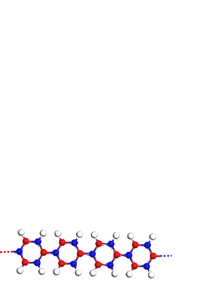
Figure 9: a periodic chain in 3D space with unit cells given by hexagonal cycles. Each cycle has six delocalized electrons.

This chain, which can be also interpreted as the smallest graphene nanoruban, is very particular from several issues; first its unit cells can be taken as given by the hexagonal cycles; second amongst the 6 carbons of the unit cycle, 4 of them have two first nearest neighbors and the 2 others have three first nearest ones. The third particularity is that the tight binding description of this chain is somehow more complicated with respect to the previous examples. Below we focus on the electronic properties of a given cycle by using the same approach we have been considering in this study.

4.2 Kekulé cycles

Kekulé cycles are organic molecules named in honor to the German chemist Friedrich Kekulé known for his works on tetravalent structure of carbon and the cyclic structure of benzene $C_{6}H_{6}$. These molecules; in particular the family $C_{n}H_{n}$ with $n\geq 3$, may be thought of as one dimensional cycles living in the 3D space; they involve carbon atoms (eventually other atoms such as Nitrogen) arranged in a cyclic lattice with both $\sigma$- and $\pi$-bonds. All these carbon atoms are in the sp² hybridization; they have 3n  covalent $\sigma$-bonds defining a quasi-planar skeleton; and n delocalized $\pi$-bonds with Pi electron orbital expanding in the normal direction as shown in the examples of fig(10).

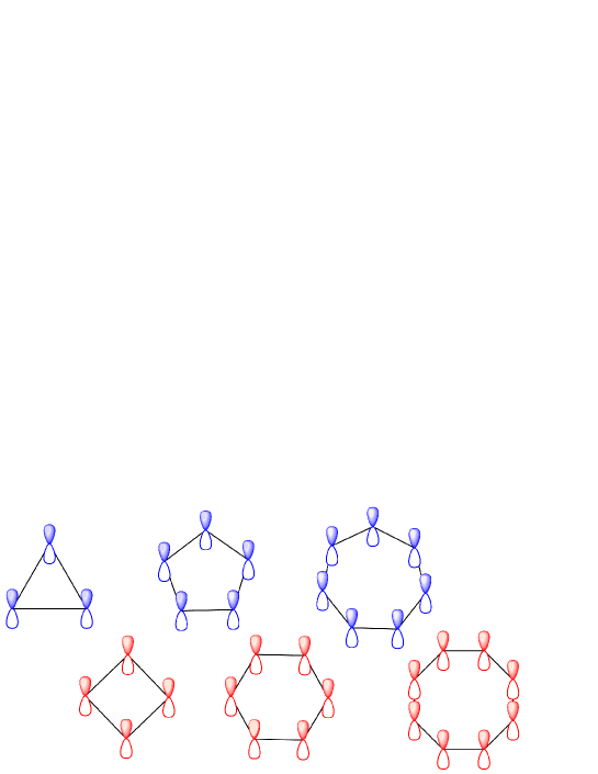
Figure 10: Six examples of Kekulé cycles type C_n H_n  with $n=3,4,5,6,7,8$ . The cations C⁺  of these molecules form a heavy skeleton represented by n-polygons. The orbitals in the normal direction are associated with the delocalized Pi-electrons.

Our interest into Kekulé molecules, in particular to the $C_{2N}H_{2N}$ family, comes from the fact that they can be viewed as the 1D analogue of the 2D graphene monolayer; they may be also obtained from the poly-acetylene chain by gluing the ends. It is then interesting to explore the electronic properties of this special class of systems by using the tight binding model and symmetries. To illustrate the method, we focus on the benzene $C_{6}H_{6}$ thought of as the superposition of two $C_{3}H_{3}$ sub-molecules as depicted in figure (11).

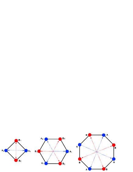
Figure 11: Kekulé molecules as the superposition of two sublattices. Sublattice $A$  in blue and sublattice $\mathcal{B}$ in red. Except the benzene, these molecules are generally are non planar.

From group theory view, the positions $\mathbf{v}_{1},$ $\mathbf{v}_{2},$ $\mathbf{v}_{3},$ $\mathbf{v}_{4},$ $\mathbf{v}_{5},$ $\mathbf{v}_{6}$ of the carbon atoms are given by the six roots of the $SU\left(3\right)$ symmetry.; that is

$$\mathbf{v}_{i}=a\mathbf{\alpha}_{i}$$ , ,

(4.10)

where $a=1.39$ $\mathring{A}$ and where the three $\mathbf{\alpha}_{i}$’s are as in section 2.

tight binding description
The electronic properties of the $C_{6}H_{6}$ are captured by the pi-electrons of the carbons. Denoting by $\mathbf{a}_{\mathbf{\mathbf{r}_{i}}}^{\dagger}$, $\mathbf{a}_{\mathbf{\mathbf{r}_{i}}}$ (resp. $\mathbf{b}_{\mathbf{\mathbf{r}_{i}}}^{\dagger}$, $\mathbf{b}_{\mathbf{\mathbf{r}_{i}}}$) the usual electronic creation and annihilation operators associated with the A_i (B_j) atoms in the sublattice $\mathcal{A}_{benz}$ ($\mathcal{B}_{benz}$), the tight binding hamiltonian of the benzene, restricted to first nearest neighbors, reads as follows,

$$H_{benz}=$$ .

(4.11)

In this relation, the position vectors $\mathbf{r}_{lm}$ have two indices; $l$ and $m$. The first one takes the values $l=1,2,3$; it indexes the three atoms in $\mathcal{A}_{benz}$; and the three ones in $\mathcal{B}_{benz}$. These positions are as follows,

$$\mathbf{r}_{2l-1,m}^{A}=\mathbf{r}_{1m}^{A},$$ , .

(4.12)

The second integer is an arbitrary number ($m\in\mathbb{Z}$); it captures the periodicity of the cycle and encodes in some sense the rotational invariance with respect to the axis of the planar molecule.
To fix the ideas, think about $\mathbf{r}_{lm}$ as the l-th electron in the sublattice $\mathcal{A}_{benz}$; that is $\mathbf{r}_{lm}\equiv\mathbf{r}_{2l-1,m}^{A}$. After a hop of this electron to the two first nearest carbons in $\mathcal{B}_{benz}$, the new position is

$$\mathbf{r}_{2l,m}^{B}=\mathbf{r}_{lm}+\mathbf{v}_{lj}$$ , .

(4.13)

where the $\mathbf{v}_{lj}$s are the relative positions of the first nearest neighbors.
Taking the Fourier transform of the creation and annihilation operators, $c_{\mathbf{r}_{n}}^{\pm}=\sum_{k}e^{\pm i\mathbf{k.r}_{n}}c_{\mathbf{k}}^{\pm}$ with $c_{\mathbf{k}}^{\pm}$ standing for $a_{\mathbf{k}}^{\pm}$, $b_{\mathbf{k}}^{\pm}$, we get an expression involving the product of three sums $\sum_{\mathbf{k}}$ $\sum_{\mathbf{k}^{\prime}}$ $\sum_{m}$. Then, using the discrete rotational invariance with respect to the axis of the molecule, we can eliminate the sum $\sum_{m}$ in terms of a Dirac delta function $\delta_{2}\left(\mathbf{k}-\mathbf{k}^{\prime}\right)$ and end, after integration with respect $\mathbf{k}^{\prime}$, with the following result,

$$\mathcal{H}_{benz}=\sum\limits_{\mathbf{k}}\text{ }\left(a_{\mathbf{k}},b_{\mathbf{k}}\right)\left(\begin{array}[]{cc}0&\varepsilon_{\mathbf{k}}\\ \varepsilon_{\mathbf{k}}^{\ast}&0\end{array}\right)\left(\begin{array}[]{c}a_{\mathbf{k}}^{\dagger}\\ b_{\mathbf{k}}^{\dagger}\end{array}\right)$$ .

(4.14)

with

$$\varepsilon_{\mathbf{k}}=-t\sum\limits_{l=1}^{3}\left(e^{i\mathbf{k}.\mathbf{v}_{l-}}+e^{i\mathbf{k}.\mathbf{v}_{l+}}\right)$$ .

(4.15)

Notice that like in graphene, the above hamiltonian has two eigenvalues $\pm\left|\varepsilon_{\mathbf{k}}\right|$. Moreover, substituting the $\mathbf{v}_{l\pm}$’s by their explicit expressions in terms of the $SU\left(3\right)$ roots $\mathbf{\alpha}_{l}$, we obtain the following dispersion relation together with a constraint relation capturing the planarity property of the molecule

$$\varepsilon_{\mathbf{k}}=-2t\sum\limits_{l=0}^{2}\cos\left(\frac{a\sqrt{2}}{2}\mathbf{k}.\mathbf{\alpha}_{l}\right),$$ .

(4.16)

Notice that the constraint equation $\eta_{\mathbf{k}}=0$ allows us to express the $k_{2}$ component of the wave vector in terms of $k_{1}$ and vice versa as depicted in fig(12). This relation plays a crucial role in the determination of the wave vectors at the Fermi level.

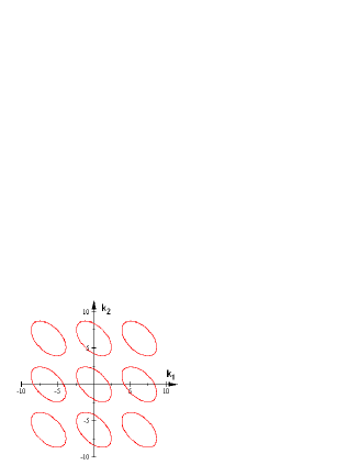
Figure 12: the plot of the energy dispersion relation $\varepsilon_{k_{1},k_{2}}$  and the constraint relation $\eta_{k_{1},k_{2}}$  $=$  $\sin k_{1}$  $+\sin k_{2}$  $-\sin\left(k_{1}+k_{2}\right)$  $=0$  in the reciprocal space.

4.3 The diamond model

The diamond model lives on the lattice $\mathcal{L}_{su\left(4\right)}$; this is a 3-dimensional crystal given by the superposition of two isomorphic sublattices $\mathcal{A}_{4}$ and $\mathcal{B}_{4}$ along the same logic as in the case of the 2D honeycomb. Each site $\mathbf{r}_{m}$ in $\mathcal{L}_{su\left(4\right)}$ has 4 first nearest neighbors at $\left(\mathbf{r}_{m}+\mathbf{v}_{i}\right)$ forming the vertices of a regular tetrahedron. A way to parameterize the relative positions $\mathbf{v}_{i}$ with respect to the central position at $\mathbf{r}_{m}$ is to embed the tetrahedron inside a cube; in this case we have:

$$\mathbf{v}_{1}=\frac{d}{\sqrt{3}}\left(-1,-1,+1\right)$$ ,

,

(4.17)

Clearly these vectors satisfy the constraint relation $\mathbf{v}_{0}+\mathbf{v}_{1}+\mathbf{v}_{2}+\mathbf{v}_{3}=0$. Having these expressions, we can also build the explicit positions of the 12 second nearest neighbors; these are given by $\mathbf{V}_{ij}=\mathbf{v}_{i}-\mathbf{v}_{j}$; but are completely generated by the following basis vectors

$$\mathbf{R}_{1}=\frac{d}{\sqrt{3}}\left(2,2,0\right)$$ , ,

(4.18)

that are related to $\mathbf{V}_{ij}$ as $\mathbf{R}_{i}=\mathbf{V}_{\left(i-1\right)i}$. We also have:

• the intersection matrix of the $\mathbf{R}_{i}$ vectors

  $$\mathbf{R}_{i}.\mathbf{R}_{j}=\frac{4d^{2}}{3}\mathbf{K}_{ij}$$ (4.19)

  with

  $$\mathbf{K}_{ij}=\left(\begin{array}[]{ccc}2&-1&0\\ -1&2&-1\\ 0&-1&2\end{array}\right)$$ ,

  (4.20)

• the special relation linking the $\mathbf{R}_{i}$’s and $\mathbf{v}_{0}$,

  $$\frac{3}{4}\mathbf{R}_{1}+\frac{2}{4}\mathbf{R}_{2}+\frac{1}{4}\mathbf{R}_{3}=\mathbf{v}_{0}$$ .

  (4.21)

Concerning the vector positions of the remaining 9 second neighbors, 3 of them are given by $-R_{1},-R_{2},-R_{3}$ and the other 6 by the linear combinations $R_{4}=V_{02},$ $R_{5}=V_{13}$, $R_{6}=V_{03}$ with

$$V_{02}=R_{1}+R_{2},$$ .

(4.22)

From this construction, it follows that generic positions $\mathbf{r}_{\mathbf{m}}^{A}\equiv\mathbf{r}_{\mathbf{m}}$ and $\mathbf{r}_{\mathbf{m}}^{B}$ in the $\mathcal{A}_{4}$ and $\mathcal{B}_{4}$ sublattices are given by

$$\mathcal{A}_{{}_{4}}$$ : ,

: ,

(4.23)

where $\mathbf{m}=\left(m_{1}\mathbf{,}m_{2}\mathbf{,}m_{3}\right)$ is an integer vector and where the shift vector $\mathbf{v=r}_{\mathbf{m}}^{B}-\mathbf{r}_{\mathbf{m}}^{A}$ is one of $\mathbf{v}_{i}$’s in (4.17).

1) Energy dispersion relation
First notice that as far as the electronic properties are concerned, the figures (a), (b), (c) of (6) are respectively associated with the $sp^{1}$, $sp^{2}$ and $sp^{3}$ hybridizations of the atom orbitals; i.e:

   figures hybridization example of molecules

    (6-a) $${\small\ \ \ \ sp}^{1}$$ acetylene

    (6-b) graphene

    (6-c) diamond

(4.24)

In (6-a) and (6-b), the atoms have delocalized pi- electrons that capture the electronic properties of the lattice atoms and have the following dispersion relation,

$$\left|\varepsilon_{su\left(N\right)}\left(\mathbf{k}\right)\right|=t_{1}\sqrt{N+2\mathop{\displaystyle\sum}\limits_{i<j=0}^{N-1}\cos\left[a\mathbf{k}.\left(\mathbf{\lambda}_{i}\mathbf{-\lambda}_{j}\right)\right]}$$

(4.25)

with $N=2,3$. However, in the case of $sp^{3}$, the atoms have no delocalized pi-electrons; they only have strongly correlated sigma- electrons which make the electronic properties of systems based on $\mathcal{L}_{su\left(4\right)}$ different from those based on $\mathcal{L}_{su\left(3\right)}$ and $\mathcal{L}_{su\left(2\right)}$. Nevertheless, as far as tight binding model idea is concerned, one may consider other applications; one of which concerns the following toy model describing a system based on the lattice $\mathcal{L}_{su\left(4\right)}$ with dynamical vacancy sites.

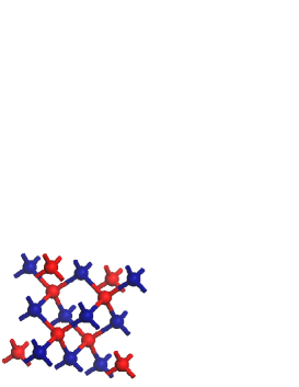
Figure 13: the lattice $\mathcal{L}_{su\left(4\right)}$ with sublattices $\mathcal{A}_{su\left(4\right)}$  (in blue) and $\mathcal{B}_{su\left(4\right)}$  (in red). Each atom has 4 first nearest neighbors, forming a tetrahedron, and 12 second nearest ones.

2) Toy model
This is a lattice QFT on the $\mathcal{L}_{su\left(4\right)}$ with dynamical particles and vacancies. The initial state of the system correspond to the configuration where the sites of the sublattice $\mathcal{A}_{4}$ are occupied by particles and those of the sublattice $\mathcal{B}_{4}$ are unoccupied.

sublattice initial configuration quantum state

$$\mathcal{A}_{{}_{4}}$$ particles at

vacancy at

(4.26)

Then, the particles (vacancies) start to move towards the neighboring sites with movement modeled by hops to first nearest neighbors. Let $A_{\mathbf{r}_{m}}$ and $B_{\mathbf{r}_{m}+\mathbf{v}_{i}}$ be the quantum states describing the particle at $\mathbf{r}_{m}$ and the vacancy at $\mathbf{r}_{m}+\mathbf{v}_{i}$ respectively. Let also $A_{\mathbf{r}_{m}}^{\pm}$ and $B_{\mathbf{r}_{m}+\mathbf{v}_{i}}^{\pm}$ be the corresponding creation and annihilation operators. The hamiltonian describing the hops of the vacancy/particle to the first nearest neighbors is given by

$$H_{{}_{4}}=$$

(4.27)

By performing the Fourier transform of the wave functions $A_{\mathbf{r}_{m}}^{\pm}$, $B_{\mathbf{r}_{m}+\upsilon_{i}}^{\pm}$, we end with the dispersion energy $\pm t\left|\varepsilon_{\mathbf{k}}\right|$ where

$$\varepsilon_{\mathbf{k}}=\sqrt{4+2\mathop{\displaystyle\sum}\limits_{i<j}\cos\left(\mathbf{k.V}_{ij}\right)}$$ ,

(4.28)

and $\mathbf{V}_{ij}$ are as in (4.21-4.22). The Dirac points are located at $\mathbf{k}_{s}=\pm\frac{s\pi}{2a}\sum_{i=1}^{3}\mathbf{\omega}_{i}$ with $s=1,2$.

5 Four dimensional graphene

The so called four dimensional graphene is a QFT model that lives on the 4D hyperdiamond; it has links with lattice quantum chromodynamics (QCD) to be discussed in next section. In this section, we first study the 4D hyperdiamond; then we use the results of previous section to give some physical properties of 4D graphene.

5.1 Four dimensional hyperdiamond

Like in the case of 2D honeycomb, the 4D hyperdiamond may be defined by the superposition of two sublattices $\mathcal{A}_{4}$ and $\mathcal{B}_{4}$ with the following properties:

• sites in $\mathcal{A}_{4}$ and $\mathcal{B}_{4}$ are parameterized by the typical 4d- vectors $\mathbf{r}_{\mathbf{n}}$ with $\mathbf{n}=\left({\small n}_{1}{\small,n}_{2}{\small,n}_{3}{\small,n}_{4}\right)$ and ${\small n}_{i}$’s arbitrary integers. These lattice vectors are expanded as follows

  $$\mathcal{A}_{4}$$: , : ,

  (5.1)

  where $\mathbf{a}_{1},$ $\mathbf{a}_{2},$ $\mathbf{a}_{3},$ $\mathbf{a}_{4}$ are primitive vectors generating these sublattices; and $\mathbf{e}_{5}$ is a shift vector which we describe below.

• the vector $\mathbf{e}_{5}$ is a global vector taking the same value $\forall$ $\mathbf{n}$; it is a shift vector giving the relative positions of the $\mathcal{B}_{4}$ sites with respect to the $\mathcal{A}_{4}$ ones, $\mathbf{e}_{5}\mathbf{=r}_{\mathbf{n}}^{\prime}-\mathbf{r}_{\mathbf{n}}$, $\forall$ $\mathbf{n}$.

The $\mathbf{a}_{l}$’s and $\mathbf{e}_{5}$ vectors can be chosen as

$$\mathbf{a}_{1}=\mathbf{e}_{1}-\mathbf{e}_{5},$$ ,

(5.2)

with

$$\mathbf{e}_{1}^{\mu}$$ ,

,

,

,

(5.3)

and $\mathbf{e}_{5}=-\sum_{i=1}^{4}\mathbf{e}_{i}$. Notice also that the 5 vectors $\mathbf{e}_{1},$ $\mathbf{e}_{2},$ $\mathbf{e}_{3},$ $\mathbf{e}_{4},$ $\mathbf{e}_{5}$ define the first nearest neighbors to $\left(0,0,0,0\right)$ and satisfy the constraint relations,

$$\mathbf{e}_{i}.\mathbf{e}_{i}=1,$$ ,

(5.4)

showing that the $\mathbf{e}_{i}$’s are distributed in a symmetric way since all the angles satisfy $\cos\vartheta_{ij}=\frac{-1}{4}$; see also figure (14) for illustration.

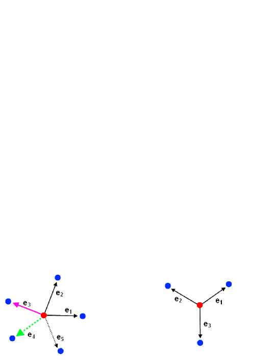
Figure 14: On left the 5  first nearest neighbors in the pristine 4D hyperdiamond with the properties $\left\|\mathbf{e}_{i}\right\|=1$ and $e_{1}+e_{2}+e_{3}+\mathbf{e}_{4}+\mathbf{e}_{5}=0$. On right, the 3 first nearest in pristine 2D graphene with $\left\|\mathbf{e}_{i}\right\|=1$  and $e_{1}+\mathbf{e}_{2}+\mathbf{e}_{3}=0$.

some specific properties
From the figure (14) representing the first nearest neighbors in the 4D hyperdiamond and their analog in 2D graphene, we learn that each $\mathcal{A}_{4}$- type node at $\mathbf{r}_{\mathbf{n}}$, with some attached wave function $A_{\mathbf{r}_{\mathbf{n}}}$, has the following closed neighbors:

• 5 first nearest neighbors belonging to $\mathcal{B}_{4}$ with wave functions $B_{\mathbf{r}_{\mathbf{n}}+d\mathbf{e}_{i}}$; they are given by:

  lattice position attached wave

  $$\ \ \ \mathbf{r}_{\mathbf{n}}+d\mathbf{e}_{1}$$

  (5.5)

  Using this configuration, the typical tight binding hamiltonian describing the couplings between the first nearest neighbors reads as

  $$-t\mathop{\displaystyle\sum}\limits_{\mathbf{r}_{\mathbf{n}}}\mathop{\displaystyle\sum}\limits_{i=1}^{5}A_{\mathbf{r}_{\mathbf{n}}}B_{\mathbf{r}_{\mathbf{n}}+d\mathbf{e}_{i}}^{+}+hc$$ .

  (5.6)

  where $t$ is the hop energy and where $d$ is the lattice parameter.
  Notice that in the case where the wave functions at $\mathbf{r}_{\mathbf{n}}$ and $\mathbf{r}_{\mathbf{n}}+d\mathbf{e}_{i}$ are rather given by two component Weyl spinors

  $$A_{\mathbf{r}_{\mathbf{n}}}^{a}=\left(\begin{array}[]{c}A_{\mathbf{r}_{\mathbf{n}}}^{1}\\ A_{\mathbf{r}_{\mathbf{n}}}^{2}\end{array}\right)$$ , ,

  (5.7)

  together with their adjoints $\bar{A}_{\mathbf{r}_{\mathbf{n}}}^{\dot{a}}$ and $\bar{B}_{\mathbf{r}_{\mathbf{n}}+d\mathbf{e}_{i}}^{a}$, as in the example of 4D lattice QCD to be described in next section, the corresponding tight binding model would be,

  $$-t\mathop{\displaystyle\sum}\limits_{\mathbf{r}_{\mathbf{n}}}\mathop{\displaystyle\sum}\limits_{i=1}^{5}\left[\mathop{\displaystyle\sum}\limits_{\mu=1}^{4}\mathbf{e}_{i}^{\mu}\left(A_{\mathbf{r}_{\mathbf{n}}}^{a}\sigma_{a\dot{a}}^{\mu}\bar{B}_{\mathbf{r}_{\mathbf{n}}+d\mathbf{e}_{i}}^{\dot{a}}\right)\right]+hc$$ .

  (5.8)

  where the $\mathbf{e}_{i}^{\mu}$’s are as in (5.3); and where $\sigma^{1},$ $\sigma^{2},$ $\sigma^{3}$ are the Pauli matrices and $\sigma^{4}=I_{2\times 2}$. Notice moreover that the term $\sum_{i=1}^{5}\mathbf{e}_{i}^{\mu}\left(A_{\mathbf{r}_{\mathbf{n}}}^{a}\sigma_{a\dot{a}}^{\mu}\bar{B}_{\mathbf{r}_{\mathbf{n}}}^{\dot{a}}\right)$ vanishes identically due to $\sum_{i=1}^{5}\mathbf{e}_{i}^{\mu}=0.$

• 20 second nearest neighbors belonging to the same $\mathcal{A}_{4}$ with the wave functions $A_{\mathbf{r}_{\mathbf{n}}+d\left(\mathbf{e}_{i}-\mathbf{e}_{j}\right)}$; they read as

  $${\small r}_{\mathbf{n}}\pm d\left(\mathbf{e}_{1}-\mathbf{e}_{2}\right){\small,}$$

  (5.9)

The 5 vectors $\mathbf{e}_{1},$ $\mathbf{e}_{2},$ $\mathbf{e}_{3},$ $\mathbf{e}_{4},$ $\mathbf{e}_{5}$ are, up to a normalization factor namely $\frac{\sqrt{5}}{2}$, precisely the weight vectors $\mathbf{\lambda}_{0},$ $\mathbf{\lambda}_{1},$ $\mathbf{\lambda}_{2},$ $\mathbf{\lambda}_{3},$ $\mathbf{\lambda}_{4}$ of the 5-dimensional representation of $SU\left(5\right)$; and the 20 vectors $\left(\mathbf{e}_{i}-\mathbf{e}_{j}\right)$ are, up to a scale factor $\frac{\sqrt{5}}{2}$, their roots $\beta_{ij}=\left(\mathbf{\lambda}_{i}-\mathbf{\lambda}_{j}\right)$. We show as well that the particular property $\mathbf{e}_{i}.\mathbf{e}_{j}=-\frac{1}{4}$, which is constant $\forall$ $\mathbf{e}_{i}$ and $\mathbf{e}_{j}$, has a natural interpretation in terms of the Cartan matrix of $SU\left(5\right)$.

2D/4D Correspondence
First notice that a generic bond vector $\mathbf{e}_{i}$ in the hyperdiamond links two sites in the same unit cell of the 4D lattice as shown on the typical coupling term $A_{\mathbf{r}_{\mathbf{n}}}B_{\mathbf{r}_{\mathbf{n}}+d\mathbf{e}_{i}}^{+}$. This property is quite similar to the action of the usual $\gamma^{\mu}$ matrices on 4D (Euclidean) space time spinors which links the components of spinors.
Mimicking the tight binding model of 2D graphene, it has been proposed in (Bedaque et al.,, 2008) a graphene inspired model for 4D lattice QCD. There, the construction relies on the use of the following:

• the naive correspondence between the bond vectors $\mathbf{e}_{i}$ and the $\mathrm{\gamma}^{i}$ matrices

  $$\mathbf{e}_{i}$$ , ,

  (5.10)

  together with

  $$-\mathbf{e}_{5}=\mathbf{e}_{1}+\mathbf{e}_{2}+\mathbf{e}_{3}+\mathbf{e}_{4}$$ ,

  .

  (5.11)

• as in the case of 2D graphene, $\mathcal{A}_{4}$-type sites are occupied by left $\phi_{\mathbf{r}}^{a}$ and right $\bar{\phi}_{\mathbf{r}}^{\dot{a}}$ 2-component Weyl spinors. $\mathcal{B}_{4}$-type sites are occupied by right $\bar{\chi}_{\mathbf{r}+d\mathbf{e}_{i}}^{\dot{a}}$ and left $\chi_{\mathbf{r}+d\mathbf{e}_{i}}^{a}$ Weyl spinors.

        lattice 2D graphene 4D hyperdiamond

  $$\mathcal{A}_{4}$$-sites at  

  where the indices $a=1,2$ and $\dot{a}=\dot{1},\dot{2}$; and where summation over $\mu$ is in the Euclidean sense.

For later use, it is interesting to notice the two following:

(a)

in 2D graphene, the wave functions $A_{\mathbf{r}}$ and $B_{\mathbf{r}+de_{i}}$ describe polarized electrons in first nearest sites of the 2D honeycomb. As the spin up and spin down components of the electrons contribute equally, the effect of spin couplings in 2D graphene is ignored.

(b)

in the 4D hyperdiamond, we have 4+4 wave functions at each $\mathcal{A}_{4}$-type site or $\mathcal{B}_{4}$-type one. These wave functions are given by:

(i)

$\phi^{a}=\left(\phi_{\mathbf{r}_{n}}^{1},\phi_{\mathbf{r}_{n}}^{2}\right)$ and $\bar{\phi}_{\mathbf{r}}^{\dot{a}}=\left(\bar{\phi}_{\mathbf{r}_{n}}^{\dot{1}},\bar{\phi}_{\mathbf{r}_{n}}^{\dot{2}}\right)$ having respectively positive and negative $\mathrm{\gamma}^{5}$ chirality,

(ii)

$\bar{\chi}_{\mathbf{r}+d\mathbf{e}_{i}}^{\dot{a}}=\left(\bar{\chi}_{\mathbf{r}+d\mathbf{e}_{i}}^{\dot{1}},\bar{\chi}_{\mathbf{r}+d\mathbf{e}_{i}}^{\dot{2}}\right)$ and $\chi_{\mathbf{r}+d\mathbf{e}_{i}}^{a}=\left(\chi_{\mathbf{r}+d\mathbf{e}_{i}}^{1},\chi_{\mathbf{r}+d\mathbf{e}_{i}}^{2}\right)$ having respectively negative and positive $\gamma^{5}$ chirality.

By mimicking the 2D graphene study, we have the couplings

$$\mathbf{e}_{i}^{\mu}\sigma_{1\dot{1}}^{\mu}\left(\phi_{\mathbf{r}}^{1}\text{ }\bar{\chi}_{\mathbf{r}+d\mathbf{e}_{i}}^{\dot{1}}\right)$$ ,

,

(5.13)

building the hamiltonian
To describe 4D lattice fermions, one considers 4D space time Dirac spinors together with the following $\gamma^{\mu}$ matrices realizations,

$$\gamma^{1}=\tau^{1}\otimes\sigma^{1}$$ , , ,

, ,

(5.14)

where the $\tau^{i}$’s are the Pauli matrices acting on the sublattice structure of the hyperdiamond lattice,

$$\tau^{1}=\left(\begin{array}[]{cc}0&1\\ 1&0\end{array}\right),$$

(5.15)

The $2\times 2$ matrices $\sigma^{i}$ satisfy as well the Clifford algebra $\sigma^{i}\sigma^{j}+\sigma^{j}\sigma^{i}=2\delta^{ij}I_{2}$ and act through the coupling of left/right Weyl spinors at neighboring sites

$$\phi_{\mathbf{r}}^{a}\sigma_{a\dot{a}}^{\mu}\text{ }\bar{\chi}_{\mathbf{r}+d\frac{\sqrt{5}}{2}\mathbf{\lambda}_{i}}^{\dot{a}}-\chi_{\mathbf{r}}^{a}\bar{\sigma}_{a\dot{a}}^{\mu}\text{ }\bar{\phi}_{\mathbf{r-}d\frac{\sqrt{5}}{2}\mathbf{\lambda}_{i}}^{\dot{a}}=\left(\phi_{\mathbf{r}}\sigma^{\mu}\bar{\chi}_{\mathbf{r}+d\frac{\sqrt{5}}{2}\mathbf{\lambda}_{i}}-\chi_{\mathbf{r}}\bar{\sigma}^{\mu}\bar{\phi}_{\mathbf{r}-d\frac{\sqrt{5}}{2}\mathbf{\lambda}_{i}}\right)$$ (5.16)

where $\sigma^{\mu}=\left(\sigma^{1},\sigma^{2},\sigma^{3},+iI_{2}\right)$ and $\bar{\sigma}^{\mu}=\left(\sigma^{1},\sigma^{2},\sigma^{3},-iI_{2}\right).$ For later use, it is interesting to set

$$\sigma^{\mu}.e_{1}^{\mu}$$ ,

,

(5.17)

and similar relations for the other $\sigma.e_{i}$ and $\bar{\sigma}\mathrm{.}\mathbf{e}_{i}$.

Now extending the tight binding model of 2D graphene to the 4D hyperdiamond; and using the weight vectors $\lambda_{i}$ instead of $e_{i}$, we can build a free fermion action on the 4D lattice by attaching a two-component left-handed spinor $\phi^{a}\left(\mathbf{r}\right)$ and right-handed spinor $\bar{\phi}_{\mathbf{r}}^{\dot{a}}$ to each $A_{4}$-node $r$, and a right-handed spinor $\bar{\chi}_{\mathbf{r}+d\frac{\sqrt{5}}{2}\mathbf{\lambda}_{i}}^{\dot{a}}$ and left-handed spinor $\chi_{\mathbf{r}+d\frac{\sqrt{5}}{2}\mathbf{\lambda}_{i}}^{a}$ to every $B_{4}$-node at $r+d\frac{\sqrt{5}}{2}\lambda_{i}$.
The hamiltonian, describing hopping to first nearest-neighbor sites with equal probabilities in all five directions $\mathbf{\lambda}_{i}$, reads as follows:.

$$H_{4}$$ .

(5.18)

Expanding the various spinorial fields $\xi_{\mathbf{r\pm v}}$ in Fourier sums as $\int\frac{d^{4}k}{\left(2\pi\right)^{4}}e^{-i\mathbf{k.r}}\left(e^{\mp i\mathbf{k.v}}\xi_{\mathbf{k}}\right)$ with $\mathbf{k}$ standing for a generic wave vector in the reciprocal lattice, we can put the field action $H_{4}$ into the form

$$H_{4}$$

(5.19)

where we have set

$$D$$ ,

(5.20)

with

$$D_{l}=\mathop{\displaystyle\sum}\limits_{\mu=1}^{4}\sigma^{\mu}\lambda_{l}^{\mu}=\left(\begin{array}[]{cc}\lambda_{l}^{3}+i\lambda_{l}^{4}&\lambda_{l}^{1}-i\lambda_{l}^{2}\\ \lambda_{l}^{1}+i\lambda_{l}^{2}&\lambda_{l}^{3}-i\lambda_{l}^{4}\end{array}\right)$$ ,

(5.21)

and $p_{l}=\mathbf{k}.\lambda_{l}=\sum_{\mu}k_{\mu}\lambda_{l}^{\mu}$. Similarly we have

$$\bar{D}$$ .

(5.22)

5.2 Energy dispersion and zero modes

To get the dispersion energy relations of the 4 waves components $\phi_{\mathbf{k}}^{1}$, $\phi_{\mathbf{k}}^{2}$, $\chi_{\mathbf{k}}^{1},$ $\chi_{\mathbf{k}}^{2}$ and their corresponding 4 holes, one has to solve the eigenvalues of the Dirac operator (5.19). To that purpose, we first write the 4-dimensional wave equation as follows,

$$\left(\begin{array}[]{cc}0&-iD\\ i\bar{D}&0\end{array}\right)\left(\begin{array}[]{c}\phi_{\mathbf{k}}\\ \chi_{\mathbf{k}}\end{array}\right)$$ ,

(5.23)

where $\phi_{\mathbf{k}}=\left(\phi_{\mathbf{k}}^{1},\phi_{\mathbf{k}}^{2}\right)$, $\chi_{\mathbf{k}}=\left(\chi_{\mathbf{k}}^{1},\chi_{\mathbf{k}}^{2}\right)$ are Weyl spinors and where the $2\times 2$ matrices $D$, $\bar{D}$ are as in eqs(5.20,5.22). Then determine the eigenstates and eigenvalues of the $2\times 2$ Dirac operator matrix by solving the following characteristic equation,

$$\det\left(\begin{array}[]{cccc}-E&0&D_{11}&D_{12}\\ 0&-E&D_{21}&D_{22}\\ \bar{D}_{11}&\bar{D}_{21}&-E&0\\ \bar{D}_{12}&\bar{D}_{22}&0&-E\end{array}\right)$$

(5.24)

from which one can learn the four dispersion energy eigenvalues $E_{1}\left(\mathbf{k}\right)$, $E_{2}\left(\mathbf{k}\right)$, $E_{3}\left(\mathbf{k}\right)$, $E_{4}\left(\mathbf{k}\right)$ and therefore their zeros.

1) computing the energy dispersion
An interesting way to do these calculations is to act on (5.23) once more by the Dirac operator to bring it to the following diagonal form

$$\left(\begin{array}[]{cc}D\bar{D}&0\\ 0&D\bar{D}\end{array}\right)\left(\begin{array}[]{c}\phi_{\mathbf{k}}\\ \chi_{\mathbf{k}}\end{array}\right)$$ .

(5.25)

Then solve separately the eigenvalues problem of the 2-dimensional equations $D\bar{D}\phi_{\mathbf{k}}=E^{2}\phi_{\mathbf{k}}$ and $\bar{D}D\chi_{\mathbf{k}}=E^{2}\chi_{\mathbf{k}}$. To do so, it is useful to set

$$u\left(\mathbf{k}\right)=\vartheta^{1}+i\vartheta^{2}$$ ,

(5.26)

with $\vartheta^{\mu}=\sum_{l}\lambda_{l}^{\mu}\exp(id\frac{\sqrt{5}}{2}k.\lambda_{l})$. Notice that in the continuous limit, we have $\vartheta^{\mu}\rightarrow id\frac{\sqrt{5}}{2}\mathbf{k}^{\mu}$,

$$u\left(\mathbf{k}\right)\rightarrow id\frac{\sqrt{5}}{2}\left(\mathbf{k}^{1}+i\mathbf{k}^{2}\right)$$, .

(5.27)

Substituting (5.26) back into (5.20) and (5.22), we obtain the following expressions,

$${\small D\bar{D}=}\left(\begin{array}[]{cc}\left|u\right|^{2}{\small+}\left|v\right|^{2}&{\small 2\bar{u}v}\\ {\small 2u\bar{v}}&\left|u\right|^{2}{\small+}\left|v\right|^{2}\end{array}\right),$$

(5.28)

By solving the characteristic equations of these $2\times 2$ matrix operators, we get the eigenstates $\phi_{\mathbf{k}}^{a\prime}$, $\chi_{\mathbf{k}}^{a\prime}$ with their corresponding eigenvalues $E_{\pm}^{2}$,

         eigenstates          eigenvalues

$$\phi_{\mathbf{k}}^{1\prime}=$$

(5.29)

By taking square roots of $E_{\pm}^{2}$, we obtain 2 positive and 2 negative dispersion energies; these are

$$E_{\pm}=+\sqrt{\left(\left|u\right|\pm\left|v\right|\right)^{2}},$$

(5.30)

which correspond respectively to particles and the associated holes.

2) determining the zeros of $E_{\pm}$ and $E_{\pm}^{\ast}$
From the above energy dispersion relations, one sees that the zero modes are of two kinds: $E_{+}^{2}=0,$ $E_{-}^{2}=0$; and $E_{-}^{2}=0$ but $E_{+}^{2}=E_{+\min}^{2}\neq 0$. Let us consider the case $E_{+}^{2}=E_{-}^{2}=0$; in this situation the zero modes are given by those wave vectors $\mathbf{K}_{F}$ solving the constraint relations $u\left(\mathbf{K}_{F}\right)=v\left(\mathbf{K}_{F}\right)=0$. These constraints can be also put in the form

$$\lambda_{0}^{\mu}e^{id\frac{\sqrt{5}}{2}\mathbf{K}_{F}.\mathrm{\lambda}_{0}}+\lambda_{1}^{\mu}e^{id\frac{\sqrt{5}}{2}\mathbf{K}_{F}.\mathrm{\lambda}_{1}}+$$

(5.31)

for all values of $\mu=1,2,3,4$, or equivalently like $d\frac{\sqrt{5}}{2}K_{F}.\lambda_{l}=\frac{2\pi}{5}N+2\pi N_{l}.$ Notice that setting $\mathbf{k}=\mathbf{K}_{F}+\mathbf{q}$ with small $q=\left\|\mathbf{q}\right\|$ and expanding $D$ and $\bar{D}$, eq(5.23) gets reduced to the following familiar wave equation in Dirac theory

$$\frac{d\sqrt{5}}{2}\mathop{\displaystyle\sum}\limits_{\mu=1}^{4}\mathbf{q}_{\mu}\left(\begin{array}[]{cc}0&\sigma^{\mu}\\ \bar{\sigma}^{\mu}&0\end{array}\right)\left(\begin{array}[]{c}\phi_{\mathbf{k}}\\ \bar{\chi}_{\mathbf{k}}\end{array}\right)$$ .

(5.32)

6 Graphene and lattice QCD

In this section, we would like to deepen the connection between 2D graphene and 4D lattice QCD. This connection has been first noticed by M.Creutz (Creutz,, 2008) and has been developed by several authors seen its convenience for numerical simulations in QCD .

6.1 More on link graphene/lattice QCD

2D graphene has some remarkable properties that can be used to simulate 4D lattice QCD. Besides chirality, one of the interesting properties is the existence of two Dirac points that can be interpreted as the light quarks up and down. This follows from the study of the zero modes of the $2\times 2$ Dirac operator which corresponds also to solve the vanishing of the following energy dispersion relation

$$\mathop{\displaystyle\sum}\limits_{l=1}^{l}\cos ak_{l}+i\mathop{\displaystyle\sum}\limits_{l=1}^{l}\sin ak_{l}=0$$ ,

(6.1)

which has two zeros as given by (2.22).
To make contact with lattice QCD, we start by recalling the usual 4D hamiltonian density of a free Dirac fermion $\Psi=\left(\psi^{1},\psi^{2},\bar{\chi}_{\dot{1}},\bar{\chi}_{\dot{2}}\right)$ living in a euclidian space time,

$$H=\frac{1}{2}\int d^{4}x\left(\mathop{\displaystyle\sum}\limits_{\mu=1}^{4}\bar{\Psi}\left(x\right)\gamma^{\mu}\frac{\partial\Psi\left(x\right)}{\partial x^{\mu}}+hc\right),$$ (6.2)

where $\mathrm{\gamma}^{\mu}$ are the usual $4\times 4$ Dirac matrices given by (5.14). Then, we discretize this energy density H by thinking about the spinorial waves $\Psi\left(x^{1},...,x^{4}\right)$ as $\Psi_{\mathbf{r}_{n}}$ living at the $\mathbf{r}_{n}$-nodes of a four dimensional lattice $\mathbb{L}_{4}$ and its space time gradient $\frac{\partial\Psi\left(x\right)}{\partial x^{\mu}}$ like $\frac{1}{a}\left(\Psi_{\mathbf{r}_{n}+a\mathbf{\mu}}-\Psi_{\mathbf{r}_{n}}\right)$. The field $\Psi_{\mathbf{r}_{n}+a\mathbf{\mu}}$ is the value of the Dirac spinor at the lattice position $\mathbf{r}_{n}+a\mathbf{\mu}$ with the unit vectors $\mathbf{\mu}$ giving the four relative positions of the first nearest neighbors of $\mathbf{r}_{n}$. Putting this discretization back into (6.2), we end with the free fermion model

$$H=\frac{1}{2a}\mathop{\displaystyle\sum}\limits_{\mathbf{r}_{n}}\left(\mathop{\displaystyle\sum}\limits_{\mu=1}^{4}\left[\bar{\Psi}_{\mathbf{r}_{n}}\gamma^{\mu}\Psi_{\mathbf{r}_{n}+a\mathbf{\mu}}-\bar{\Psi}_{\mathbf{r}_{n}+a\mathbf{\mu}}\gamma^{\mu}\Psi_{\mathbf{r}_{n}}\right]\right)$$ .

(6.3)

The extra two term $\bar{\Psi}_{\mathbf{r}_{n}}\Gamma\Psi_{\mathbf{r}_{n}}$ and $\left(\bar{\Psi}_{\mathbf{r}_{n}}\Gamma\Psi_{\mathbf{r}_{n}}\right)^{+}$ with $\Gamma=\frac{1}{2}\sum_{\mu}\gamma^{\mu}$ cancel each other because of antisymmetry of the spinors. Clearly, this hamiltonian looks like the tight binding hamiltonian describing the electronic properties of the 2D graphene; so one expects several similarities for the two systems.
Mapping the hamiltonian (6.3) to the Fourier space, we get $H=\sum_{\mathbf{k}}\left(\bar{\Psi}_{\mathbf{k}}\mathcal{D}\Psi_{\mathbf{k}}\right)$ with Dirac operator $\mathcal{D}=\frac{i}{a}\sum_{\mu=1}^{4}\gamma^{\mu}\sin\left(ak_{\mu}\right),$where we have set $k_{\mu}=\left(\mathbf{k.\mu}\right)$; giving the wave vector component along the $\mathbf{\mu}$-direction. The $\mathcal{D}$- operator is a $4\times 4$ matrix that depends on the wave vector components $\left(k_{1},k_{2},k_{3},k_{4}\right)$ and has $2^{4}$ zeros located as

$$k_{1}=0,\text{ }\frac{\pi}{a}$$ ; ; ; .

(6.4)

However, to apply these formalism to 4D lattice QCD, the number of the zero modes of the Dirac operator should be two in order to interpret them as the light quarks up and down. Following (Creutz,, 2008), this objective can be achieved by modifying (6.3) so that the Dirac operator takes the form

$$\mathcal{D}=\frac{i}{a}\mathop{\displaystyle\sum}\limits_{\mu=1}^{4}\gamma^{\mu}\sin\left(ak_{\mu}\right)+\frac{i}{a}\mathop{\displaystyle\sum}\limits_{\mu=1}^{4}\gamma^{\prime\mu}\cos\left(ak_{\mu}\right)$$ (6.5)

where $\mathrm{\gamma}^{\prime\mu}$ is some $4\times 4$ matrix that is introduced in next subsection.

6.2 Boriçi-Creutz fermions

Following (Capitani et al., 2009 a, ; Capitani et al., 2009 b, ) and using the 4-component Dirac spinors $\Psi_{\mathbf{r}}=\left(\phi_{\mathbf{r}}^{a},\bar{\chi}_{\mathbf{r}}^{\dot{a}}\right)$, the Boriçi-Creutz (BC) lattice action of free fermions reads in the position space, by dropping mass term $m_{0}$, as follows:

$$H_{BC}$$

(6.6)

where, for simplicity, we have dropped out gauge interactions; and where $\Upsilon^{\mu}=\gamma^{\mu}+i\gamma^{\prime\mu}$; which is a kind of complexification of the Dirac matrices.
Moreover, the matrix $\Gamma$ appearing in the last term is a $4\times 4$ matrix linked to $\gamma^{\mu}$, $\gamma^{\prime\mu}$ as follows:

$$\gamma^{\prime\mu}=\Gamma-\gamma^{\mu},$$ , ,

(6.7)

Mapping (6.6) to the reciprocal space, we have

$$H_{BC}$$

(6.8)

where the massless Dirac operator $\mathcal{D}_{BC}$ is given by

$$\mathcal{D}_{BC}=$$

.

(6.9)

Upon using $\Upsilon_{\mu}+\bar{\Upsilon}_{\mu}=2\gamma_{\mu}$ and $\Upsilon_{\mu}-\bar{\Upsilon}_{\mu}=2i\gamma_{\mu}^{\prime}$, we can put $\mathcal{D}_{BC}$ in the form

$$\mathcal{D}_{BC}=D_{\mathbf{k}}+\bar{D}_{\mathbf{k}}-\frac{2i}{a}\Gamma$$ (6.10)

with

$$D_{\mathbf{k}}=\frac{i}{a}\left(\mathop{\displaystyle\sum}\limits_{\mu=1}^{4}\gamma^{\mu}\sin ak_{\mu}\right)$$ , ,

(6.11)

where $k_{\mu}=\mathbf{k}.\mathbf{\mu}$. In the next subsection, we will derive the explicit expression of these $k_{\mu}$’s in terms of the weight vectors $\mathbf{\lambda}_{l}$ of the 5-dimensional representation of the $SU\left(5\right)$ symmetry as well as useful relations.
The zero modes of $\mathcal{D}_{BC}$ are points in the reciprocal space; they are obtained by solving $\mathcal{D}_{BC}=0$; which leads to the following condition

$$\mathop{\displaystyle\sum}\limits_{\mu=1}^{4}\mathrm{\gamma}^{\mu}\left(\sin aK_{\mu}-\cos aK_{\mu}\right)-\Gamma\left(2-\mathop{\displaystyle\sum}\limits_{\mu=1}^{4}\cos aK_{\mu}\right)=0$$ .

(6.12)

This condition is a constraint relation on the wave vector components $K_{\mu}$; it is solved by the two following wave vectors:

point $$K_{BC}$$ : ,

point : ,

(6.13)

that are interpreted in lattice QCD as associated with the light quarks up and down.
Notice that if giving up the $\gamma_{\mu}^{\prime}$- terms in eqs(6.6-6.8); i.e $\gamma_{\mu}^{\prime}\rightarrow 0$, the remaining terms in $D_{BC}$ namely $D_{\mathbf{k}}\sim\gamma^{\mu}\sin aK_{\mu}$ have 16 zero modes given by the wave components $K_{\mu}=0,\pi$. By switching on the $\gamma_{\mu}^{\prime}$-terms, 14 zeros are removed.

6.3 Hyperdiamond model

The hamiltonian $H_{BC}$ is somehow very particular; it let suspecting to hide a more fundamental property which can be explicitly exhibited by using hidden symmetries. To that purpose, notice that the price to pay for getting a Dirac operator with two zero modes is the involvement of the complexified Dirac matrices $\Upsilon^{\mu},$ $\bar{\Upsilon}^{\mu}$ as well as the particular matrix $\Gamma$. Despite that it violates explicitly the $SO\left(4\right)$ Lorentz symmetry since it can be written as

$$\Gamma=\frac{1}{2}\mathop{\displaystyle\sum}\limits_{\mu=1}^{4}\gamma^{\mu}\upsilon_{\mu},$$

(6.14)

the matrix $\Gamma$ plays an important role in studying the zero modes. The expression of the matrix $\Gamma$ (6.7) should be thought of as associated precisely with the solution of the constraint relation $2\Gamma-\sum_{\mu=1}^{4}\gamma^{\mu}=0$ that is required by a hidden symmetry of the BC model. This invariance is precisely the $SU\left(5\right)$ symmetry of the 4D hyperdiamond to be identified below. Moreover, the BC hamiltonian $H_{BC}$ lives on a 4D lattice $\mathbb{L}_{4}^{BC}$ generated by $\mathbf{\mu\equiv v}_{\mu}$; i.e the vectors

$$\mathbf{v}_{1}\mathbf{=}\left(\begin{array}[]{c}\mathbf{v}_{1}^{x}\\ \mathbf{v}_{1}^{y}\\ \mathbf{v}_{1}^{z}\\ \mathbf{v}_{1}^{t}\end{array}\right),$$

(6.15)

These $\mathbf{\mu}$-vectors look somehow ambiguous to be interpreted both by using the analogy with 4D graphene prototype; and also from the $SU\left(5\right)$ symmetry view. Indeed, to each site $\mathbf{r}\in\mathbb{L}_{4}^{BC}$ there should be 5 first nearest neighbors that are rotated by $SU\left(5\right)$ symmetry. But from the BC hamiltonian we learn that the first nearest neighbors to each site $\mathbf{r}$ are:

$$\mathbf{r}$$ .

(6.16)

The fifth missing one, namely $\mathbf{r}\rightarrow\mathbf{r+}a\mathbf{v}_{5}$ may be interpreted in the BC fermions as associated with the extra term involving the matrix $\Gamma$. To take into account the five nearest neighbors, we have to use the rigorous correspondence $\Gamma^{\mu}\rightarrow\mathbf{v}_{\mu}$ and $\Gamma^{5}\rightarrow\mathbf{v}_{5}$ which can be also written in a combined form as follows $\Gamma^{M}\rightarrow\mathbf{v}_{M}$ with $\Gamma^{M}=\left(\Gamma^{\mu},\Gamma^{5}\right)$ and $\mathbf{v}_{M}=\left(\mathbf{v}_{\mu},\mathbf{v}_{5}\right).$ Because of the $SU\left(5\right)$ symmetry properties, we also have to require the condition $\mathbf{v}_{1}+\mathbf{\mathbf{v}_{2}+\mathbf{v}_{3}+\mathbf{v}_{4}+v}_{5}=0$ characterizing the 5 first nearest neighbors. To determine the explicit expressions of the matrices $\Gamma_{M}$ in terms of the usual Dirac ones, we modify the BC model (6.6) as follows

$$H_{BC}^{\prime}$$ ,

(6.17)

exhibiting both $SO\left(4\right)$ and $SU\left(5\right)$ symmetries and leading to the following free Dirac operator

$$\mathcal{D}=$$

(6.18)

where $k_{M}=\mathbf{k.v}_{M}$ and where $\Pi_{M=1}^{5}\left(e^{iak_{M}}\right)=1$, $\sum_{M=1}^{5}k_{M}=0$ expressing the conservation of total momenta at each lattice site. Equating with (6.9-6.10-6.11), we get the identities

$$\Upsilon_{\mu}+\bar{\Upsilon}_{\mu}=\Gamma_{\mu}+\bar{\Gamma}_{\mu},$$

(6.19)

and

$$\frac{i}{2a}\left(\Gamma_{5}+\bar{\Gamma}_{5}\right)\sin\left(ak_{5}\right)+\frac{1}{2a}\left(\Gamma_{5}-\bar{\Gamma}_{5}\right)\cos\left(ak_{5}\right)=-\frac{4i}{2a}\Gamma$$ .

(6.20)

Eqs(6.19) are solved by $\Gamma_{\mu}=\Upsilon_{\mu}$; that is $\Gamma_{\mu}=\gamma^{\mu}+i\left(\Gamma-\gamma^{\mu}\right)$ while

$$\Gamma_{5}=-2i\Gamma$$ for ,

for .

(6.21)

where $k_{5}=-\left(k_{1}+k_{2}+k_{3}+k_{4}\right)$. In this 5-dimensional approach, the ambiguity in dealing with the $\mathbf{\mu}$-vectors is overcome; and the underlying $SO\left(4\right)$ and $SU\left(5\right)$ symmetries of the model in reciprocal space are explicitly exhibited.

7 Conclusion and comments

Being a simple lattice-carbon based structure with delocalized electrons, graphene has been shown to exhibit several exotic physical properties and chemical reactions leading to the synthesis of graphene type derivatives such as graphAne and graphOne. In this book chapter, we have shown that graphene has also very remarkable hidden symmetries that capture basic physical properties; one of these symmetries is the well known $SU\left(2\right)$ invariance of the unit cells that plays a crucial role in the study of the electronic properties using first principle calculations. Another remarkable hidden invariance, which has been developed in this work, is the SU$\left(3\right)$ symmetry that captures both crystallographic and physical properties of the graphene. For instance, first nearest neighbors form 3-dimensional representations of $SU\left(3\right)$; and the second nearest neighbor ones transform in its adjoint. Moreover, basic constraint relations like $\mathbf{\upsilon}_{1}+\mathbf{\upsilon}_{2}+\mathbf{\upsilon}_{3}=0$ is precisely a $SU\left(3\right)$ group property; and its solutions are exactly given by group theory. Furthermore, the location of the Dirac zero modes of graphene is also captured by $SU\left(3\right)$ seen that these points are given by $\pm\frac{2\pi}{3d}\mathbf{\alpha}_{1},$ $\pm\frac{2\pi}{3d}\mathbf{\alpha}_{2},$ $\pm\frac{2\pi}{3d}\mathbf{\alpha}_{3}$ where the $\mathbf{\alpha}_{i}$’s are the $SU\left(3\right)$ roots that generate the reciprocal space.
On the other hand, from $SU\left(3\right)$ group theory’s point of view, graphene has cousin systems with generic $SU\left(N\right)$ symmetries where the integer $N$ takes the values $2,3,4,...$. The leading graphene cousin systems are linear molecules with hidden SU$\left(2\right)$ invariance; this is precisely the case of poly-acetylene, cumulene and poly-yne studied in section 4. The graphene cousin systems with hidden SU$\left(4\right)$ and SU$\left(5\right)$ symmetries are given by 3D diamond; and 4D hyperdiamond which has an application in 4D- lattice QCD.
Finally, it is worth to mention that the peculiar and unique properties of graphene are expected to open new areas of applications due to its important electronic, spintronic, mechanical and optical properties. The challenge is find low-cost-processes for producing graphene and graphene-based structures and to tune its properties to the targeted applications such as the replacement of silicon in the field of new-type of semiconductors and new electronics, new data-storage devices, new materials with exceptional mechanical properties and so on.
Various attempts are also made to incorporate other atoms within the structure of graphene or combine the graphene-based structures with other materials in sandwich type structure or in chemical way by binding it to various molecules with divers topologies and functionalities.

References

- Bedaque et al., (2008) P. F. Bedaque, M. I. Buchoff, B. C. Tiburzi, A. Walker-Loud, Broken Symmetries from Minimally Doubled Fermions, Phys. Lett. B, 662 (2008), 449–457,
- Boriçi, (2008) A. Boriçi, Creutz fermions on an orthogonal lattice, Phys. Rev. D, 78 (October 2008) 074504-074506,
- (3) S. Capitani, J. Weber, H. Wittig, Minimally doubled fermions at one loop, Phys. Lett. B 681, (2009), 105-112,
- (4) S. Capitani, J. Weber, H. Wittig, Minimally doubled fermions at one-loop level, Proceedings of Science, The XXVII International Symposium on Lattice Field Theory - LAT2009, 1-7, (July 26-31 2009), Peking University, Beijing, China,
- Capitani et al., (2010) S. Capitani, M. Creutz, J. Weber, H.Wittig, J. High Energy Phys, Renormalization of minimally doubled fermions, Volume 2010, Number 9, ,2010, 27,
- Castro-Neto et al., (2009) A.H. Castro-Neto, F. Guinea, N. M. R. Peres, K. S. Novoselov and A. K. Geim, The electronic properties of graphene, Rev. Mod. Phys. 81, (January 2009), 109–162,
- Chakrabarti et al., (2009) D. Chakrabarti, S.Hands, A.Rago, Topological Aspects of Fermions on a Honeycomb Lattice, J. High Energy Phys, Volume 2009, Issue 06 (June 2009) 060,
- Charlier et al., (1991) J. C. Charlier, X. Gonze, J. P. Michenaud, Phys. Rev. B. 43, (1991), 4579–4589,
- Cortijo & Vozmediano, (2009) A. Cortijo, M A. H. Vozmediano, Nucl.Phys.B 807, (2009), 659-660,
- Creutz, (2008) M. Creutz, Four-dimensional graphene and chiral fermions, J.High Energy Phys, Volume 2008, Issue 04 (April 2008) 017,
- Di Pierro, (2005) M. Di Pierro, An Algorithmic Approach to Quantum Field Theory, Int.J.Mod.Phys.A, 21, (2006), 405-448,
- Drissi et al., (2010) L.B Drissi, E.H Saidi, M.Bousmina, Electronic properties and hidden symmetries of graphene, Nucl Phys B, Vol 829, (April 2010), 523-533,
- (13) L.B Drissi, E.H Saidi, M.Bousmina, Four dimensional graphene
- (14) L.B Drissi, E.H Saidi, M.Bousmina, Graphene, Lattice QFT and Symmetries, J. Math. Phys. 52, (February 2011), 022306-022319,
- Drissi & Saidi, (2011) L. B Drissi, E. H Saidi, On Dirac Zero Modes in Hyperdiamond Model, ISSN arXiv:1103.1316,
- Ferrante & Guralnik, (2006) D. D. Ferrante, G. S. Guralnik, Mollifying Quantum Field Theory or Lattice QFT in Minkowski Spacetime and Symmetry Breaking, ISSN arXiv:hep-lat/0602013,
- Geim & Novoselov, (2007) A. K. Geim, K. S. Novoselov, The rise of graphene, Nature Materials, 6, 183, (2007), 183-191,
- Giuliani et al., (2010) A. Giuliani, V. Mastropietro, M. Porta, Lattice gauge theory model for graphene, Phys.Rev.B, 82, (September 2010), 121418-121421(R),
- Giritet et al., (2009) C. O. Giritet, J C. Meyer, R. Erni, M D. Rossell, C. Kisielowski, L. Yang, C-H Park, M. F. Crommie, M L. Cohen, S G. Louie, A. Zettl, Graphene at the Edge: Stability and Dynamics, Science, 23, (March 2009), 1705-1708,
- Goerbig et al., (2006) M.O. Goerbig, R. Moessner, B. Doucot, Electron interactions in graphene in a strong magnetic field, Phys. Rev. B, 74, (October 2006), 161407-161410,
- Haldane, (1983) F. D. M. Haldane, Fractional Quantization of the Hall Effect: A Hierarchy of Incompressible Quantum Fluid States, Phys. Rev. Lett. 51, (August 1983), 605-608,
- Haldane, (1988) F. D. M. Haldane, Model for a Quantum Hall Effect without Landau Levels: Condensed-Matter Realization of the "Parity Anomaly", Phys. Rev. Lett. 61, (October 1988), 2015-2018,
- Jackiw & Pi, (2007) R. Jackiw, S.-Y. Pi, Chiral Gauge Theory for Graphene, Phys. Rev. Lett. 98 (June 2007), 266402-266405,
- Jackiw & Pi, (2008) R. Jackiw, S.-Y. Pi, Persistence of zero modes in a gauged Dirac model for bilayer graphene, Phys. Rev. B, 78, (October 2008), 132104-132106,
- Jun, (2008) S. Jun, Density-functional study of edge stress in graphene, Phys. Rev. B, 78, (August 2008), 073405-073408,
- Kimura & Misumi, (2010) T. Kimura, T. Misumi, Characters of Lattice Fermions Based on the Hyperdiamond Lattice, Prog. Theor. Phys, 124 (2010), 415-432,
- Koskinen et al., (2008) P. Koskinen, S. Malola, H. Hakkinen, Self-Passivating Edge Reconstructions of Graphene, Phys.Rev. Lett., 101, (September 2008), 115502-115505,
- McCann & Falko, (2006) E. McCann, V.I. Falko, Landau-Level Degeneracy and Quantum Hall Effect in a Graphite Bilayer, Phys. Rev. Lett. 96 (June 2006), 086805-086808,
- Nomura & Mac Donald, (2006) K. Nomura, A. H. Mac Donald, Quantum Hall Ferromagnetism in Graphene, Phys. Rev. Lett. 96, (June 2006), 256602-256605,
- Novoselov et al., (2004) K. S. Novoselov, A. K. Geim, S. V. Morozov, D. Jiang, Y. Zhang, S. V. Dubonos, I. V. Grigorieva, A. A. Firsov, (2004). Electric Field Effect in Atomically Thin Carbon Films, Science, 306, 5696, (October 2004), 666-669,
- Novoselov et al., (2006) K. S. Novoselov, E. McCann, S. V. Morozov, V. I. Fal’ko, M. I. Katsnelson, U. Zeitler, D. Jiang, F. Schedin, A. K. Geim, Unconventional quantum Hall effect and Berry’s phase of 2pi in bilayer graphene, Nat. Phys. 2 (2006),177-180,
- Ohta et al., (2006) T. Ohta, A. Bostwick, T. Seyller, K. Horn, E. Rotenberg, Controlling the Electronic Structure of Bilayer Graphene, Science, 313, 5789 (August 2006), 951-954,
- Ohta et al., (2007) T. Ohta, A. Bostwick, J. L. McChesney, T. Seyller, K. Horn, E. Rotenberg, Interlayer Interaction and Electronic Screening in Multilayer Graphene Investigated with Angle-Resolved Photoemission Spectroscopy, Phys. Rev. Lett. 98 (May 2007), 206802-206805,
- Wallace, (1947) P.R Wallace, The Band Theory of Graphite, Phys Rev, 71, (May 1947), 622–634,
- Slonczewski & Weiss, (1958) J. C. Slonczewski and P. R. Weiss, Band Structure of Graphite, Phys. Rev. 109, (January 1958), 272–279,
- Semenoff, (1984) G.V. Semenoff, Condensed-Matter Simulation of a Three-Dimensional Anomaly, Phys. Rev. Lett. 53, (December 1984), 2449–2452,
- Zheng & Ando, (2002) Y. Zheng and T. Ando, Hall conductivity of a two-dimensional graphite system, Phys. Rev. B 65, (June 2002), 245420-245430,
- Zhang et al., (2005) Y. Zhang, Y-Wen Tan, H L. Stormer, P. Kim, Experimental observation of the quantum Hall effect and Berry’s phase in graphene, Nature 438, (November 2005), 201-204,
- Zhang et al., (2006) Y. Zhang, Z. Jiang, J. P. Small, M. S. Purewal, Y.-W. Tan, M. Fazlollahi, J. D. Chudow, J. A. Jaszczak, H. L. Stormer, and P. Kim, Landau-Level Splitting in Graphene in High Magnetic Fields, Phys. Rev. Lett. 96, (April 2006), 136806-136809.