Characterization of the Dynamics of Glass-forming Liquids from the Properties of the Potential Energy Landscape

Abstract

We develop a framework for understanding the difference between strong and fragile behavior in the dynamics of glass-forming liquids from the properties of the potential energy landscape. Our approach is based on a master equation description of the activated jump dynamics among the local minima of the potential energy (the so-called inherent structures) that characterize the potential energy landscape of the system. We study the dynamics of a small atomic cluster using this description as well as molecular dynamics simulations and demonstrate the usefulness of our approach for this system. Many of the remarkable features of the complex dynamics of glassy systems emerge from the activated dynamics in the potential energy landscape of the atomic cluster. The dynamics of the system exhibits typical characteristics of a strong supercooled liquid when the system is allowed to explore the full configuration space. This behavior arises because the dynamics is dominated by a few lowest-lying minima of the potential energy and the potential energy barriers between these minima. When the system is constrained to explore only a limited region of the potential energy landscape that excludes the basins of attraction of a few lowest-lying minima, the dynamics is found to exhibit the characteristics of a fragile liquid.

I Introduction

In the supercooled state, glass-forming liquids exhibit many fascinating features CAAngell1 ; WKob ; PGDebenedetti in its dynamic behavior, such as multistage, non-exponential decay of fluctuations and a rapid growth of relaxation times with decreasing temperature. In these aspects, glassy systems challenge us with many interesting issues and questions which are not well resolved theoretically.

A popular phenomenological characterization of the dynamics of glassy systems, proposed by Angell, CAAngell1 ; WKob ; PGDebenedetti ; CAAngell2 is the classification of the dynamics as strong or fragile. It classifies different glass formers on the basis of the temperature dependence of their viscosity $\eta$ or their structural relaxation time $\tau$. Quite generally, the rapid growth of $\tau$ with temperature $T$ can be represented by a generalized Arrhenius form, $\tau(T)\sim\exp{(E_{b}(T)/k_{B}T)}$ with an effective temperature dependent activation energy $E_{b}(T)$. For strong systems, this activation energy is essentially independent of temperature while fragile systems exhibit a strong temperature dependence of this quantity: it increases as $T$ is decreased. This implies that the relaxation mechanism is independent of temperature for the first type of systems, whereas for the other type, it depends on $T$. Although various measures of the extent of fragility exist in literature GRuocco1 in terms of the slope of the $\ln(\tau)$ vs. $1/T$ plot, the quantitative distinction between strong and fragile liquids at a microscopic level is not fully understood yet.

Following Goldstein MGoldstein1 , a widely accepted way of looking at glassy dynamics is to view the dynamical evolution of the system in terms of the motion of a state point in configuration space, specified by $3N$ coordinates for an $N$ particles system, over its potential energy surface, often referred to as potential energy landscape (PEL) DJWales1 . For glass-forming liquids and other disordered systems such as spin glasses KBinder in general, a generic feature of the PEL is the existence of a large number of local minima in it, so that the potential energy surface has very rough topography. At low temperature, in the supercooled regime, the system visits the neighborhood of a local minimum for very long times and makes occasional jumps to other minima close to the initial one over the barriers separating them. Following this description, Stillinger and Weber FHStillinger1 ; FHStillinger2 ; FHStillinger3 showed that a useful approach towards the understanding of the low-temperature properties of such system with a rugged PEL is to divide the configuration space into basins of attraction of the local minima and then formulate a statistical description in terms of the distributions of different properties of these local minima, denoted as inherent structures (IS), and their basins of attraction. Stillinger also suggested FHStillinger4 a rationale for the difference between strong and fragile liquids based on the PEL viewpoint. According to his idea, strong liquids have a uniformly rough PEL and there is not much variation in the values of the energy barriers separating different inherent structures. On the contrary, the PEL of fragile liquids have non-uniform roughness. At high temperatures, the system explores a PEL with nearly uniform roughness due to its high kinetic energy, but at lower temperatures it explores the deep valleys with very different energy barriers, giving rise to a temperature-dependent average barrier height. The work of Sastry et al. SSastry1 demonstrated the usefulness of this description, although the understanding of the dynamics in this approach still remains qualitative to a large extent.

After early work FHStillinger1 ; FHStillinger2 on the implementation of a description based on inherent structures by supplementing conventional Molecular Dynamics (MD) simulations DFrenkel with regular steepest-descent minimizations of the potential energy (called quenches) and thereby sampling the inherent structures, a large amount of activity has gone into the field in recent years and a variety of methods have been suggested to make the survey of the PEL more efficient DJWales1 . Once the inherent structures are sampled properly, rates of transition between them may also be calculated and the dynamics of the system can be described by the evolution of the probabilities of occupying different basins through a master equation DJWales1 ; LAngelani1 ; LAngelani2 ; MAMiller1 . An important assumption behind such an approach is a separation of time scales i.e. the assumption that the intra-basin relaxation time $\tau_{\mathrm{intra}}$ and the inter-basin relaxation time $\tau_{\mathrm{inter}}$ are well separated, $\tau_{\mathrm{intra}}\ll\tau_{\mathrm{inter}}$. This is indeed a good assumption at low temperatures for which the typical barrier height $E_{b}>k_{B}T$. This formulation does not have the usual limitations arising from the requirement of long simulation times, since the master equation can be formally solved for all times. However, for writing down the rates of transition between two minima, we need to sample the barriers or transition states between them and finding transition states is much more demanding computationally than finding the local minima. However, in recent years, various methods DJWales1 have been developed to overcome this difficulty.

The number of minima, $n_{min}$ for model glass formers increases exponentially with the number of particles in the system FHStillinger4 . So it is impractical to hope to list all the minima even for a system of moderate size, say one consisting of a few hundred particles. Moreover, the formal solution of the master equation requires the diagonalization of matrix of order $n_{min}\times n_{min}$. Hence, the applicability of this method has been restricted mostly to small system sizes till now DJWales1 . Alternatively one can organize a set of inherent structures into larger metabasin BDoliwa1 ; AHeuer ; YYang and set up a master equation dynamics for transitions between the metabasin YYang . Another aim of the metabasin construction is to define a space where the dynamics of the system point become Markovian, a crucial assumption behind any master equation based description. The Markovian assumption might break down for elementary jumps between the basins of inherent structure. However assigning the rate of transition between two metabasins is not straightforward as one needs to integrate out the intra-metabasin dynamics (e.g. jumps between basins in the same metabasin) in that case. Also, the construction of the metabasins out of inherent structures is generally done using somewhat ad-hoc criteria BDoliwa1 ; AHeuer ; YYang .

Nevertheless, the long-time, low-temperature dynamics of systems with a small number of particles (say ten to hundred) interacting via some model potential has been studied very efficiently using this coarse-grained (in time) master equation approach since one can make almost exhaustive search of all the minima (a few hundreds to several thousands) and obtain a moderately good number of transition states for them DJWales1 ; TFMiddleton . Though small, these clusters captures many features of the complex dynamics MAMiller1 observed in larger systems and hence constitute a good playground for relating the properties of the PEL to the dynamics.

In the same spirit, we consider here the master equation dynamics in a connected network of minima LAngelani1 , where the minima serve as the nodes and transition states as the edges of the network JPKDoye1 . In Section II, we briefly review the general formalism LAngelani1 ; MAMiller1 for calculating time autocorrelation functions of various physical quantities and the corresponding relaxation times based on the master equation dynamics in the network of minima. We show that a quantitative understanding of fragility can be obtained in this framework from an analysis of elementary jumps between inherent structures and the effective barrier $E_{b}(T)$ appearing in the temperature dependence of the relaxation time can be directly calculated from the local properties of the minima and the transition states that connect them. We also comment on the breakdown of Stokes-Einstein DJWales1 relation observed in many glass formers from this perspective.

To test the validity of our results, we study of the equilibrium dynamics of a cluster of 13 atoms interacting by the Morse potential PMMorse in Sections III and IV. The PEL of this system has been studied in detail in the past MAMiller2 and a nearly exhaustive list of minima and transition states has been obtained. The PEL resembles a funnel, in which the minima are organized into pathways of decreasing energy leading to the global minimum. This system has the nice property of having a complex landscape that consists of a fairly large but still manageable number of minima and also displaying some of the salient features of the complicated dynamics of glassy system, as we report in Section IV. By restricting the system to sample certain parts of the PEL excluding a few lowest-lying minima, we are able to show that the dynamics of the system in this restricted part of the configuration space exhibits characteristic behavior of fragile systems, i.e. $E_{b}(T)$ is perceptibly temperature dependent, whereas the dynamics in the full PEL exhibits strong features. We have also carried out MD simulation for the 13-atom Morse cluster. Using simulations in which the MD trajectories are confined SFChekmarev1 ; SFChekmarev2 in appropriately restricted parts of the PEL, we are able to substantiate the conclusions of the network model calculation. The results from MD simulations are discussed and compared with those obtained from the network model in Section V. Some of the technical details of the network model calculations and restricted MD simulations are described in the Appendices A, B and C.

II Master equation for jump dynamics between inherent structures

The first step in exploring the landscape is to find the configuration corresponding to the local minima and the transition states. These are the stationary points or saddles of the potential energy function $V(\mathbf{r}_{1},\mathbf{r}_{2},...,\mathbf{r}_{N})$, characterized by $\nabla V=0$ and number of negative eigenvalues of the Hessian matrix $\mathbf{H}\doteq V_{ij}^{\alpha\beta}=\frac{\partial^{2}V}{\partial r_{i}^{\alpha}\partial r_{j}^{\beta}}$, $r_{i}^{\alpha}$ being the $\alpha$-th coordinate of the $i$-th particle. The eigenvector corresponding to each negative eigenvalue of the Hessian matrix at a stationary point signifies an unstable direction and stationary points can be indexed by the number of such unstable directions. For instance, at a local minimum, there is no negative eigenvalue and it can be denoted as saddle of index 0, a transition state as saddle of index 1 or first-order saddle and similarly there can be higher order saddle points having index running from 2 to the dimension of the configuration space. One can use steepest descent minimization WHPress for finding the minima and transition states can be located efficiently using the eigenvector following method CJCerjan ; Optim . Once the minima and transition states that connect them are known, we can arrange them by designating as nodes and edges, respectively, of a network. We describe this procedure in greater detail later for the specific case of a 13-atom Morse cluster (see also Appendix B).

In the model of a connected network of potential energy minima, the master equation for the jump dynamics can be written as

$$\frac{dP_{a}(t;b,t_{0})}{dt} = \sum_{c}W_{ac}P_{c}(t;b,t_{0}).$$ (1)

$P_{a}(t;b,t_{0})$ is the probability that the system is at minimum $a$ at time $t$, if it was at a minimum $b$ at time $t_{0}$ and $a$ runs from $1$ to $n_{\mathrm{min}}$, the total number of minima in the network. The off-diagonal elements of the matrix $\mathbf{W}$ are the transition rates and, as usual, the diagonal elements are fixed by the condition $\sum_{a}P_{a}(t;b,t_{0})=1$ implying $\sum_{a}W_{ac}=0$. In order to obtain an asymptotic behavior (in the long time limit) that agrees with the Boltzmann distribution, the occupation probability must satisfy $\mathrm{lim}_{t\rightarrow\infty}P_{a}(t;b;t_{0})=P^{0}_{a}\equiv\mathcal{Z}^{-1}(\mathrm{Det}(\mathbf{H}_{a}))^{-1/2}\exp{(-V_{a}/T)}$. Here, $\mathcal{Z}$ is such that $\sum_{a}P_{a}^{0}=1$ and the pre-exponential factor follows from a harmonic approximation for the partition function in the basin of each minimum (we take the Boltzmann constant $k_{B}=1$). The matrix $\mathbf{H}_{a}$ is the Hessian matrix for the $a$-th minimum. As $\mathbf{W}$ ought to satisfy the detailed balance relation $W_{ab}P_{b}^{0}=W_{ba}P_{a}^{0}$, in numerical calculation it is more convenient to express the solution in terms of the eigenvectors of the real symmetric matrix $\widetilde{\mathbf{W}}_{ab}\equiv\mathbf{W}_{ab}(P_{b}^{0}/P_{a}^{0})^{1/2}$. Finally, one can formally obtain the solution of the master Equation (1) for all time, i.e. $P_{a}(t;b,t_{0})=(P_{a}^{0}/P_{b}^{0})^{1/2}\sum_{n}e_{a}^{(n)}e_{b}^{(n)}e^{\lambda_{n}(t-t_{0})}$. Here $\mathbf{e}^{(n)}$ are the eigenvectros of $\widetilde{\mathbf{W}}$ corresponding to the eigenvalue $\lambda_{n}$ ($1\leq n\leq n_{\mathrm{min}}$). The matrix $\widetilde{\mathbf{W}}$ has one zero eigenvalue corresponding to the equilibrium distribution and all other eigenvalues are negative. We shall follow the convention of arranging $\lambda_{n}$’s in descending order (ascending order in their absolute values) starting from $\lambda_{1}=0$.

The model is well-defined once we give an appropriate expression for the transition or hopping matrix $\widetilde{\mathbf{W}}$ between the nodes of the network of minima, Treating the problem as a Markovian Brownian multi-dimensional motion in the over-damped friction regime HAKramers ; JSLanger ; PHanggi , we can write the transition rates between a directly connected or nearest-neighbor pair of minima, $<ab>$, from $b$ to $a$ over the saddle $s$ as

$$W_{ab}^{s} = \frac{\tilde{\omega}_{s,ab}^{2}}{\mu}\sqrt{\frac{\mathrm{Det}(\mathbf{H}_{a})}{|\mathrm{Det}(\mathbf{H}_{ab}^{s})|}}e^{-\frac{V_{ab}^{s}-V_{b}}{T}}.$$ (2)

Here, $\tilde{\omega}_{s,ab}$ is the down frequency at the saddle point i.e. $\tilde{\omega}_{s,ab}^{2}=\Lambda_{ab}^{s}$, $\Lambda_{ab}^{s}$ being the magnitude of negative eigenvalue of the Hessian matrix $\mathbf{H}^{s}_{ab}$ at the transition state, $\mu$ is the friction constant that sets the time scale (we take $\mu=1$ in all our calculation henceforth), and $V_{b}$, $V_{ab}^{s}$ are, respectively, the potential energies at the minimum $b$ and the saddle point $s$ between minima $a$ and $b$. If there are multiple barriers connecting $b$ and $a$ then the total transition rate from $b$ to $a$, $W_{ab}$ is obtained by summing over all the barriers i.e. $W_{ab}=\sum_{s\in<ab>}W_{ab}^{s}$.

II.1 Correlation function

To study the dynamics and calculate relevant relaxation times in the network model, one needs to define the equilibrium time autocorrelation function of some physical quantity, say $\phi(\mathbf{r}(t))$, a generic observable which depends on the collective coordinate $\mathbf{r}(t)=\{\mathbf{r}_{1}(t),\mathbf{r}_{2}(t),...,\mathbf{r}_{N}(t)\}$ at times $t$. In this language, the time autocorrelation function can be written LAngelani1 ; LAngelani2 as

$$\langle\phi(\mathbf{r}(t))\phi(\mathbf{r}(t_{0}))\rangle=\langle\Phi(t,t_{0})\rangle=C_{\phi}(t,t_{0})$$

$$=\sum_{b}P^{0}_{b}\sum_{a}\Phi_{ab}P_{a}(t;b,t_{0})$$

$$=C_{\phi}^{0}+\sum_{n\geq 2}e^{\lambda_{n}(t-t_{0})}\sum_{a,b}\Phi_{ab}(P^{0}_{a}P^{0}_{b})^{1/2}e_{a}^{(n)}e_{b}^{(n)}.$$ (3)

Here $\Phi_{ab}=\Phi(\mathbf{r}_{a},\mathbf{r}_{b})=\phi(\mathbf{r}_{a})\phi(\mathbf{r}_{b})$ and $C_{\phi}^{0}=\sum_{a,b}\Phi_{ab}P^{0}_{a}P^{0}_{b}$. Also, $C_{\phi}(t=t_{0},t_{0})=\sum_{a}\Phi_{aa}P^{0}_{a}$ and $\lim_{t\rightarrow\infty}C_{\phi}(t,t_{0})=C_{\phi}^{0}$ are short-time and long-time limits of the correlation function $C_{\phi}(t,t_{0})$, respectively.

Once the correlation function is calculated, the relaxation time can be estimated by assuming a pure Debye (single exponential) relaxation, such that $\tilde{C}_{\phi}(t-t_{0})=C_{\phi}(t,t_{0})-C_{\phi}^{0}\equiv\tilde{C}_{\phi}(t_{0})\exp{(-(t-t_{0})/\tau_{\phi}^{e})}$ and evaluating the area under the resulting curve from Eq.(3), i.e.

$$\tau_{\phi}^{e}=-\frac{\sum_{n\geq 2}\frac{1}{\lambda_{n}}\sum_{a,b}(P_{a}^{0}P_{b}^{0})^{1/2}\Phi_{ab}e_{a}^{(n)}e_{b}^{(n)}}{\sum_{n\geq 2,a,b}(P_{a}^{0}P_{b}^{0})^{1/2}\Phi_{ab}e_{a}^{(n)}e_{b}^{(n)}}.$$ (4)

This way of defining the relaxation time relies on the assumption that the decay of $C_{\Phi}(t-t_{0})$ is well described by a single exponential, but in glassy systems the temporal decay of correlation often follows a profile that is more complex than a simple exponential. The precise form of the decay is usually not known, although it can be fitted with the empirical Kohlrausch-Williams-Watts (KWW) or stretched exponential function RKohlrausch ; GWilliams

$$\tilde{C}_{\phi}(t)=\tilde{C}_{\phi}^{0}e^{-\left(t/\tau_{\phi}\right)^{\beta}}$$ (5)

in many cases. Here $\tau_{\phi}$ is a measure of the relaxation time and $\beta$ is the KWW (or stretching) exponent. The above form [Eq.(5)] and other typical features of glassy dynamics such as the decoupling of transport coefficients (i.e. the violation of the Stokes-Einstein relation $\eta\propto T/D$, $\eta$ and $D$ being the viscosity and diffusion coefficient, respectively) can be rationalized from the hypothesis of the existence of a distribution of time scales that is not sharply peaked at a particular value. A distribution of time scales may arise e.g. from dynamical heterogeneity that describes spatial variations of the local relaxational dynamics (i.e. the fact that different parts of the sample may have different relaxation times). Given a distribution of relaxation times, $\rho^{\phi}(\tau)$, the temporal decay of a typical time autocorrelation function, reflecting the effects of all these relaxation processes, is given by

$$\tilde{C}_{\phi}(t) = \int_{0}^{\infty}e^{-\left(t/\tau\right)}\rho^{\phi}(\tau)d\tau,$$ (6)

and one can easily show that this results in a stretched exponential form for an appropriate distribution $\rho^{\phi}(\tau)$. In the present master equation framework, a distribution of relaxation time is naturally provided by the different modes $n=2,...,n_{\mathrm{min}}$ and one can identify the contribution or weight [similar to $\rho^{\Phi}(\tau)$ in Eq.(6)] of the $n$-th mode as

$$w_{\phi}^{(n)}=\frac{\sum_{a,b}(P_{a}^{0}P_{b}^{0})^{1/2}\Phi_{ab}e_{a}^{(n)}e_{b}^{(n)}}{\sum_{n\geq 2,a,b}(P_{a}^{0}P_{b}^{0})^{1/2}\Phi_{ab}e_{a}^{(n)}e_{b}^{(n)}},$$ (7)

where $\tau_{n}\equiv|\lambda_{n}|^{-1}$ is the relaxation time corresponding to the $n$-th mode. A distribution of relaxation times in the jump dynamics on the PEL appears due to a heterogeneous distribution of barrier heights contributing to different relaxation channel $n$. Though the origin of non-exponential relaxation due to a broad distribution of relaxation times in the master equation based framework looks superficially similar to that due to dynamical heterogeneity mentioned above, the precise correspondence between the heterogeneity of barrier heights in the configuration space and dynamical heterogeneity in the real space is not very clear.

As shown in Appendix A, one can utilize Eq.(7) to directly calculate the temperature dependent activation energy $E_{b}(T)$ [or, more precisely $E_{b}^{\phi}(T)$] to a good approximation and a quantitative measure, namely $\mathcal{W}_{ab}^{\phi}$, of the participation of individual barriers (or the pairs of minima that are connected by the barrier) in the relaxation process. We have tested these results [Eqs. (16a) and (16b) in Appendix A] for the case of 13-atom Morse cluster in Section IV.

II.2 Structural relaxation

Since we are mainly interested in structural relaxation of the system as its state point explores different regions of the PEL, we look for the time autocorrelation function of quantities related to the configurations of the minima. One such quantity whose autocorrelation function and related relaxation time is of much interest in glass physics is the off-diagonal microscopic stress tensor JPHansen , i.e. $\sigma^{\alpha\beta}\equiv\sum_{i}v_{i}^{\alpha}v_{i}^{\beta}-\sum_{i<j}V^{\prime}(r_{ij})(r_{ij}^{\alpha}r_{ij}^{\beta}/r_{ij})$ ($\alpha\neq\beta$). Here, $v_{i}^{\alpha}$ and $r_{ij}^{\alpha}$ are the $\alpha$-th components of the velocity of the $i$-th particle and $\mathbf{r}_{ij}\equiv\mathbf{r}_{i}-\mathbf{r}_{j}$, respectively, while $V^{\prime}(r)=\frac{\partial V(r)}{\partial r}$. Since the velocity $\mathbf{v}_{i}$ is not defined in the model, following reference LAngelani1 , we neglect the kinetic energy term and work with the following quantity

$$\sigma^{\alpha\beta} = -\sum_{i<j}V^{\prime}(r_{ij})\frac{r_{ij}^{\alpha}r_{ij}^{\beta}}{r_{ij}}.$$ (8)

Consequently, we can calculate the stress-stress autocorrelation function $C_{\sigma}(t)=(1/3)\sum_{\alpha<\beta}\langle\sigma^{\alpha\beta}(t)\sigma^{\alpha\beta}(0)\rangle$ from Eq.(3) where we need to insert $\Phi_{ab}=\sum_{\alpha<\beta}\sigma_{a}^{\alpha\beta}\sigma_{b}^{\alpha\beta}$. The shear viscosity, $\eta\propto T^{-1}\int_{0}^{\infty}dtC_{\sigma}(t)$, is related to the stress autocorrelation function. We compute another correlation function, termed as overlap function $C_{\delta}(t)$, by setting $\Phi_{ab}=\Phi(\mathbf{r}(t)\in\mathcal{B}_{a},\mathbf{r}(0)\in\mathcal{B}_{b})=\delta_{ab}$ in Eq.(3) to meaningfully compare the prediction of the network model with MD (see Section V). The basin of attraction $\mathcal{B}_{a}$ of the $a$-th minimum is the set of state points that flow to the $a$-th minimum under steepest descent minimization and $\delta_{ab}$ is the usual Kronecker delta function. The correlation function $C_{\delta}(t)$ decays solely due to transitions between inherent structures and it can be calculated from MD simulation as we show in Section V.

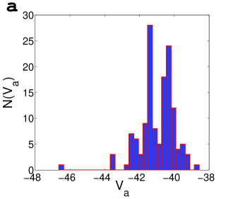
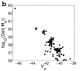
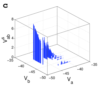
Figure 1: The essential PEL details, that go into the calculation of transition rates [Eq.(2)], are shown. Panel a: Histogram of IS energies. Panel b: Dependence of the overall curvature of a minimum on its energy. Panel c: Heights of the lowest energy barriers for going from minimum $a$ (with potential energy $V_{a}$) to minimum $b$ (with potential energy $V_{b}$).

II.3 Diffusion constant and waiting times

The diffusion constant $D$ can be calculated from the mean square displacement $\langle R^{2}(t)\rangle$ using $R_{ab}^{2}=N^{-1}\sum_{i=1}^{N}|\mathbf{r}_{i}^{(a)}-\mathbf{r}_{i}^{(b)}|^{2}$ in place of $\Phi_{ab}$ in Eq.(3) ($\mathbf{r}_{i}^{(a)}$ denotes the position of the $i$-th particle in the $a$-th minimum) and invoking the definition $D\equiv\lim_{t\rightarrow\infty}\frac{<R^{2}(t)>}{6t}=\lim_{t\rightarrow\infty}\frac{1}{6}\frac{d<R^{2}(t)>}{dt}$. This definition would yield $D=0$ here as $D=\lim_{t\rightarrow\infty}\sum_{a,b,n}\lambda_{n}(P^{0}_{a}P^{0}_{b})^{1/2}R_{ab}^{2}e_{a}^{(n)}e_{b}^{(n)}\exp{(-|\lambda_{n}|t)}=0$. In other words, $\langle R^{2}(t)\rangle\sim t^{\alpha(t)}$ and $\lim_{t\rightarrow\infty}\alpha(t)=0$. Instead, we can define the diffusive regime as the time window over which $\alpha(t)\simeq 1$ and then extract $D$ from the slope of the $\langle R^{2}(t)\rangle$ vs. $t$ plot in this region. This may not be useful for confined systems like the atomic cluster considered here, since such a diffusive regime may be very short or absent altogether, rendering $D$ to be an ill-defined quantity. Nevertheless, in this model we can define $D$ from the initial slope of the $\langle R^{2}(t)\rangle$ vs. $t$ curve as the usual ballistic regime ($\langle R^{2}(t)\rangle\propto t^{2}$), seen for instance at very short times in MD simulations, is absent by definition. So, we may define the diffusion constant as

$$D \equiv \lim_{t\rightarrow 0}\frac{d\langle R^{2}(t)\rangle}{dt}=\sum_{a,b}(P_{a}^{0}P_{b}^{0})^{1/2}R_{ab}^{2}\widetilde{W}_{ab}.$$ (9)

The waiting time in the basin of a minimum is the amount of time the system spends between an entry into and the subsequent exit from the basin (i.e. during a single visit to the basin). The average of this quantity for the $a$-th minimum, $\langle\tau_{w}(V_{a})\rangle$, can be calculated both from MD simulations and in the network model. In the master equation based model it is straightforward to write $\langle\tau_{w}(V_{a})\rangle$ as

$$\langle\tau_{w}(V_{a})\rangle \equiv \tau_{a}=-\frac{1}{W_{aa}}.$$ (10)

On the other hand, if we consider an ergodic MD trajectory, then the amount of time the system spends in $\mathcal{B}_{a}$ is $t_{a}\propto P_{a}^{0}$. Hence the total number of visits to $\mathcal{B}_{a}$ over the full trajectory can be written as $v_{a}\equiv(t_{a}/\tau_{a})\propto(P_{a}^{0}/\tau_{a})$. Finally, the mean waiting time averaged over the whole landscape would be

$$\tau_{w} = \frac{\sum_{a}\tau_{a}v_{a}}{\sum_{a}v_{a}}=-\frac{1}{\sum_{a}P_{a}^{0}W_{aa}}.$$ (11)

The above quantity can be related to $D$ [Eq.(9)] if $R_{ab}^{2}\simeq\bar{R}^{2}$ for all pairs of minima, as $D\simeq\bar{R}^{2}\sum_{a\neq b}(P_{a}^{0}P_{b}^{0})^{1/2}\widetilde{W}_{ab}=-\bar{R}^{2}\sum_{a}P_{a}^{0}W_{aa}=\bar{R}^{2}/\tau_{w}$. Hence for this special case the hopping between the basins becomes a random walk with a distribution of waiting times BDoliwa2 .

III Construction of the network for a 13-atom Morse cluster

The Morse potential PMMorse can be written in the form

$$V=\sum_{i<j}V_{ij},~{}~{}~{}~{}~{}V_{ij}=e^{\rho(1-r_{ij}/r_{e})}[e^{\rho(1-r_{ij}/r_{e})}-2]\epsilon,$$ (12)

where $r_{ij}$ is the distance between atoms $i$ and $j$, $\epsilon$ and $r_{e}$ are the dimer well depth and the equilibrium bond length, respectively - they simply scale the PEL without affecting its topology and can conveniently be set to unity and used as the units of energy and distance. The parameter $\rho$ is a dimensionless quantity that determines the range of the potential, with low values corresponding to long range. We have taken $\rho=4$. This potential is widely used to model inter-atomic interactions in small atomic clusters or molecules DJWales1 . The reduced unit of time can be set to $(mr_{e}^{2}/\epsilon)^{1/2}$, $m$ being the atomic mass.

We follow more-or-less the same procedure (described briefly in Appendix B) as that mentioned in Ref.MAMiller2 for building the network of minima and transition states. The network that we obtain consists of 138 minima and 230 transition states connecting them. We have not enforced any confining potential to prevent the cluster from melting - in the temperature range of our interest, the particles are confined due to interactions among themselves (we have discarded minima with maximum inter-particle separation more than 2.5). The minima and the transition states around a particular minimum are identified by the values of their potential energy.

In Fig.1 a, the distribution of inherent structure energies is shown. We index the inherent structures in ascending order of energy. The lowest lying minimum (the global minimum) is at $V_{a}=-46.635$ and after a substantial gap there are three minima at $V_{a}\simeq-43.5$; after that, another perceptible gap is present and the rest of the minima are closely spaced for $V_{a}\ {\raise-2.15277pt\hbox{$\buildrel>\over{\sim}$}}\ -42.5$. Henceforth, we denote by $\mathcal{N}_{f}$ the full network and by $\mathcal{N}_{r}$ the network with the four lowest-lying minima removed. When we remove a particular minimum, all its edges and minima that are connected to the rest of the network solely through this particular minimum get deducted from the network as well. As a result, $\mathcal{N}_{r}$ contains 52 minima and 70 transition states.

The overall curvature at a minimum, $\mathcal{C}$ is obtained from the determinant of the Hessian matrix at the minimum i.e. $\mathcal{C}=\mathrm{Det}(\mathbf{H})$. Here the deeper basins are narrower, as is evident from Fig.1 b. Also the number of barriers and barrier heights increase with decreasing IS energies (Fig.1 c).

In the next section we describe the results of the master equation based calculations carried out with the networks $\mathcal{N}_{f}$ and $\mathcal{N}_{r}$. While the relaxation dynamics in $\mathcal{N}_{f}$ is quite similar to that of strong glass formers, the dynamics in $\mathcal{N}_{r}$ shows strong resemblance to that of fragile ones. Although $\mathcal{N}_{r}$ is a part of $\mathcal{N}_{f}$, the relaxation of the system restricted in this part of the configuration space becomes qualitatively very different from the global dynamics in $\mathcal{N}_{f}$.

The procedure of searching for transition states (Appendix B) starting at a minimum and moving along directions of successively larger eigenvalues of the Hessian matrix is not very efficient TFMiddleton and most of the time, one ends up at the same transition state. Hence we get only 3 barriers around a minimum on the average. Although the details of the connectivity of the network may matter for finer details, our main objective in this work has been to realize the typical characteristics of glassy dynamics with a minimal set of minima and transition states. Hence we have not paid much attention to building the network very accurately so as to represent the actual system. Nevertheless, the network model seems to capture the main features of the complex long-time dynamics quite accurately, as verified through MD simulations (Section V).

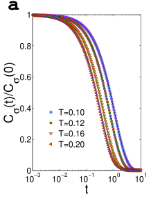
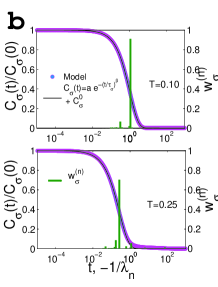
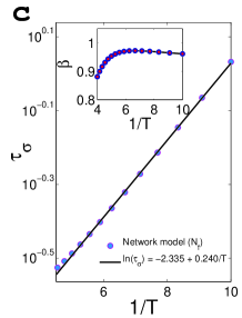
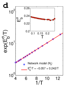
Figure 2: Stress autocorrelation function for the network $\mathcal{N}_{f}$ (Section III). Panel a: $C_{\sigma}(t)$ [normalized by dividing with $C_{\sigma}(0)$] is shown for various $T$. Panel b: Decay of $C_{\sigma}(t)$ is determined by one dominant relaxation mode $n$ over the entire temperature range of interest, as is evident from the plot of $w_{\sigma}^{(n)}$ vs. $|\lambda_{n}|^{-1}$ [Eq.(7)] for $T=0.10,~{}0.25$. Panel c: Arrhenius plot for $\tau_{\sigma}(T)$ [extracted by fitting $C_{\sigma}(t)$ with the KWW form of Eq.(5)] i.e. $\ln\tau_{\sigma}$ vs. $1/T$. The effective barrier $E_{b}^{\sigma}$ is obtained by fitting the data to the Arrhenius form [Eq.(13)]. The stretching exponent $\beta\simeq 1$ (inset) confirms the simple exponential nature of the decay. Panel d: The estimate of Eq.(16a) (Appendix A) for $E_{b}^{\sigma}$ agrees very well with the value of $E_{b}^{\sigma}=0.24$ obtained from the Arrhenius fit shown in panel c.

IV Strong and fragile behavior in the network model

Here we describe the results for the stress-stress autocorrelation function $C_{\sigma}(t)$, as described in Sec.II.2, for the Morse cluster.

Fig.2 a shows $C_{\sigma}(t)$ for the network $\mathcal{N}_{f}$ at four different temperatures. The decay of the correlation function is very well described by a single exponential [the stretching exponent of Eq.(5), $\beta\simeq 1$] over the entire temperature range, as is evident from the inset of Fig.2 c. The origin of this simple Debye-like relaxation can be attributed to the presence of a single relaxation mode with a large weight $w_{\sigma}^{(n)}$ [Eq.(7)] as shown in Fig.2 b. The corresponding relaxation time $\tau_{\sigma}$ extracted by fitting $C_{\sigma}(t)$ with Eq.(5) follows an Arrhenius temperature dependence (Fig.2 c), i.e.

$$\tau_{\sigma}=\tau_{\sigma}^{0}\exp{\left(\frac{E_{b}}{T}\right)}$$ (13)

In $\mathcal{N}_{f}$, the dynamics is mainly governed by the barriers connecting the global minima at $V_{a}\simeq-46.6$ with the next three lowest lying minima at $V_{a}\simeq-43.5$ (see Section III).

The Arrhenius fit to $\tau_{\sigma}$ vs. $T$ curve yields an effective activation barrier $E_{b}^{\sigma}=0.24$ which one can easily identify with the barrier for going from one of the minima at $V_{a}\simeq-43.5$ to the global minimum. The estimate for $E_{b}^{\sigma}$ (Fig.2 d) obtained from Eq.(16a) (Appendix A) agrees very well with the above value. In contrast, we find that the barrier for going from the global minimum to the next lowest lying minimum determines the effective activation barrier that appears in the $T$-dependence of the mean waiting time $\tau_{w}$ [Eq.(11)]. This is a natural consequence of the fact that the global minimum, being much lower in potential energy with respect to the other minima in this case, possesses almost all the Boltzmann weight. As a result, the relaxation to equilibrium (decay of correlation) is entirely dictated by the relaxation paths from other parts of the PEL to the global minimum. The mean waiting time $\tau_{w}$, on the other hand, is decided by the escapes from the global minimum over the barriers surrounding it as the system spends most of the time in the basin of the global minimum.

The above observations suggest a trivial route for realizing strong behavior, namely dynamics governed by a fixed set of barriers surrounding a very deep inherent structure (or a set of inherent structures with very similar potential energies in a more general case) possessing most of the Boltzmann occupation probability. Keeping this fact in mind we construct the network $\mathcal{N}_{r}$ by removing a few deep minima so that a larger number of minima figure in the relaxation to equilibrium due to comparable Boltzmann weights in the activated regime and many different barriers contribute to the relaxation process.

Fig.3 a exhibits $C_{\sigma}(t)$ calculated for $\mathcal{N}_{r}$. We observe a two-stage, non-exponential relaxation in this case. This, again, can be understood from the values of $w_{\sigma}^{(n)}$ (Fig.3 b). The profile of $C_{\sigma}(t)$ is well fitted with a sum of two stretched exponentials, i.e. $C_{\sigma}(t)=C_{\sigma}^{(1)}(t)+C_{\sigma}^{(2)}(t)=C_{\sigma}^{(1)}(0)e^{-(t/\tau_{\sigma}^{(1)})^{\beta_{1}}}+C_{\sigma}^{(2)}(0)e^{-(t/\tau_{\sigma}^{(2)})^{\beta_{2}}}$. We plot the longer of the two relaxation times, $\tau_{\sigma}^{(2)}$, in Fig.3 c along with the exponent $\beta_{2}$ in the inset. The deviation from simple exponential behavior is evident. The temperature dependence of $\tau_{\sigma}^{(2)}$ exhibits marked deviation from the simple Arrhenius behavior. Rather, the Vogel-Fulcher-Tammann (VFT) form HVogel ; GSFulcher ; GTammann ,

$$\tau_{\sigma}=\tau_{\sigma}^{0}\exp{\left(\frac{B_{\sigma}}{T-T_{0}^{\sigma}}\right)},$$ (14)

frequently used for fragile glass formers, yields a much better representation of the data for $\tau_{\sigma}^{(2)}$. The fragile nature of the $\ln\tau_{\sigma}^{(2)}$ vs. $1/T$ curve is well reproduced in Fig.3 d by the effective temperature dependent barrier $E_{b}^{\sigma}(T)$ calculated from Eq.(16a).

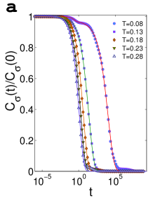
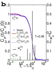
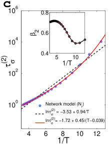
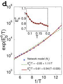
Figure 3: Stress autocorrelation function in $\mathcal{N}_{r}$. Panel a: $C_{\sigma}(t)$ is shown for five $T$ values. Panel b: Fit to a sum of two stretched exponentials (Eq.(5), see the text for details) at $T=0.08$. The quantity $w_{\sigma}^{(n)}$ exhibits the presence of (well-separated) multiple timescales even at the very low temperature $T=0.08$. Panel c: The deviation from the simple Arrhenius form is evident from the plot of $\ln\tau_{\sigma}^{(2)}$ vs. $1/T$. Fits to both the Arrhenius form [Eq.(13)] and the VFT form [Eq.(14)] are shown. It is clear that the VFT form provides a good fit. Inset: The exponent $\beta_{2}$ is much less than 1, specially at low temperatures, showing the non-exponential nature of the relaxation. Panel d, The effective barrier $E_{b}^{\sigma}(T)$ obtained from Eq.(16a) agrees reasonably well with the estimate deduced from the Arrhenius and VFT fits. For instance, the VFT fit to $\exp{(E_{b}^{\sigma}/T)}$ vs. $1/T$ yields values for the parameters $B_{\sigma}$ and $T_{0}^{\sigma}$ [Eq.(14)] that are similar to those obtained in panel c.

A useful visualization and understanding of the observed strong behavior for the PEL $\mathcal{N}_{f}$ and fragile behavior for $\mathcal{N}_{r}$ can be achieved by looking at the quantity $\mathcal{W}_{ab}$ defined in Eq.(16b) and the subsequent paragraph of Appendix A. This quantity, $\mathcal{W}_{ab}$, can be thought of as the weight with which the edges between the nodes $a$ and $b$, or in other words, the elementary jumps over the barriers connecting minima $a$ and $b$ appears in the relaxation process through various relaxation channels or modes $n$. In Figs.4 a, b and c we have shown the color maps of $\mathcal{W}_{ab}$ for $\mathcal{N}_{f}$ at three temperatures. In these plots, the coordinates $(V_{a},V_{b})$ represent the barrier between minima $a$ and $b$ and the color corresponds to the value of $\mathcal{W}_{ab}$ at $(V_{a},V_{b})$ (we have used a small broadening for the purpose of visualization). It is clear from the plots that only a few barriers surrounding the global minimum contribute substantially to the relaxation process and over the entire temperature range, the peaks remain at nearly the same positions. On the contrary for $\mathcal{N}_{r}$, in Figs. 4 d, e and f, many barriers figure in the activated relaxation and the picture changes substantially with increasing temperature, as more and more barriers start to play a role in the relaxation process. This feature can be considered as the trademark of fragile dynamics.

We have observed similar characteristics of strong and fragile dynamics for the relaxation time $\tau_{\delta}$ associated with the overlap function $C_{\delta}(t)$, defined in Section II.2, obtained from both the network model calculation and MD simulations. We report these results in the next section.

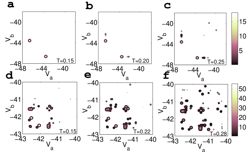
Figure 4: Color maps (see the color bars) for $\mathcal{W}_{ab}$ [Eq.(16b)] in the $(V_{a},V_{b})$ plane for $\mathcal{N}_{f}$ at three temperatures, $T=0.15$ (panel a), $T=0.20$ (panel b), and $T=0.25$ (panel c), and for $\mathcal{N}_{r}$ at $T=0.15$ (panel d), $T=0.22$ (panel e), and $T=0.28$ (panel f).

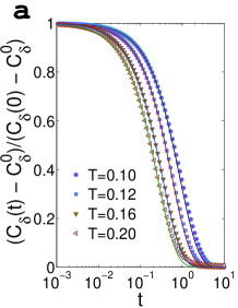
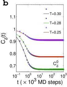
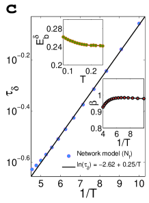
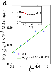
Figure 5: Overlap function $C_{\delta}(t)$ for the network $\mathcal{N}_{f}$. Panel a: $(C_{\delta}(t)-C_{\delta}^{0})/(C_{\delta}(0)-C_{\delta}^{0})$ obtained from the network model for four temperatures. Panel b: MD results for $C_{\delta}(t)$. Panel c: Arrhenius plot for $\tau_{\delta}(T)$ deduced in a from KWW fits [Eq.(5)]. The top and bottom insets show, respectively, the estimates of $E_{b}^{\delta}(T)$ from Eq.(16a) and the stretching exponent $\beta$ for the KWW fit to $C_{\delta}(t)$ in a. Panel d: Estimates of $\tau_{\delta}$ can be obtained accurately only for a narrow temperature range in MD, as discussed in the text. The exponent $\beta$, extracted from b, is shown in the inset.

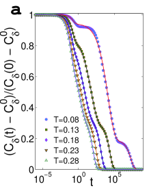
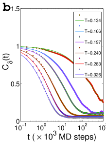
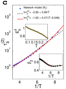
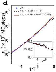
Figure 6: Overlap function $C_{\delta}(t)$ for the network $\mathcal{N}_{r}$. Panel a: $C_{\delta}(t)$ calculated in the network model exhibits multi-step decay of correlation. Panel b: $C_{\delta}(t)$ as obtained by confining the MD trajectory in a part of the configuration space that excludes the basins of attraction of the first four lowest-lying inherent structures. Panel c: The intermediate relaxation time $\tau_{\delta}^{(2)}$ obtained by fitting the data for $C_{\delta}(t)$ in a with the sum of three stretched exponentials. Here the $\ln\tau_{\delta}^{(2)}$ vs. $1/T$ plot shows a small bending indicating deviations from the Arrhenius $T$-dependence. The VFT fit is also shown. the upper and lower insets show, respectively, the $E_{b}^{\delta}(T)$ calculated from Eq.(16a) and the exponent $\beta_{2}$ from the fits to $C_{\delta}(t)$ at different temperatures. d, The results for $\tau_{\delta}(T)$ obtained in MD simulations agree with the fragile behavior observed in the network model. The semiquantitative agreement can be verified by comparing the VFT fits for $\tau_{\delta}(T)$ in the network model and in MD.

V Comparison of the results of the network model with those of MD

We have carried out MD simulations DFrenkel for the cluster of 13 particles interacting via the Morse potential [Eq.(12)]. Initial long MD runs along with regular quenching provide the starting data base of minima and then we follow the procedure of Appendix B to improve the list as well as to construct the network of minima and transition states. The main motivation of our MD study is to check to what extent the dynamics of the systems is captured by the network model by comparing the results of the network model calculation with those for the real dynamics (i.e. Newton’s equation of motion). We find that the main results of the network model calculation are supported both qualitatively and quantitatively by the MD results. As already discussed in the introduction, the model assumes that there is a clear separation between the time scales of local vibrations and activated jumps. This assumption is bound to be valid at very low temperature where the barriers are much higher than the temperature. However, the barrier heights have a wide distribution (Fig.1 c) and hence the assumption of well separated time scales may be invalidated at different temperatures for different parts of the landscape. Presumably, as the temperature is increased, the dynamics crosses over from a landscape dominated regime at low temperatures to a high-temperature regime where the system does not see the details of the PEL due to its large thermal energy and the dynamics is no longer dominated by activation processes.

We have calculated the stress autocorrelation function $C_{\sigma}(t)$ and the overlap function $C_{\delta}(t)$ (Sec.II.2) from MD simulations at different temperatures. Also, we have estimated the mean waiting times and waiting time distributions. We find that due to intra-basin relaxation present in MD, the stress autocorrelation function $C_{\sigma}(t)$ decays within the vibrational time periods of the local minima much before the inter-basin jump dynamics comes into play. As a result, $C_{\sigma}(t)$ is not useful for comparison with the network model results. Hence we concentrate on $C_{\delta}(t)$ and the related relaxation time since by definition the decay of $C_{\delta}(t)$ is entirely determined by inter-basin transitions. For calculating this quantity as well as the waiting times for different minima, we construct a discontinuous trajectory in terms of configurations of inherent structures from the MD trajectory and track the transitions along it by the interval bisection method described in reference BDoliwa1 [see Appendix C].

For comparing the results obtained for $\mathcal{N}_{r}$ (Sec.III), additionally, we need to confine the MD trajectories in a restricted part of the configuration space so that the basins of the four lowest-lying minima are not visited (see Appendix C). This goal is achieved by applying a procedure similar to that described in Refs SFChekmarev1 ; SFChekmarev2 . The application of this method in conjunction with the interval bisection method makes the MD runs very time consuming and hence it is difficult to get very long MD trajectories (typically $10^{8}$ or $10^{9}$ MD steps with the MD step length $\delta t=0.001$). So we have averaged over many parallel runs with smaller number of MD steps ($2\times 10^{7}$ for $\mathcal{N}_{f}$ and $2\times 10^{6}$ to $2\times 10^{7}$ for $\mathcal{N}_{r}$, depending on the temperature) starting from different parts of the landscape i.e. different initial conditions (different IS configurations are taken from the already existing data base).

We compare the results for $C_{\delta}(t)$ obtained through the network model for $\mathcal{N}_{f}$ and $\mathcal{N}_{r}$ with those obtained via isokinetic MD DFrenkel in Figs.5 and 6, respectively. Fig.5 a shows the network model results for $C_{\delta}$ in $\mathcal{N}_{f}$. Corresponding MD results are shown in Fig.5 b. The Arrhenius plots for associated relaxation times are shown in Figs.5 c and d. The strong behavior is evident and decays of $C_{\delta}(t)$ in both the cases are close to exponential ($\beta\simeq 0.9$) as exhibited in the insets of these figure panels. A good estimate of the effective activation energy is once again obtained from Eq.(16a) (inset of Fig.5 c). Here the effective barrier $E_{b}^{\delta}\simeq 0.25$ is comparable to $T$ in the temperature range of interest and hence the associated time scale for relaxation is quite short. Even then, an accurate calculation of the correlation function $C_{\delta}(t)$ and the relaxation time $\tau_{\delta}$ in MD is quite difficult because the system gets trapped in the deep global minimum most of the time and a proper sampling of the relevant relaxation paths connecting the higher minima to the global one becomes hugely time consuming and increasingly difficult with decreasing temperature. As a result we can estimate $\tau_{\delta}$ only for a limited range of temperatures, as shown in Fig.5d. Also for temperatures higher than $T\simeq E_{b}^{\delta}\simeq 0.25$ the network model dealing only with the activated processes becomes unreliable, rendering a comparison with MD results inappropriate.

For the network $\mathcal{N}_{r}$, $C_{\delta}(t)$ exhibits a three-stage relaxation profile (Fig.6 a) owing to the presence of well-separated time scales similar to the case of $C_{\sigma}(t)$ (Fig.3 b). Such a clear cut separation of timescale is not observed in the corresponding microcanonical MD DFrenkel results for $C_{\delta}(t)$ shown in Fig.6 b, although a faint signature of multi-step relaxation can be seen at low temperatures. The decays of $C_{\delta}(t)$ at various temperatures, shown in Fig.6 a, are fitted to a sum of three stretched exponentials [Eq.(5)]. The temperature dependence of the intermediate relaxation time $\tau_{\delta}^{(2)}(T)$ shows deviations from the Arrhenius form [Eq.(13)] in Fig.6 c, although much less in extent than that for $\tau_{\sigma}^{(2)}(T)$ (Fig.3 c). The latter fact is indicative of the importance of the quantity $\Phi_{ab}$ of Eq.(3), i.e. the quantity whose autocorrelation function is used to calculate the relaxation time, in determining the degree of fragility obtained from the temperature dependence of the relaxation time. As discussed above, the distribution and temperature dependence of the quantities $\mathcal{W}_{ab}^{\phi}$, which depend on the quantity $\phi({\bf r})$ whose autocorrelation function is used to calculate the relaxation time (see Appendix A), play an important role in determining the degree of fragility. We have checked that plots of $\mathcal{W}_{ab}$ for the overlap function, similar to those shown in Fig. 4, exhibit a less pronounced dependence on the temperature. This is consistent with the observation that the temperature dependence of the relaxation time extracted from the decay of the overlap function exhibits smaller deviations from the Arrhenius form (lower degree of fragility) in comparison to that for the relaxation time obtained from the stress autocorrelation function. The Arrhenius fit parameter $E_{b}^{\delta}$ and VFT fit parameters $B_{\delta}$ and $T_{0}^{\delta}$ are shown in Fig.6 c. These agrees reasonably well with the results of similar fits done for $\tau_{\delta}$ estimated through MD simulations (Fig.6 d).

VI Conclusion

Our work shows that the master equation based approach, first proposed by Angelani et al.LAngelani1 , for the landscape dominated activated dynamics on a network of minima and transition states is capable of addressing many important issues and challenges related to glassy dynamics. Our results for the full network $\mathcal{N}_{f}$ are similar to those of Refs.LAngelani1 ; LAngelani2 where strong behavior in the dynamics, arising from the dominance of the global minimum and the barriers surrounding it, was observed. Our study of the restricted network $\mathcal{N}_{r}$ leads to the important result that the master equation approach may lead to fragile dynamic behavior if many inherent structures and the barriers between pairs of them are involved in the relaxation process. This conclusion is confirmed by our MD simulations. Our study, thus, provides valuable insights into the origin of fragile dynamic behavior in glass-forming liquids. It also illustrates the usefulness of the master equation approach in studies of glassy dynamics. Due to computational constraints, the applicability of this approach has been limited to small system sizes till now. A related approach AKushima that differs from the one considered here in the details of its implementation seems to be a promising one for studying larger systems. Another interesting future direction for studying moderately large systems might be to extend this framework for the dynamics in the metabasin space to obtain quantities relevant for the characterization of glassy dynamics.

Acknowledgements

We thank Smarajit Karmakar, Pinaki Chaudhury and Biswaroop Mukherjee for useful discussions. SB would like to acknowledge CSIR (Government of India) and DST (Govt. of India) for support. CD acknowledges support from DST(Govt. of India).

Appendix A Effective activation energy

As mentioned in Section II.1, $\tau_{n}=|\lambda_{n}|^{-1}$ is the relaxation time corresponding to the $n$-th mode ($n\geq 2$) and $w_{\phi}^{(n)}$ [Eq.(7)] provides the distribution of such relaxation times. We assume that the relaxation time for each individual mode is governed by an effective barrier $E_{b}^{(n)}$ i.e. $\tau_{n}\propto\exp{(E_{b}^{(n)}/T)}$. Hence we can estimate $E_{b}^{(n)}$ approximately from the local slope of the $\ln\tau_{n}$ vs. $1/T$ curve as follows

$$E_{b}^{(n)}\simeq-\frac{1}{\lambda_{n}}\frac{\partial|\lambda_{n}|}{\partial(1/T)}$$

$$\simeq\frac{1}{|\lambda_{n}|}\sum_{<ab>,s}\left[(V_{ab}^{s}-V_{a})(\mathcal{U}_{s,a}^{(n)})^{2}+(V_{ab}^{s}-V_{b})(\mathcal{U}_{s,b}^{(n)})^{2}\right.$$

$$\left.-2(V_{ab}^{s}-\frac{V_{a}+V_{b}}{2})\mathcal{U}_{s,a}^{(n)}\mathcal{U}_{s,b}^{(n)}\right]$$ (15a)

with

$$\mathcal{U}_{s,a}^{(n)} = (\Lambda_{ab}^{s})^{1/2}\left[\frac{\mathrm{Det}(\mathbf{H}_{a})}{\mathrm{Det}(\mathbf{H}_{ab}^{s})}\right]^{1/4}e^{-\frac{V_{ab}^{s}-V_{a}}{2T}}e_{a}^{(n)}$$ (15b)

To obtain the expression (15a) for $E_{b}^{(n)}$ we have rewritten $\lambda_{n}$ as $\sum_{a,b}\widetilde{W}_{ab}e_{a}^{(n)}e_{b}^{(n)}$ and while taking the derivative of $\lambda_{n}$ with respect to $T$ neglected the temperature dependence of the eigenvector $\mathbf{e}^{(n)}$ assuming it to be weakly temperature dependent. We find this to be valid for the case of the 13-atom Morse cluster and the above approximation for $E_{b}^{(n)}$ seems to work, as we have reported in Sections IV and V. The overall effective activation energy $E_{b}^{\phi}(T)$ is obtained by summing over the contributions of all the modes appearing with the weights $w_{\phi}^{(n)}$ [Eq.(7)], i.e. $E_{b}^{\phi}\equiv\sum_{n\geq 2}E_{b}^{(n)}w_{\phi}^{(n)}$. This can be recast as

$$E_{b}^{\phi} = \sum_{<ab>}\mathcal{W}_{<ab>}^{\phi}E_{<ab>}^{\phi}$$ (16a)

here,

$$\mathcal{W}_{<ab>}^{\phi} \equiv \sum_{s}\mathcal{W}_{s,<ab>}^{\phi}$$ (16b)

$$E_{<ab>}^{\phi} \equiv \frac{\sum_{s}\mathcal{E}_{s,<ab>}^{\phi}}{\sum_{s}\mathcal{W}_{s,<ab>}^{\phi}}$$ (16c)

with

$$\mathcal{W}_{s,<ab>}^{\phi}=\sum_{n\geq 2}|\lambda_{n}|^{-1}w_{\phi}^{(n)}(\mathcal{U}_{s,a}^{(n)}-\mathcal{U}_{s,b}^{(n)})^{2}$$

$$\mathcal{E}_{s,<ab>}=\sum_{n\geq 2}|\lambda_{n}|^{-1}w_{\phi}^{(n)}\left[V_{ab}^{s}(\mathcal{U}_{s,a}^{(n)}-\mathcal{U}_{s,b}^{(n)})^{2}\right.$$

$$\left.-(V_{a}\mathcal{U}_{s,a}^{(n)}-V_{b}\mathcal{U}_{s,b}^{(n)})(\mathcal{U}_{s,a}^{(n)}-\mathcal{U}_{s,b}^{(n)})\right]$$

The effective barrier $E_{b}^{\phi}(T)$ obtained from Eq.(16a) compares quite well with the barrier extracted from the $T$-dependence of the relaxation time $\tau_{\phi}$ estimated by fitting the KWW form [Eq.(5)] to the correlation function $C_{\phi}(t)$, computed using Eq.(3) for the Morse cluster. The quantity $\mathcal{W}_{ab}^{\phi}=\mathcal{W}_{ba}^{\phi}\equiv\mathcal{W}_{<ab>}^{\phi}/2$ can be a good measure of the relative importance of a pair of minima or an elementary jump in the relaxation process as demonstrated in Section IV.

Appendix B Construction of the network of minima and transition states

As mentioned in Sec.III, we follow the procedure similar to that in Ref. MAMiller2 for building the network model for the 13-atom Morse cluster. We have used the OPTIM package Optim , developed by D. J. Wales and co-workers, to search for minima and transition states as follows

1. Do long MD simulations and steepest descent quenches in regular intervals to reach nearby minima along the MD trajectories. Distinction between configurations of minima is done in terms of their potential energy values. This provides us with an initial data base or list of minima.

2. Starting from each of these minima, one by one,

   1. search for a transition state along the eigenvector with the lowest eigenvalue.

   2. After reaching a transition state, do steepest descent minimization starting parallel to the transition vector, i.e. eigenvector corresponding to the negative eigenvalue, at the transition state to arrive at the minima connected directly to initial one (sometimes, following the eigenvector from a minimum we obtain states which are not connected to it by steepest descent - we discard these states). This establishes one edge, constituted of a pair of minima connected by a transition state, of the network.

   3. Repeat (a) beginning anti-parallel to the eigenvector with the lowest eigenvalue and then successively in both directions along eigenvectors with ascending eigenvalues until all the eigendirections are considered at the starting minimum.

   4. If some new minima, not in the starting list, are found in this process we append them to the data base and modify the existing list of minima.

3. Repeat 2 until all the minima in the data base are searched.

Appendix C Interval bisection and confinement of MD trajectories in a specified part of the PEL

Starting from a MD trajectory, $\mathbf{r}(t)=(\mathbf{r}_{1}(t),\mathbf{r}_{2}(t),...,\mathbf{r}_{N}(t))$, we construct a trajectory $\mathbf{r}^{0}(t)=(\mathbf{r}_{1}^{0}(t),\mathbf{r}_{2}^{0}(t),...,\mathbf{r}_{N}^{0}(t))$ in terms of the inherent structure configurations by doing steepest descent minimization at regular intervals BDoliwa1 . The straightforward way, though computationally impractical, is to do minimization at every time step. Also there may be many back and forth jumps between neighboring minima giving rise to events that do not affect the long time relaxation which we are mainly interested in. Bearing this fact in mind, we do quenches for equidistant points, $t_{n}=n\Delta t$ ($n$ being an integer) to get $\mathbf{r}^{0}(t_{n})$ with $\Delta t=100-200$ MD steps (around $1/10$-th of the typical vibrational period at a minimum for the Morse cluster). During a MD run, starting from initial point ($n=0$),

1. Save the trajectory $\mathbf{r}(t)$ between $t_{i}=t_{n}$ and $t_{f}=t_{n+1}$ and then follow the steps described below provided $\mathbf{r}^{0}(t_{i})\neq\mathbf{r}^{0}(t_{f})$ (actually we compare $V(\mathbf{r}^{0})$ instead of $\mathbf{r}^{0}$),

   1. Set $t_{m}=(t_{i}+t_{f})/2$ and get $\mathbf{r}^{0}(t_{m})$ from $\mathbf{r}(t_{m})$.

   2. If $\mathbf{r}^{0}(t_{m})=\mathbf{r}^{0}(t_{i})$, set $t_{i}=t_{m}$ else set $t_{f}=t_{m}$.

   3. Go on repeating steps (a) and (b) until $t_{f}-t_{i}=1$.

2. Change $n$ to $n+1$ and go back to 1.

Next we describe the method that we have adopted for restricting the trajectory of the state point of the system to a part of the configuration space. This is an extension of the interval bisection method described in the preceding paragraph. The trajectory is constructed part by part successively and in each part, whenever we detect a transition (using the interval bisection method) from the allowed part to forbidden part (say the part containing the basins of attraction of the four lowest-lying minima with $V_{a}<-43$ in the case of the 13-atom Morse cluster), we re-initiate the MD at the point when the system last visited the allowed part using new velocities for the particles. We assign random velocities drawn from a Maxwell distribution at temperature $T$ [in the case of microcanonical simulation at constant $E_{\mathrm{tot}}$, the temperature is obtained from the total kinetic energy at the instant when the system last visited the allowed part i.e. $T=2(E_{\mathrm{tot}}-V)/(3N-6)$]. After each such re-initiation we correct for the integrals of motion i.e. energy, momentum and angular momentum by suitable rescaling and rotation of the velocities.

Under this procedure the dynamics no longer remains truly Newtonian due to repeated velocity re-initiations. We have calculated the velocity autocorrelation function which decays very fast (within 2000 MD steps i.e. $\sim$1-2 vibrational periods) and heuristically we can argue that successive velocity re-initiations are more or less uncorrelated. Nonetheless, following reference SFChekmarev2 we have performed a few standard checks by computing quantities that can be accessed through the above mentioned confined MD as well as through the regular unrestricted MD procedure and we found good agreement between the results obtained in these two different ways. For instance, the distributions of the total kinetic energy and the waiting time for a restricted part of the configuration space (e.g. the basin of attraction of a particular minimum) can be estimated SFChekmarev2 both by enforcing the trajectory to sample only the specified part or by picking out from a conventional long MD trajectory the intervals during which the system samples the specified part.

We find that there are some spurious effects in the dynamics due to cycling of trajectories near the saddles or the system spending more time near the border of the allowed and forbidden regions. Also, at low temperatures, when the system is constrained in the high energy parts such as $\mathcal{N}_{r}$, it has a tendency to visit the lowest lying basins more often. In the above mentioned procedure the system can visit the forbidden region within the small interval $\Delta t$ and come back to the allowed part. We find these events to affect the properties related to short time relaxation such as the diffusion constant [Eq.(9)], waiting time $\tau_{w}$ [Eq.(11)] and its distribution. While restricting the system in $\mathcal{N}_{r}$, as the system frequently escapes to the four lower lying basins, the barrier that appears in the temperature dependence of $D$ and $\tau_{w}$ turns out to be related to the barriers connecting $\mathcal{N}_{r}$ to the forbidden low-energy part. However, since these visits are really short lived ($\leq 100-200$ MD steps), they do not affect the features of long-time relaxation, such as the decay of correlations characterized by $C_{\delta}(t)$.

References

- (1) C. A. Angell, J. Phys.: Condens. Matter 12, 6463 (2000).
- (2) See the article by W. Kob in Slow Relaxations and Nonequilibrium Dynamics in Condensed Matter, edited by J.-L. Barrat, M. Feigelman, and J. Dalibard (Springer, Berlin, 2003).
- (3) P. G. Debenedetti and F. H. Stillinger, Nature 419, 259 (2001).
- (4) C. A. Angell, P. H. Poole and J. Shao, Nuovo Cimento D 16, 993 (1994).
- (5) G. Ruocco, F. Sciortino, F. Zamponi, C. De Michele and T. Scopigno, J. Chem. Phys. 120, 10666 (2004).
- (6) M. Goldstein, J. Chem. Phys. 51, 3728 (1969).
- (7) D. J. Wales, Energy Landscapes (Cambridge University Press, Cambridge, 2003).
- (8) K. Binder and A. P. Young, Rev. Mod. Phys. 58, 801 (1986).
- (9) F. H. Stillinger and T. A. Weber, Phys. Rev. A 25, 978 (1982).
- (10) F. H. Stillinger and T. A. Weber, Phys. Rev. A 28, 2408 (1983).
- (11) F. H. Stillinger, Science 267, 1935 (1995).
- (12) F. H. Stillinger, J. Chem. Phys. 88, 7818 (1988).
- (13) S. Sastry, P. G. Debenedetti and F. H. Stillinger, Nature 393, 554 (1998).
- (14) D. Frenkel and B. Smit, Understanding Molecular Simulation (Academic Press, San Diego, 1996).
- (15) L. Angelani, G. Parisi, G. Ruocco and G. Viliani, Phys. Rev. Lett. 81, 4648 (1998).
- (16) L. Angelani, G. Parisi, G. Ruocco and G. Viliani, Phys. Rev. E 61, 1681 (2000).
- (17) M. A. Miller, J. P. K. Doye and D. J. Wales, Phys. Rev. E 60, 3701 (1999).
- (18) F. H. Stillinger, Phys. Rev. E 59, 48 (1999).
- (19) B. Doliwa and A. Heuer, Phys. Rev. E 67, 031506 (2003).
- (20) A. Heuer, J. Phys.:Condens. Matter 20, 373101 (2008).
- (21) Y. Yang and B. Chakraborty, Phys. Rev. E 80, 011501 (2009).
- (22) T. F. Middleton and D. J. Wales, Phys. Rev. B 64, 024205 (1999).
- (23) J. P. K. Doye and C. P. Massen, J. Chem. Phys. 122, 084105 (2005).
- (24) P. M. Morse, Phys. Rev. 34, 57 (1929).
- (25) M. A. Miller, J. P. K. Doye and D. J. Wales, J. Chem. Phys. 110, 328 (1999).
- (26) S. F. Chekmarev, Phys. Rev. E 64, 036703 (2001).
- (27) S. F. Chekmarev and S. V. Krivov, Chem. Phys. Lett. 287, 719 (1998).
- (28) W. H. Press, S. A. Teukolsky, W. T. Vetterling and B. P. Flannery, Numerical Recipes in C (Cambridge University Press, Cambridge, 1992).
- (29) C. J. Cerjan and W. H. Miller, J. Chem. Phys. 75, 2800 (1981).
- (30) http://www-wales.ch.cam.ac.uk/software.html.
- (31) H. A. Kramers, Physica 7, 284 (1940).
- (32) J. S. Langer, Ann. Phys. 54, 258 (1969).
- (33) P. Hnggi, P. Talkner and M. Borkovec, Rev. Mod. Phys. 62, 251 (1990).
- (34) R. Kohlrausch, Ann. Phys. (Leipzig) 12, 393 (1847).
- (35) G. Williams and D. C. Watts, Trans. Faraday Soc. 66, 80 (1980).
- (36) J. P. Hansen and I. R. McDonald, Theory of Simple Liquids (Academic Press, San Diego, 1976).
- (37) B. Doliwa and A. Heuer, Phys. Rev. E 67, 030501 (2003).
- (38) H. Vogel, Phys. Z. 22, 645 (1921)
- (39) G. S. Fulcher, J. Amer. Ceram. Soc. 8, 339 (1925).
- (40) G. Tammann and W. Z. Hesse, Anorg. Allg. Chem. 156, 245 (1926).
- (41) A. Kushima et al., J. Chem. Phys. 130, 224504 (2009).