Superfield approach to nilpotent symmetries in 3D Jackiw-Pi
model of massive non-Abelian theory

S. Gupta^(a), R. Kumar^(a), R. P. Malik^(a,b)
(a) Physics Department, Centre of Advanced Studies,
Banaras Hindu University, Varanasi - 221 005, (U.P.), India

and

^(b) DST Centre for Interdisciplinary Mathematical Sciences,
Faculty of Science, Banaras Hindu University, Varanasi - 221 005, India
E-mails: saurabh@imsc.res.in; raviphynuc@gmail.com; rpmalik1995@gmail.com

Abstract: In the available literature, only the Becchi-Rouet-Stora-Tyutin (BRST) symmetries are known for the Jackiw-Pi model of the three (2 + 1)-dimensional (3D) massive non-Abelian gauge theory. We derive the off-shell nilpotent $(s_{(a)b}^{2}=0)$ and absolutely anticommuting $(s_{b}\,s_{ab}+s_{ab}\,s_{b}=0)$ (anti-)BRST transformations $s_{(a)b}$ corresponding to the usual Yang-Mills gauge transformations of this model by exploiting the “augmented” superfield formalism where the horizontality condition and gauge invariant restrictions blend together in a meaningful manner. There is a non-Yang-Mills (NYM) symmetry in this theory, too. However, we do not touch the NYM symmetry in our present endeavor. This superfield formalism leads to the derivation of an (anti-)BRST invariant Curci-Ferrari restriction which plays a key role in the proof of absolute anticommutativity of $s_{(a)b}$. The derivation of the proper anti-BRST symmetry transformations is important from the point of view of geometrical objects called gerbes. A novel feature of our present investigation is the derivation of the (anti-)BRST transformations for the auxiliary field $\rho$ from our superfield formalism which is neither generated by the (anti-)BRST charges nor obtained from the requirements of nilpotency and (or) absolute anticommutativity of the (anti-)BRST symmetries for our present 3D non-Abelian 1-form gauge theory.

PACS numbers: 11.15.-q; 03.70.+k; 11.10.Kk; 12.90.+b

Keywords: Jackiw-Pi model; 3D massive gauge theory; superfield formalism; (anti-)BRST symmetries; nilpotency and absolute anticommutativity; Curci-Ferrari condition

1 Introduction

The 4D (non-)Abelian 1-form gauge theories are at the heart of standard model of particle physics where there is a stunning degree of agreement between theory and experiment. One of the weak links of SM is connected with the very existence of the Higgs particle, which is responsible for the mass generation of gauge bosons and fermions. In view of the fact that Higgs particle has not yet been observed experimentally with a hundred percent certainty, other theoretical tools for the mass generation of gauge bosons (in various dimensions of space-time) have become important and they have generated a renewed interest in the realm of theoretical physics. From many angles, the mass generation in gauge theory is an important issue.

In the above context, it may be mentioned that the 4D topologically massive (non-) Abelian gauge theories have been studied in the past [1, 2, 3, 4] where there is merging and mixing of 1-form and 2-form (non-)Abelian gauge fields through the celebrated topological $(B\wedge F)$ term. In such models, it has been shown that the (non-)Abelian 1-form gauge field acquires a mass in a very natural fashion without taking any recourse to the Higgs mechanism. However, these models suffer from the problems, connected with renormalizability, consistency and unitarity. We have studied these models [5, 6, 7, 8, 9, 10], within the framework of superfield and Becchi-Rouet-Stora-Tyutin (BRST) formalisms, in the hope that we would be able to propose a model that would be free of the drawbacks of the earlier models [1, 2, 3, 4]. However, it remains still an open problem to construct a 4D consistent, unitary and renormalizable non-Abelian 2-form gauge theory (where the 1-form and 2-form non-Abelian gauge fields are incorporated together).

In this scenario, it is an interesting idea to propose and study some lower dimensional models which are free of the problems of 4D topologically massive theory and where mass and gauge-invariance co-exist together. One such massive model (that has been a topic of theoretical interest) is the Jackiw-Pi (JP) model in three (2 + 1)-dimensions of space-time where the non-Abelian gauge invariance and parity are respected together due to the introduction of a 1-form vector field, endowed with a parity, that is opposite of the usual non-Abelian 1-form vector field [11]. In fact, the 3D gauge theories, in general, have been topic of theoretical research in the recent past because of the novel and attractive properties associated with them [12, 13]. Furthermore, it has already been shown that, the vector coupling being sufficiently strong, the gauge invariance does not necessarily imply the masslessness of gauge particles [14, 15].

Against the backdrop of these statements, the JP model of 3D massive gauge theory has been studied from different theoretical angles. For instance, the Hamiltonian formulation and its constraint analysis have been carried out in ref. 16. The JP model is also endowed with some interesting continuous symmetries. In this context, mention can be made of the usual Yang-Mills (YM) symmetry transformation and a symmetry that is different (i.e., non-Yang-Millg; NYM) from the YM. The BRST symmetry and corresponding Slavnov-Taylor identity of this model have also been recently found [17]. However, the off-shell nilpotent and absolutely anticommuting anti-BRST symmetry transformations of this model have not been discussed in ref. 17, which are essential for the completeness of the theory as their very existence is theoretically guided and governed by the concept of mathematical objects called gerbes (see, e.g., refs. 18, 19 for details).

The local and continuous gauge symmetry, generated by the first-class constraints of a given gauge theory, is generalized to the nilpotent BRST and anti-BRST symmetry transformations within the realm of the BRST formalism. The anti-BRST symmetry is a new kind of symmetry transformation [20] that is satisfied by the YM theory. It has also been shown [21] that the anti-BRST symmetry has not been a matter of choice rather it has real fundamental importance in providing necessary additional conditions for the ghost freedom (that is essential for a consistent quantization). Both the nilpotent symmetries have been formulated in a completely independent way [22]. In our recent works [18, 19], we have demonstrated the relevance of gerbes in the context of BRST formalism through the existence of Curci-Ferrari (CF)-type restrictions. We have claimed that the latter is the hallmark of a gauge theory within the framework of BRST formalism. Thus, for the sake of completeness of the BRST analysis of the JP model, it is essential to derive a proper anti-BRST symmetry corresponding to the BRST symmetry of ref. 17.

The main motivation behind our present investigation is to derive the full set of proper (i.e., off-shell nilpotent ($s_{(a)b}^{2}=0$) and absolutely anticommuting $(s_{b}s_{ab}+s_{ab}s_{b}=0)$) (anti-)BRST symmetry transformations $s_{(a)b}$ corresponding to the usual YM gauge symmetry transformation for the JP model by exploiting the “augmented” superfield approach to BRST formalism [23, 24, 25, 26, 27]. This geometrical approach leads to the derivation of (anti-)BRST invariant CF condition [28], which ensures the absolute anticommutativity of $s_{(a)b}$ and derivation of the coupled (but equivalent) Lagrangian densities that respect the preceding (anti-)BRST symmetry transformations in a clear fashion. Our BRST analysis, corresponding to YM symmetry transformations, would be complete in itself because it is independent of the NYM symmetry transformations present in the theory.

In our present endeavor, we have purposely concentrated only on the usual YM gauge symmetries for the BRST analysis within the framework of superfield formalism. This is because we plan to understand the JP model step-by-step so that we can gain deep insights into the key aspects of this model. This understanding, perhaps, would enable us to propose an accurate model for the 4D theory and would make us confident about the limiting cases of the general BRST analysis of this model where YM and NYM gauge symmetries would be combined together for their thorough discussions. At this juncture, it is pertinent to point out that the BRST analysis corresponding to the NYM gauge symmetry has already been carried out in ref. 33. We have followed an exactly similar kind of program for the BRST analysis of the 4D dynamical non-Abelian gauge theory [2, 3] within the framework of superfield approach (see, e.g., ref. 10).

The prime factors that are responsible for our present investigations are as follows. First, the JP model is guessed to be free from the problems of unitarity and renormalizability encountered in the 4D topologically massive models with $(B\wedge F)$ term at the quantum level. Second, this 3D model does not invoke any higher form gauge field (like the 2-form $B$ field of 4D theory) for the mass generation. Third, the understanding of this 3D theory might provide some insights that would show us the correct path to construct a renormalizable and consistent 4D massive theory. Fourth, we study JP model within the framework of BRST formalism where the renormalizability and unitarity could be proven with the help of Slavnov-Taylor identities and nilpotency of the conserved BRST charge. Finally, the 3D JP model is a very special model because it generates mass for the gauge field without violating the parity symmetry. This feature is drastically different from the mass generation by incorporating the Chern-Simons term in the Lagrangian density of the 3D Chern-Simons gauge theory where the parity symmetry is violated.

The contents of our present investigation are organized as follows. In Sect. 2, we discuss two sets of local gauge symmetry transformations associated with the JP model. Section 3 incorporates the derivation of (anti-)BRST symmetry transformations for the gauge field ($A_{\mu}$) and (anti-)ghost fields $(\bar{C})C$ with the help of Bonora-Tonin’s superfield formalism [23, 24]. In Sect. 4, we deal with the derivation of (anti-)BRST symmetry transformations for the vector field $\phi_{\mu}$ and scalar field $\rho$ within the framework of “augmented” superfield formalism [25, 26, 27]. Section 5 is fully devoted to the derivation of coupled Lagrangian densities that respect the preceding (anti-)BRST transformations. We show the conservation of (anti-)BRST current (and corresponding charges) in Sect. 6. Section 7 contains the discussion of ghost symmetry transformations and the derivation of the algebra satisfied by all the symmetry generators. Finally, we made a few concluding remarks in Sect. 8.

In our Appendix A, we capture the off-shell nilpotency and absolute anticommutativity of the (anti-)BRST charges and the BRST invariance (as well as equivalence) of the coupled Lagrangian densities within the framework of “augmented” superfield formalism. We provide a geometrical interpretation (through a simple diagram) for the existence of the (anti-)BRST invariant CF restriction [28] in our Appendix B with a few clear and cogent physical arguments.

1.1 Conventions and notations

We adopt here the convention and notations such that the background space-time Minkowskian flat metric has the signature $(-1,+1,+1)$, totally antisymmetric Levi-Civita tensor $\varepsilon_{\mu\nu\eta}$ satisfies $\varepsilon_{\mu\nu\eta}\,\varepsilon^{\mu\nu\eta}=-3!,\;$ $\varepsilon_{\mu\nu\eta}\,\varepsilon^{\mu\nu\kappa}=-2!\;\delta^{\kappa}_{\eta},$ etc., and $\varepsilon_{012}=+1=-\varepsilon^{012}$. The Greek indices $\mu,\nu,\eta,...=0,1,2$ correspond to the 3D time and space directions. We take the dot and cross products $P\cdot Q=P^{a}\,Q^{a},\;P\times Q=f^{abc}\,P^{a}\,Q^{b}\,T^{c}$ in the $SU(N)$ Lie algebraic space where the generators $T^{a}$ of the $SU(N)$ Lie algebra satisfy the commutator $[T^{a},T^{b}]=if^{abc}\,T^{c}$ with $a,b,c,...=1,2,3,...,N^{2}-1$. The structure constants $f^{abc}$ are chosen to be totally antisymmetric in $a,b,c$ for the semi-simple $SU(N)$ Lie algebra [34].

2 Preliminaries: continuous local gauge symmetries

We begin with the Lagrangian density of the three (2 + 1)-dimensional (3D) massive non-Abelian 1-form gauge theory proposed by JP where the $SU(N)$ YM gauge invariance and parity are respected together. Furthermore, this theory respects a NYM gauge symmetry transformation as well. The Lagrangian density of the theory, in its full blaze of glory, is (see, e.g., ref. 11)

$${\cal L}_{0} = -\frac{1}{4}\;F^{\mu\nu}\cdot F_{\mu\nu}-\frac{1}{4}\;\big{(}G^{\mu\nu}+g\;F^{\mu\nu}\times\rho\big{)}\cdot\big{(}G_{\mu\nu}+g\;F_{\mu\nu}\times\rho\big{)}$$ (1)

$$+ \frac{m}{2}\;\varepsilon^{\mu\nu\eta}\;F_{\mu\nu}\cdot\phi_{\eta}$$

where $A_{\mu}$ and $\phi_{\mu}$ are the vector fields with opposite parity, $\rho$ is a scalar field, $g$ is a coupling constant and $m$ is the mass parameter. The 2-form ($F^{(2)}=\frac{1}{2!}(dx^{\mu}\wedge dx^{\nu})\,F_{\mu\nu}\cdot T$) curvature tensor $F_{\mu\nu}=\partial_{\mu}A_{\nu}-\partial_{\nu}A_{\mu}-g\;(A_{\mu}\times A_{\nu})$, corresponding to the 1-form $(A^{(1)}=dx^{\mu}A_{\mu}\cdot T)$ field $A_{\mu}$, is derived from the Maurer-Cartan equation $F^{(2)}=dA^{(1)}+i\,g\;(A^{(1)}\wedge A^{(1)})$. Similarly, the field strength tensor $G_{\mu\nu}=D_{\mu}\phi_{\nu}-D_{\nu}\phi_{\mu}$, corresponding to the 1-form $(\phi^{(1)}=dx^{\mu}\,\phi_{\mu}\cdot T)$ field $\phi_{\mu}$, is obtained from $G^{(2)}=d\phi^{(1)}+i\,g\;[\phi^{(1)}\wedge A^{(1)}+A^{(1)}\wedge\phi^{(1)}]\equiv\frac{1}{2!}(dx^{\mu}\wedge dx^{\nu})\,G_{\mu\nu}\cdot T$ where the covariant derivative is defined as: $D_{\mu}\phi_{\nu}=\partial_{\mu}\phi_{\nu}-g\;(A_{\mu}\times\phi_{\nu})$.

The above Lagrangian density (1) respects the following usual local, continuous and infinitesimal YM gauge transformations $\delta_{1}$, as

$$\delta_{1}A_{\mu}=D_{\mu}\Lambda\qquad\qquad\delta_{1}\phi_{\mu}=-g\,(\phi_{\mu}\times\Lambda)\qquad\qquad\delta_{1}\rho=-\,g\,(\rho\times\Lambda)$$

$$\delta_{1}F_{\mu\nu}=-\,g\,(F_{\mu\nu}\times\Lambda)\qquad\qquad\delta_{1}G_{\mu\nu}=-\,g\,(G_{\mu\nu}\times\Lambda)$$ (2)

This theory also respects a NYM gauge transformation $\delta_{2}$. The infinitesimal version of this transformation is

$$\delta_{2}A_{\mu}=0\qquad\qquad\delta_{2}\phi_{\mu}=D_{\mu}\Omega\qquad\qquad\delta_{2}\rho=+\;\Omega$$

$$\delta_{2}F_{\mu\nu}=0\quad\qquad\delta_{2}G_{\mu\nu}=-\,g\,(F_{\mu\nu}\times\Omega)$$ (3)

where $\Lambda=\Lambda\cdot T\equiv\Lambda^{a}\;T^{a}$ and $\Omega=\Omega\cdot T\equiv\Omega^{a}\;T^{a}$ are the $SU(N)$ valued infinitesimal (Lorentz-scalar) gauge parameters. It is straightforward to check that the Lagrangian density (1) transforms, under the local, continuous and infinitesimal transformations (2) and (3), as

$$\delta_{1}{\cal L}_{0}=0\quad\qquad\qquad\delta_{2}{\cal L}_{0}=\partial_{\mu}\Big{[}\frac{m}{2}\;\varepsilon^{\mu\nu\eta}\;F_{\nu\eta}\cdot\Omega\Big{]}$$ (4)

We note that the usual YM symmetry is a perfect symmetry for ${\cal L}_{0}$ because we have perfect invariance (i.e., $\delta_{1}{\cal L}_{0}=0$). However, the Lagrangian density ${\cal L}_{0}$ remains quasi-invariant under $\delta_{2}$ because it transforms to a total space-time derivative. Furthermore, we observe that the YM and NYM symmetries (i.e., $\delta_{1}$ and $\delta_{2}$) are independent of each-other [11, 12, 13].

In our present investigation, we shall concentrate only on the usual YM gauge symmetry transformations $(\delta_{1})$ and derive the corresponding (anti-)BRST symmetry transformations that would be off-shell nilpotent and absolutely anticommuting in nature. In other words, we shall demonstrate that our BRST analysis of YM symmetry transformations would be complete in itself because, as we have stated earlier, the transformations $\delta_{1}$ and $\delta_{2}$ are independent of each other. The BRST analysis, corresponding to the NYM gauge transformations has been performed by two of us [33], about which we mention concisely in Sect. 8.

3 (Anti-)BRST symmetries of gauge and (anti-)ghost fields: Bonora-Tonin’s superfield formalism

We apply the well-known Bonora-Tonin’s superfield approach [23, 24] to derive the nilpotent (anti-)BRST symmetry transformations corresponding to the YM gauge transformations ($\delta_{1}$) for the 1-form gauge field $A_{\mu}$ and (anti-)ghost fields $(\bar{C})C$. In this approach, first of all, we generalize the 3D bosonic vector field $(A_{\mu}=A_{\mu}\cdot T)$ and fermionic (anti-)ghost fields $(\bar{C}=\bar{C}\cdot T,\;C=C\cdot T)$ to their corresponding superfields. The latter are defined on the $(3,2)$-dimensional supermanifold parametrized by the superspace variables $Z^{M}=(x^{\mu},\theta,\bar{\theta})$ where $x^{\mu}(\mu=0,1,2)$ are the space-time variables and $(\theta,\bar{\theta})$ are a pair of Grassmannian variables (with $\theta^{2}=\bar{\theta}^{2}=0,\;\theta\,\bar{\theta}+\bar{\theta}\,\theta=0$). These superfields can be expanded along the Grassmannian directions $\theta$ and $\bar{\theta}$ (of the (3, 2)-dimensional supermanifold), as [23, 24]

$$\tilde{B}_{\mu}(x,\theta,\bar{\theta}) = A_{\mu}(x)+\theta\;\bar{R}_{\mu}(x)+\bar{\theta}\;R_{\mu}(x)+i\;\theta\;\bar{\theta}\;S_{\mu}(x)$$

$$\tilde{F}(x,\theta,\bar{\theta}) = C(x)+i\;\theta\;\bar{B}_{1}(x)+i\;\bar{\theta}\;B_{1}(x)+i\;\theta\;\bar{\theta}\;s(x)$$

$$\tilde{\bar{F}}(x,\theta,\bar{\theta}) = \bar{C}(x)+i\;\theta\;\bar{B}_{2}(x)+i\;\bar{\theta}\;B_{2}(x)+i\;\theta\;\bar{\theta}\;\bar{s}(x)$$ (5)

where the local secondary fields $[R_{\mu}(x),\,\bar{R}_{\mu}(x),\,s(x),$ $\,\bar{s}(x)]$ are fermionic ($s^{2}=0,\,\bar{s}^{2}=0,\,R_{\mu}R^{\mu}=0,$ $\,R_{\mu}\bar{R}_{\nu}+\bar{R}_{\nu}R_{\mu}=0,$ etc.) and $[S_{\mu}(x),\;B_{1}(x),\;\bar{B}_{1}(x),\;B_{2}(x),\;$ $\bar{B}_{2}(x)]$ are bosonic in nature. These secondary fields can be determined in terms of the basic and auxiliary fields of the 3D local BRST invariant quantum field theory through the application of the celebrated horizontality condition (HC).

We note that the kinetic term $[-\frac{1}{4}F^{\mu\nu}\cdot F_{\mu\nu}]$, corresponding to the 1-form gauge field $A_{\mu}$, remains invariant under the gauge transformations (2). The HC condition implies that the gauge invariant kinetic term remains invariant when we generalize the 3D ordinary non-Abelian gauge theory onto (3, 2)-dimensional supermanifold. The above statement of the gauge invariance can be, mathematically, expressed as:

$$-\frac{1}{4}\;F^{\mu\nu}\cdot F_{\mu\nu}=-\frac{1}{4}{\tilde{F}}^{MN}\cdot{\tilde{F}}_{MN}$$ (6)

where the super curvature ${\tilde{F}}^{MN}$, defined on the $(3,2)$-dimensional supermanifold, is derived from the Maurer-Cartan equation ${\tilde{F}}^{(2)}=\tilde{d}{\tilde{A}}^{(1)}+\,i\,g\;({\tilde{A}}^{(1)}\wedge{\tilde{A}}^{(1)})\equiv\frac{1}{2!}\,(dZ^{M}\wedge dZ^{N})\,{\tilde{F}}_{MN}$. Here $\tilde{d}$ is the super exterior derivative (with ${\tilde{d}}^{2}=0$) and $\tilde{A^{(1)}}$ is the super 1-form connection which are the generalizations of the ordinary exterior derivative $d$ and 1-form connection $A^{(1)}$ as

$$d\longrightarrow\tilde{d} = dZ^{M}\;\partial_{M}\equiv dx^{\mu}\;\partial_{\mu}+d\theta\;\partial_{\theta}+d\bar{\theta}\;\partial_{\bar{\theta}}$$

$$A^{(1)}\longrightarrow\tilde{A}^{(1)} = dZ^{M}\tilde{A}_{M}$$ (7)

$$\equiv dx^{\mu}\;\tilde{B}_{\mu}(x,\theta,\bar{\theta})+d\theta\;\tilde{\bar{F}}(x,\theta,\bar{\theta})+d\bar{\theta}\;\tilde{F}(x,\theta,\bar{\theta})$$

where $\tilde{B}_{\mu}(x,\theta,\bar{\theta}),\,\tilde{F}(x,\theta,\bar{\theta})$ and $\tilde{\bar{F}}(x,\theta,\bar{\theta})$ are the superfields defined on the (3, 2)-dimensional supermanifold and $\partial_{M}=(\partial_{\mu},\partial_{\theta},\partial_{\bar{\theta}})$. The celebrated HC condition (6) leads to the following relationships amongst the basic, auxiliary and secondary fields [23, 24]

$$R_{\mu} = D_{\mu}C\qquad\bar{R}_{\mu}=D_{\mu}\bar{C}\qquad B_{1}=-\frac{i}{2}\;g\;(C\times C)\qquad\bar{B}_{2}=-\frac{i}{2}\;g\;(\bar{C}\times\bar{C})$$

$$s = -\,g\;(\bar{B}\times C)\qquad\bar{s}=+\,g\;(B\times\bar{C})\qquad B+\bar{B}=-\,i\,g\;(C\times\bar{C})$$

$$S_{\mu} = D_{\mu}B\;+\;i\,g\;(D_{\mu}C\times\bar{C})\equiv-\,D_{\mu}\bar{B}-\;i\,g\;(D_{\mu}\bar{C}\times C)$$ (8)

where we have made the choices $\bar{B}_{1}=\bar{B}$ and $B_{2}=B$ which are, finally, identified with the Nakanishi-Lautrup type auxiliary fields of the 3D local quantum field theory within the framework of BRST formalism.

It is to be noted that, to satisfy the HC (6), one sets equal to zero the Grassmannian components of the super tensor $\tilde{F}_{MN}$ in super 2-form $\tilde{F}^{(2)}=\frac{1}{2}\big{(}dZ^{M}\wedge dZ^{N}\big{)}\tilde{F}_{MN}$. The equation $\bar{B}+B=-\,i\,g\;(C\times\bar{C})$ (quoted in (8)) is the CF restriction, which is one of the key hallmarks of the non-Abelian 1-form gauge theory. This condition is derived from HC when one sets equal to zero the $\tilde{F}_{\theta\bar{\theta}}$ component of the super curvature tensor $\tilde{F}_{MN}$. The CF condition plays an important role in providing the proof for the absolute anticommutativity of the (anti-)BRST transformations. Furthermore, the CF condition is instrumental in obtaining a coupled set of Lagrangian densities (see (30) and (31) below) that respect the (anti-)BRST transformations (see also Appendix B).

Substituting the above relationships (8) into the super-expansions of the superfields, (5), we obtain the following explicit expansions:

$$\tilde{B}^{(h)}_{\mu}(x,\theta,\bar{\theta}) = A_{\mu}(x)+\theta\,D_{\mu}\bar{C}(x)+\bar{\theta}\,D_{\mu}C(x)+\theta\,\bar{\theta}\,[i\,D_{\mu}B-g\,(D_{\mu}C\times\bar{C})](x)$$

$$\equiv A_{\mu}(x)+\theta\,(s_{ab}A_{\mu}(x))+\bar{\theta}\,(s_{b}A_{\mu}(x))+\theta\,\bar{\theta}\;(s_{b}s_{ab}\;A_{\mu}(x))$$

$$\tilde{F}^{(h)}(x,\theta,\bar{\theta}) = C(x)+\theta\;(i\,\bar{B}(x))+\bar{\theta}\;\Bigl{[}\frac{g}{2}\;(C\times C)(x)\Bigr{]}+\theta\bar{\theta}\;[-\,i\,g\;(\bar{B}\times C)(x)]$$

$$\equiv C(x)+\theta\;(s_{ab}C(x))+\bar{\theta}\;(s_{b}C(x))+\theta\;\bar{\theta}\;(s_{b}s_{ab}\;C(x))$$

$$\tilde{\bar{F}}^{(h)}(x,\theta,\bar{\theta}) = \bar{C}(x)+\theta\;\Bigl{[}\frac{g}{2}\;(\bar{C}\times\bar{C})(x)\Bigr{]}+\bar{\theta}\;(iB(x))+\theta\bar{\theta}\;[(+\,i\,g\;(B\times\bar{C})(x)]$$ (9)

$$\equiv \bar{C}(x)+\theta\;(s_{ab}\bar{C}(x))+\bar{\theta}\;(s_{b}\bar{C}(x))+\theta\;\bar{\theta}\;(s_{b}s_{ab}\;\bar{C}(x))$$

where $(h)$, as the superscript on the superfields, denotes the expansions of the superfields after the application of HC. The super 2-form curvature tensor can be expressed as

$$\tilde{F}^{(h)}_{\mu\nu}(x,\theta,\bar{\theta}) = F_{\mu\nu}(x)-\theta\;[g\;(F_{\mu\nu}\times\bar{C})](x)-\bar{\theta}\;[g\;(F_{\mu\nu}\times C)](x)\quad$$ (10)

$$+ \theta\;\bar{\theta}\,\bigl{[}g^{2}\,(F_{\mu\nu}\times C)\times\bar{C}-\,i\,g\,(F_{\mu\nu}\times B)\bigr{]}(x)\quad$$

$$\equiv F_{\mu\nu}(x)+\theta\,(s_{ab}F_{\mu\nu}(x))+\bar{\theta}\,(s_{b}F_{\mu\nu}(x))+\theta\,\bar{\theta}\,(s_{b}\,s_{ab}\,F_{\mu\nu}(x))$$

It is clear, from the above expressions, that the kinetic term of $A_{\mu}$ (i.e., $-\frac{1}{4}\;F^{\mu\nu}\cdot F_{\mu\nu}$) remains invariant (i.e., independent of the Grassmann variables $\theta,\bar{\theta}$) under the application of HC. In other words, we obtain $-(1/4)\tilde{F}^{\mu\nu(h)}(x,\theta,\bar{\theta})\cdot\tilde{F}^{(h)}_{\mu\nu}(x,\theta,\bar{\theta})=-(1/4)F^{\mu\nu}(x)\cdot F_{\mu\nu}(x)$. Before we wrap up this section, we would like to state that the equations (9) and (10) imply that: $s_{b}\Psi(x)=(\partial/\partial\bar{\theta})\,\tilde{\Psi}^{(h)}(x,\theta,\bar{\theta})\big{|}_{\theta=0},\,s_{ab}\Psi(x)=(\partial/\partial\bar{\theta})\,\tilde{\Psi}^{(h)}(x,\theta,\bar{\theta})\big{|}_{\bar{\theta}=0}$ where $\Psi(x)$ is the generic 3D ordinary field and $\tilde{\Psi}^{(h)}(x,\theta,\bar{\theta})$ is the corresponding superfield obtained after the application of HC. This mapping establishes a relationship between the (anti-)BRST transformations and the translational generators along the Grassmannian directions of the $(3,2)$-dimensional supermanifold. This key relationship entails upon the (anti-)BRST transformations, emerging from our superfield formalism, to be always nilpotent of order two ($s_{(a)b}^{2}=0$) and absolutely anticommuting in nature because we have: $(\partial_{\theta})^{2}=(\partial_{\bar{\theta}})^{2}=0$ and $\partial_{\theta}\;\partial_{\bar{\theta}}+\partial_{\bar{\theta}}\;\partial_{\theta}=0$.

4 (Anti-)BRST symmetries for the vector field ($\phi_{\mu}$) and scalar field ($\rho$) : augmented superfield formalism

It can be checked that the composite fields $(F_{\mu\nu}\cdot\phi_{\eta})$ and $(F_{\mu\nu}\cdot\rho)$ remain invariant under the usual YM gauge transformations $(\delta_{1})$

$$\delta_{1}(F_{\mu\nu}\cdot\phi_{\eta})=0\qquad\qquad\delta_{1}(F_{\mu\nu}\cdot\rho)=0$$ (11)

because $(F_{\mu\nu}\cdot\phi_{\eta})$ and $(F_{\mu\nu}\cdot\rho)$ are the gauge-invariant quantities. Therefore, these are physical quantities (in some sense). These quantities must remain unaffected by the presence of the Grassmannian variables when the former entities are generalized onto the (3, 2)-dimensional supermanifold. Thus, we have the following gauge invariant restrictions (GIRs) on the (super)fields:

$$\tilde{F}_{\mu\nu}^{(h)}(x,\theta,\bar{\theta})\cdot\tilde{\phi}_{\eta}(x,\theta,\bar{\theta}) = F_{\mu\nu}(x)\cdot\phi_{\eta}(x)$$

$$\tilde{F}_{\mu\nu}^{(h)}(x,\theta,\bar{\theta})\cdot\tilde{\rho}(x,\theta,\bar{\theta}) = F_{\mu\nu}(x)\cdot\rho(x)$$ (12)

where the expansion for $\tilde{F}^{(h)}_{\mu\nu}(x,\theta,\bar{\theta})$ is quoted in equation (10). The bosonic superfields $\tilde{\phi}_{\mu}(x,\theta,\bar{\theta})$ and $\tilde{\rho}(x,\theta,\bar{\theta})$ can be, in general, expanded on the (3, 2)-dimensional supermanifold along the Grassmannian directions ($\theta,\bar{\theta}$), as

$$\tilde{\phi}_{\mu}(x,\theta,\bar{\theta}) = \phi_{\mu}(x)+\theta\;\bar{P}_{\mu}(x)+\bar{\theta}\;P_{\mu}(x)+i\;\theta\;\bar{\theta}\;Q_{\mu}(x)$$

$$\tilde{\rho}(x,\theta,\bar{\theta}) = \rho(x)+\theta\;\bar{P}(x)+\bar{\theta}\;P(x)+i\;\theta\;\bar{\theta}\;Q(x)$$ (13)

where the secondary fields $(P_{\mu},\bar{P}_{\mu},P,\bar{P})$ are fermionic and $(Q_{\mu},Q)$ are bosonic in nature. These secondary fields can be determined with the help of GIRs, (12). In fact, the equality (12), leads to the following relationships:

$$P_{\mu}=-\,g\,(\phi_{\mu}\times C)\qquad\qquad\bar{P}_{\mu}=-\,g\,(\phi_{\mu}\times\bar{C})\qquad\qquad P=-\,g\,(\rho\times C)$$

$$Q_{\mu}=-\,i\,\bigl{[}g^{2}\,(\phi_{\mu}\times C)\times\bar{C}-\,i\,g\,(\phi_{\mu}\times B)\bigr{]}\qquad\qquad\bar{P}=-\,g\,(\rho\times\bar{C})$$

$$Q=-\,i\,\bigl{[}g^{2}\,(\rho\times C)\times\bar{C}-\,i\,g\,(\rho\times B)\bigr{]}$$

Substituting the above values into (13), we obtain

$$\tilde{\phi}^{(h,g)}_{\mu}(x,\theta,\bar{\theta}) = \phi_{\mu}(x)-\theta\;[g\;(\phi_{\mu}\times\bar{C})](x)-\bar{\theta}\;[g\;(\phi_{\mu}\times C)](x)$$

$$+ \theta\,\bar{\theta}\,[g^{2}\,(\phi_{\mu}\times C)\times\bar{C}-\,i\,g\,(\phi_{\mu}\times B)](x)$$

$$\equiv \phi_{\mu}(x)+\theta\;(s_{ab}\;\phi_{\mu}(x))+\bar{\theta}\;(s_{b}\;\phi_{\mu}(x))+\theta\;\bar{\theta}\;(s_{b}\;s_{ab}\;\phi_{\mu}(x))$$

$$\tilde{\rho}^{(h,g)}(x,\theta,\bar{\theta}) = \rho(x)-\theta\;[g\;(\rho\times\bar{C})](x)-\bar{\theta}\;[g\;(\rho\times C)](x)$$ (15)

$$+ \theta\;\bar{\theta}\;[g^{2}\;(\rho\times C)\times\bar{C}-\,i\,g\;(\rho\times B)](x)$$

$$\equiv \rho(x)+\theta\;(s_{ab}\;\rho(x))+\bar{\theta}\;(s_{b}\;\rho(x))+\theta\;\bar{\theta}\;(s_{b}\;s_{ab}\;\rho(x))$$

where the superscripts $(h,g)$ on the above superfields refers to the super-expansions of the superfields obtained after the application of celebrated HC condition and GIRs. Thus, we have already obtained the (anti-)BRST symmetry transformations here for the fields $\phi_{\mu}$ and $\rho$ in view of the mappings: $s_{b}=(\partial/\partial\bar{\theta})\big{|}_{\theta=0},\;s_{ab}=(\partial/\partial\theta)\big{|}_{\bar{\theta}=0}$. In other words, the coefficients of $\theta$ and $\bar{\theta},$ in these expansions, provide the (anti-)BRST symmetry transformations, respectively.

Within the framework of superfield formalism, we can also calculate the nilpotent (anti-)BRST transformations for the field strength tensor $G_{\mu\nu}$ and composite field ($F_{\mu\nu}\times\rho$). With the inputs from Sect. 3 and Sect. 4, we have the following:

$$\tilde{G}^{(h,g)}_{\mu\nu} = \partial_{\mu}\tilde{\phi}^{(h,g)}_{\nu}-g\;\Big{(}\tilde{B}^{(h)}_{\mu}\times\tilde{\phi}^{(h,g)}_{\nu}\Big{)}-\partial_{\nu}\tilde{\phi}^{(h,g)}_{\mu}+g\;\Big{(}\tilde{B}^{(h)}_{\nu}\times\tilde{\phi}^{(h,g)}_{\mu}\Big{)}$$ (16)

The substitution of expansions from (9) and (15) leads to the following expansion:

$$\tilde{G}^{(h,g)}_{\mu\nu}(x,\theta,\bar{\theta}) = G_{\mu\nu}(x)+\theta\,[-g\,(G_{\mu\nu}\times\bar{C})]+\bar{\theta}\,[-g\;(G_{\mu\nu}\times C)](x)$$ (17)

$$+ \theta\bar{\theta}\,[g^{2}\,(G_{\mu\nu}\times C)\times\bar{C}-i\,g\,(G_{\mu\nu}\times B)](x)$$

which results in the following off-shell nilpotent (anti-)BRST transformations for the tensor field $G_{\mu\nu}$, namely;

$$s_{b}G_{\mu\nu}=-\,g\,(G_{\mu\nu}\times C)\qquad\qquad s_{ab}G_{\mu\nu}=-\,g\,(G_{\mu\nu}\times\bar{C})$$

$$s_{b}\,s_{ab}G_{\mu\nu}=g^{2}\,(G_{\mu\nu}\times C)\times\bar{C}-i\,g\,(G_{\mu\nu}\times B)$$ (18)

It is also interesting to check explicitly that

$$\tilde{G}^{(h,g)}_{\mu\nu}(x,\theta,\bar{\theta})\cdot\tilde{G}^{\mu\nu(h,g)}(x,\theta,\bar{\theta})=G_{\mu\nu}(x)\cdot G^{\mu\nu}(x)$$ (19)

which establishes the Grassmannian independence of the left-hand side As a consequence, we infer from this observation that $(G_{\mu\nu}\cdot G^{\mu\nu})$ is an (anti-)BRST invariant quantity.

In an exactly similar fashion, it is straightforward to note that (cf. (10) and (15))

$$(\tilde{F}_{\mu\nu}^{(h)}\times\tilde{\rho}^{(h,g)})(x,\theta,\bar{\theta}) = (F_{\mu\nu}\times\rho)(x)-\theta\,[g\,(F_{\mu\nu}\times\rho)\times\bar{C}](x)-\bar{\theta}\,[g\,(F_{\mu\nu}\times\rho)\times C](x)$$ (20)

$$+ \theta\,\bar{\theta}\,[g^{2}\,\{(F_{\mu\nu}\times\rho)\times C\}\times\bar{C}-ig\,(F_{\mu\nu}\times\rho)\times B](x)$$

This expansion implies that the (anti-)BRST symmetry transformations of the composite field $(F_{\mu\nu}\times\rho)$ are

$$s_{b}(F_{\mu\nu}\times\rho)=-\,g\,(F_{\mu\nu}\times\rho)\times C\qquad\qquad s_{ab}(F_{\mu\nu}\times\rho)=-\,g\,(F_{\mu\nu}\times\rho)\times\bar{C}$$

$$s_{b}\,s_{ab}\;(F_{\mu\nu}\times\rho)=g^{2}\;\{(F_{\mu\nu}\times\rho)\times C\}\times\bar{C}-\,i\,g\;(F_{\mu\nu}\times\rho)\times B$$ (21)

Furthermore, it is elementary to show that the following is correct, namely;

$$\Big{[}\Big{(}\tilde{F}_{\mu\nu}^{(h)}\times\tilde{\rho}^{(h,g)}\Big{)}(x,\theta,\bar{\theta})\Big{]}\cdot\Big{[}\Big{(}\tilde{F}^{\mu\nu(h)}\times\tilde{\rho}^{(h,g)}\Big{)}(x,\theta,\bar{\theta})\Big{]}=(F_{\mu\nu}\times\rho)(x)\cdot(F^{\mu\nu}\times\rho)(x)$$ (22)

which establishes the Grassmannian independence of the left-hand side. As a consequence, we conclude that $(F_{\mu\nu}\times\rho)\cdot(F^{\mu\nu}\times\rho)$ is an (anti-)BRST invariant quantity (i.e., $s_{(a)b}\;[(F_{\mu\nu}\times\rho)\cdot(F^{\mu\nu}\times\rho)]=0$). Before we close this section, it is interesting to note that the following equation is correct:

$$\tilde{G}^{(h,g)}_{\mu\nu}(x,\theta,\bar{\theta})\cdot\Big{(}\tilde{F}^{\mu\nu(h)}\times\tilde{\rho}^{(h,g)}\Big{)}(x,\theta,\bar{\theta})\;=\;G_{\mu\nu}(x)\cdot(F^{\mu\nu}\times\rho)(x)$$ (23)

It verifies the Grassmannian independence of the left-hand side. This observation, in turn, implies the (anti-)BRST invariance of $G_{\mu\nu}\cdot(F^{\mu\nu}\times\rho)$ (i.e., $s_{(a)b}\;[G_{\mu\nu}\cdot(F^{\mu\nu}\times\rho)]=0$). Finally, it is clear that $\big{(}G^{\mu\nu}+g(F^{\mu\nu}\times\rho)\big{)}\cdot\big{(}G_{\mu\nu}+g(F_{\mu\nu}\times\rho)\big{)}$ of the Lagrangian density (1) is an (anti-)BRST invariant quantity. Furthermore, it is true to state that the following is correct:

$$\frac{m}{2}\;\varepsilon^{\mu\nu\eta}\;\tilde{F}_{\mu\nu}^{(h)}(x,\theta,\bar{\theta})\cdot\tilde{\phi}_{\eta}^{(h,g)}(x,\theta,\bar{\theta})\;=\;\frac{m}{2}\;\varepsilon^{\mu\nu\eta}\;F_{\mu\nu}(x)\cdot\phi_{\eta}(x)$$ (24)

which proves the (anti-)BRST invariance of the last term of ${\cal L}_{0}$ because the left-hand side of (24) is actually independent of the Grassmannian variables.

5 Coupled Lagrangian densities: (anti-)BRST symmetries

In ourprevious Sect. 4, we have derived the (anti-)BRST symmetry transformations for the relevant fields of the theory. This can be seen from a close look at equations (9), (10), and (15). In explicit form, these (anti-)BRST transformations are

$$s_{ab}A_{\mu}=D_{\mu}\bar{C}\qquad s_{ab}\bar{C}=\frac{g}{2}\,(\bar{C}\times\bar{C})\qquad s_{ab}B=-g\,(B\times\bar{C})\qquad s_{ab}\rho=-\,g\,(\rho\times\bar{C})\quad$$

$$s_{ab}\phi_{\mu}=-\,g\,(\phi_{\mu}\times\bar{C})\qquad s_{ab}C=i\,\bar{B}\qquad s_{ab}\bar{B}=0\qquad s_{ab}F_{\mu\nu}=-\,g\,(F_{\mu\nu}\times\bar{C})\qquad$$ (25)

$$s_{b}A_{\mu}=D_{\mu}C\qquad s_{b}C=\frac{g}{2}\;(C\times C)\qquad s_{b}\bar{B}=-\,g\,(\bar{B}\times C)\qquad s_{b}\rho=-\,g\,(\rho\times C)\qquad$$

$$s_{b}\phi_{\mu}=-\,g\,(\phi_{\mu}\times C)\qquad s_{b}\bar{C}=i\,B\qquad s_{b}B=0\qquad s_{b}F_{\mu\nu}=-\,g\,(F_{\mu\nu}\times C)\qquad$$ (26)

These transformations are off-shell nilpotent of order two $(s_{a(b)}^{2}=0)$ and absolutely anticommuting $(s_{b}\,s_{ab}+s_{ab}\,s_{b}=0)$ in nature in their operator form.

The (anti-)BRST symmetry transformations for the Nakanishi-Lautrup type auxiliary fields ($B,\,\bar{B}$) have been obtained from the requirements of the nilpotency and absolute anticommutativity properties of $s_{(a)b}$. In fact, the above requirements lead to the following proper (anti-)BRST symmetry transformations:

$$s_{b}B=0\qquad s_{b}\bar{B}=-\,g\,(\bar{B}\times C)\qquad s_{ab}\bar{B}=0\qquad s_{ab}B=-\,g\,(B\times\bar{C})$$ (27)

The absolute anticommutativity of the (anti-)BRST symmetry transformations ($s_{(a)b}$), applied onto the following fields:

$$\{s_{b},\;s_{ab}\}\;A_{\mu}=0\qquad\qquad\{s_{b},\;s_{ab}\}\;\phi_{\mu}=0\qquad\qquad\{s_{b},\;s_{ab}\}\;\rho=0$$ (28)

is true only when CF-condition, $B+\bar{B}+i\,g\,(C\times\bar{C})=0$, is satisfied. Thus, we note that our superfield formalism leads to (i) the derivation of the off-shell nilpotent and absolutely anticommuting (anti-)BRST transformations, and (ii) the CF condition. The latter defines a hypersurface in the 3D Minkowski space-time manifold on which the proper (i.e., nilpotent and absolutely anticommuting) (anti-)BRST transformations are defined. Furthermore, it can be checked that the well-known CF-condition is (anti-)BRST invariant (i.e., $s_{(a)b}\,[B+\bar{B}+i\,g\,(C\times\bar{C})]=0$). In other words, the key results of our superfield formalism are the derivation of the proper (anti-)BRST transformations and (anti-)BRST invariant CF-condition for the BRST invariant theory. It would be worthwhile to mention here that the (anti-)BRST symmetry transformations (25)-(27) are also consistent with the general setup of superfield formalism developed in ref. 30. It is, primarily, because of the closed-algebraic structure of our present theory that we do not obtain the higher-order (anti-)ghost fields in the off-shell nilpotent symmetry transformations (25)-(27) (for the JP model).

The expressions for the coupled (anti-)BRST-invariant Lagrangian densities of the 3D massive non-Abelian gauge theory can be written as

$${\cal L}_{B}={\cal L}_{0}+s_{b}\,s_{ab}\bigg{[}\frac{i}{2}\,A_{\mu}\cdot A^{\mu}+C\cdot\bar{C}+\frac{1}{2}\,\phi_{\mu}\cdot\phi^{\mu}\bigg{]}$$

$${\cal L}_{\bar{B}}={\cal L}_{0}-s_{ab}\,s_{b}\bigg{[}\frac{i}{2}\,A_{\mu}\cdot A^{\mu}+C\cdot\bar{C}+\frac{1}{2}\,\phi_{\mu}\cdot\phi^{\mu}\bigg{]}$$ (29)

We note that the terms in the square brackets are chosen in such a way that each term has a mass dimension one and ghost number equal to zero. Furthermore, all these terms (in the bracket) are Lorentz scalar. This is because the proper nilpotent (anti-)BRST symmetries increase the mass dimension of fields by one on which they operate. As a consequence, we have the following expressions for the 3D (anti-)BRST invariant coupled (but equivalent) Lagrangian densities

$${\cal L}_{B} = -\frac{1}{4}\;F^{\mu\nu}\cdot F_{\mu\nu}-\frac{1}{4}\;\big{(}G^{\mu\nu}+g\,F^{\mu\nu}\times\rho\big{)}\cdot\big{(}G_{\mu\nu}+g\,F_{\mu\nu}\times\rho\big{)}+\frac{m}{2}\;\varepsilon^{\mu\nu\eta}\;F_{\mu\nu}\cdot\phi_{\eta}$$ (30)

$$+ B\cdot(\partial^{\mu}A_{\mu})+\frac{1}{2}(B\cdot B+\bar{B}\cdot\bar{B})-i\;\partial^{\mu}\bar{C}\cdot D_{\mu}C$$

$${\cal L}_{\bar{B}} = -\frac{1}{4}\;F^{\mu\nu}\cdot F_{\mu\nu}-\frac{1}{4}\;\big{(}G^{\mu\nu}+g\,F^{\mu\nu}\times\rho\big{)}\cdot\big{(}G_{\mu\nu}+g\,F_{\mu\nu}\times\rho\big{)}+\frac{m}{2}\;\varepsilon^{\mu\nu\eta}\;F_{\mu\nu}\cdot\phi_{\eta}$$ (31)

$$- \bar{B}\cdot(\partial^{\mu}A_{\mu})+\frac{1}{2}(B\cdot B+\bar{B}\cdot\bar{B})-i\;D^{\mu}\bar{C}\cdot\partial_{\mu}C$$

We emphasize that there are no gauge-fixing and Faddeev-Popov ghost terms for the vector field $\phi_{\mu}$ in the Lagrangian densities (30) and (31). The reason behind this observation, is that the field $\phi_{\mu}$ transforms covariantly (i.e., $s_{b}\phi_{\mu}=-\,g\;(\phi_{\mu}\times C),\;s_{ab}\phi_{\mu}=-\,g\;(\phi_{\mu}\times\bar{C})$) under the (anti-)BRST transformations, (25) and (26). Thus, the term $(\phi_{\mu}\cdot\phi^{\mu})$ remains invariant under the off-shell nilpotent (anti-)BRST transformations and, as a consequence, there is no contribution from this term to the (anti-)BRST invariant coupled (but equivalent) Lagrangian densities quoted in (30) and (31).

It can be checked that the preceding Lagrangian densities, ${\cal L}_{B}$ and ${\cal L}_{\bar{B}}$, transform, under the off-shell nilpotent (anti-)BRST transformations, as

$$s_{b}{\cal L}_{B} = \partial_{\mu}[B\cdot(D^{\mu}C)]\qquad\qquad s_{ab}{\cal L}_{\bar{B}}=-\,\partial_{\mu}[\bar{B}\cdot(D^{\mu}\bar{C})]$$

$$s_{ab}{\cal L}_{B} = \partial_{\mu}(B\cdot\partial^{\mu}\bar{C})-D_{\mu}[B+\bar{B}+i\,g\,(C\times\bar{C})]\cdot\partial^{\mu}\bar{C}$$

$$s_{b}{\cal L}_{\bar{B}} = -\,\partial_{\mu}(\bar{B}\cdot\partial^{\mu}C)+D_{\mu}[B+\bar{B}+i\,g(C\times\bar{C})]\cdot\partial^{\mu}C$$ (32)

Thus, the corresponding actions (i.e., $\int d^{2}x\;{\cal L}_{B}$ and $\int d^{2}x\;{\cal L}_{\bar{B}}$) remain invariant on the constrained hypersurface in the 3D space-time manifold where the CF-condition is satisfied. The explicit expressions in (32) explain that ${\cal L}_{B}$ and ${\cal L}_{\bar{B}}$ are equivalent and both of them respect the nilpotent (anti-)BRST symmetry transformations.

6 Conserved charges: novel features

The invariance of the Lagrangian density (or action), under any arbitrary continuous symmetry transformation, leads to the derivation of the conserved current according to Noether’s theorem. As a consequence, the local, continuous, and off-shell nilpotent (anti-)BRST symmetry transformations ($s_{(a)b}$) lead to the derivation of the following Noether’s conserved currents, $J^{\mu}_{(a)b}$:

$$J^{\mu}_{b} = B\cdot(D^{\mu}C)-\big{[}F^{\mu\nu}-g\,((G^{\mu\nu}+g\,F^{\mu\nu}\times\rho)\times\rho)-m\,\varepsilon^{\mu\nu\eta}\,\phi_{\eta}\big{]}\cdot(D_{\nu}C)$$ (33)

$$+ g\,[G^{\mu\nu}+g\,(F^{\mu\nu}\times\rho)]\cdot(\phi_{\nu}\times C)+\frac{i}{2}\;g\;\partial^{\mu}\bar{C}\cdot(C\times C)$$

$$J^{\mu}_{ab} = -\bar{B}\cdot(D^{\mu}\bar{C})-\big{[}F^{\mu\nu}-g\,((G^{\mu\nu}+g\,F^{\mu\nu}\times\rho)\times\rho)-m\,\varepsilon^{\mu\nu\eta}\,\phi_{\eta}\big{]}\cdot(D_{\nu}\bar{C})$$ (34)

$$+ g\,[G^{\mu\nu}+g(F^{\mu\nu}\times\rho)]\cdot(\phi_{\nu}\times\bar{C})-\frac{i}{2}\;g\;\partial^{\mu}C\cdot(\bar{C}\times\bar{C})$$

These expressions for the Norther’s currents can be re-expressed (for the algebraic convenience), in the following form:

$$J^{\mu}_{b} \;=\; B\cdot(D^{\mu}C)-\partial^{\mu}B\cdot C-\frac{i}{2}\;g\;\partial^{\mu}\bar{C}\cdot(C\times C)$$ (35)

$$\;-\; \partial_{\nu}[(F^{\mu\nu}-g\,\{(G^{\mu\nu}+g\,F^{\mu\nu}\times\rho)\times\rho\}-m\;\varepsilon^{\mu\nu\eta}\;\phi_{\eta})\cdot C]$$

$$J^{\mu}_{ab} \;=\; -\bar{B}\cdot(D^{\mu}\bar{C})+\partial^{\mu}\bar{B}\cdot{\bar{C}}+\frac{i}{2}\;g\;\partial^{\mu}C\cdot(\bar{C}\times\bar{C})$$ (36)

$$\,\,-\; \partial_{\nu}[(F^{\mu\nu}-g\,\{(G^{\mu\nu}+g\,F^{\mu\nu}\times\rho)\times\rho\}-m\;\varepsilon^{\mu\nu\eta}\;\phi_{\eta})\cdot\bar{C}]$$

Now the proof of conservation law ($\partial_{\mu}J^{\mu}_{(a)b}=0$) becomes easier and it can be confirmed by exploiting the following Euler-Lagrange equations of motion, derived from the Lagrangian densities ${\cal L}_{B}$ and ${\cal L}_{\bar{B}}$, respectively:

$$D_{\mu}F^{\mu\nu}-g\,D_{\mu}[(G^{\mu\nu}+g\,F^{\mu\nu}\times\rho)\times\rho]+m\,\varepsilon^{\mu\eta\nu}\,D_{\mu}\phi_{\eta}-\partial^{\nu}B$$

$$+g\,[(G^{\mu\nu}+g\,F^{\mu\nu}\times\rho)\times\phi_{\mu}]-i\,g\,(\partial^{\nu}\bar{C}\times C)=0$$

$$D_{\mu}[G^{\mu\nu}+g\,(F^{\mu\nu}\times\rho)]+\frac{m}{2}\,\varepsilon^{\mu\eta\nu}\,F_{\mu\eta}=0$$

$$(G^{\mu\nu}+g\,F^{\mu\nu}\times\rho)\times F_{\mu\nu}=0\quad\qquad\partial_{\mu}(D^{\mu}C)=0\quad\qquad D_{\mu}(\partial^{\mu}\bar{C})=0$$ (37)

$$D_{\mu}F^{\mu\nu}-g\,D_{\mu}[(G^{\mu\nu}+g\,F^{\mu\nu}\times\rho)\times\rho]+m\,\varepsilon^{\mu\eta\nu}\,D_{\mu}\phi_{\eta}+\partial^{\nu}\bar{B}$$

$$+g\,[(G^{\mu\nu}+g\,F^{\mu\nu}\times\rho)\times\phi_{\mu}]+i\,g\,(\bar{C}\times\partial^{\nu}C)=0$$

$$D_{\mu}[G^{\mu\nu}+g\,(F^{\mu\nu}\times\rho)]+\frac{m}{2}\,\varepsilon^{\mu\eta\nu}\;F_{\mu\eta}=0$$

$$(G^{\mu\nu}+g\,F^{\mu\nu}\times\rho)\times F_{\mu\nu}=0\quad\qquad\partial_{\mu}(D^{\mu}\bar{C})=0\quad\qquad D_{\mu}(\partial^{\mu}C)=0$$ (38)

These conserved currents, (35) and (36), lead to the derivation of the following expressions for the conserved (anti-)BRST charges $Q_{(a)b}=\int d^{2}x\;J^{0}_{(a)b}$:

$$Q_{ab}=-\int d^{2}x\Big{[}\bar{B}\cdot D^{0}\bar{C}-\dot{\bar{B}}\cdot\bar{C}-\frac{i}{2}\,g\,\dot{C}\cdot(\bar{C}\times\bar{C})\Big{]}$$ (39)

$$Q_{b}=\int d^{2}x\Big{[}B\cdot D^{0}C-\dot{B}\cdot C-\frac{i}{2}\,g\,\dot{\bar{C}}\cdot(C\times C)\Big{]}$$ (40)

if we exploit the Euler-Lagrange equations of motion, (37) and (38), appropriately. It may be mentioned here that these charges also appear in the case of BRST approach to the usual 4D non-Abelian gauge theory. The form of expressions (39) and (40) crucially depends on the suitable use of the equations of motion, (37) and (38). The conserved ($\dot{Q}_{(a)b}=0$) and nilpotent (i.e., $Q^{2}_{(a)b}=0$) (anti-)BRST charges $Q_{(a)b}$ are the generators of the transformations (25) and (26), respectively. For instance, it can be checked that $s_{r}\Phi=\pm i\;[\Phi,\;Q_{r}]_{\pm}$ ($r=b,ab$). Here the field $\Phi$ is the generic field of the theory and $(\pm)$ signs, on the square bracket, stand for the (anti)commutator for the generic field $\Phi$ of the theory being (fermionic)bosonic.

It is interesting to point out that the nilpotent generators $Q_{(a)b}$, despite producing the nilpotent (anti-)BRST transformations for the basic dynamical fields, are unable to generate the (anti-)BRST transformations for the auxiliary field, $\rho$, of the theory. Even the requirements of the nilpotency and absolutely anticommuting properties of the proper (anti-)BRST symmetry transformations do not generate the (anti-)BRST transformations for the auxiliary field, $\rho$. This is a novel observation in this theory (within the framework of BRST formalism). For the usual 4D (non)-Abelian 1-form gauge theory, there are two inputs that lead to the derivation of all the (anti-)BRST symmetry transformations of all the relevant fields of the specific theory. These are (i) the (anti-)BRST charges, $Q_{(a)b}$, as the generators of the nilpotent (anti-)BRST symmetry transformations, and (ii) the requirements of nilpotency and absolute anticommutativity which lead to the derivation of the (anti-)BRST symmetry transformations for the auxiliary fields of the theory. Thus, the auxiliary field, $\rho$, and its transformations are very special.

7 Ghost charge: BRST algebra

The Lagrangian densities (30) and (31) remain invariant under the following scale transformations for the (anti-)ghost and other basic as well as auxiliary fields of the theory:

$$C\to e^{+\Sigma}\,C\quad\qquad\bar{C}\to e^{-\Sigma}\,\bar{C}\quad\qquad(A_{\mu},\phi_{\mu},\rho,B,\bar{B})\to e^{0}(A_{\mu},\,\phi_{\mu},\,\rho,\,B,\,\bar{B})\qquad$$ (41)

where $\Sigma$ is a global infinitesimal scale parameter. The ${(+)-}$ signs, in the exponents, represent the ghost number of the fields $(C)\bar{C}$ and the ghost number for the rest of the fields (i.e., $A_{\mu},\phi_{\mu},\rho,B,\bar{B}$) is equal to zero. As a consequence, the latter fields do not transform at all under the ghost-scale transformations. It is straightforward to check that the following infinitesimal transformations $(s_{g})$, obtained from (41):

$$s_{g}C=+\Sigma\,C\quad\qquad s_{g}\bar{C}=-\Sigma\,\bar{C}\quad\qquad s_{g}(A_{\mu},\,\phi_{\mu},\,\rho,\,B,\,\bar{B})=0$$ (42)

are the symmetry transformations for the Lagrangian densities (30) and (31) because it is straightforward to check that $s_{g}\,{\cal L}_{B}=0=s_{g}\,{\cal L}_{\bar{B}}$.

The preceding ghost symmetry transformations, $s_{g}$, lead to the derivation of Noether’s conserved current and charge as

$$J^{\mu}_{g} = i\;\Big{[}\bar{C}\cdot D^{\mu}C-\partial^{\mu}\bar{C}\cdot C\Big{]}$$

$$Q_{g} = i\int d^{2}x\;\Big{[}\bar{C}\cdot D^{0}C-\dot{\bar{C}}\cdot C\Big{]}$$ (43)

It can be proven that the above ghost charge, $Q_{g}$, is the generator of (42). The nilpotent (anti-)BRST charges $(Q_{(a)b})$ and the ghost charge, $Q_{g}$, satisfy the following standard BRST algebra:

$$Q^{2}_{b}=0\qquad\qquad Q^{2}_{ab}=0\qquad\qquad i\;[Q_{g},\;Q_{b}]=Q_{b}$$

$$i\;[Q_{g},\;Q_{ab}]=-\,Q_{ab}\qquad\qquad Q_{g}^{2}\neq 0$$

$$\{Q_{b},\;Q_{ab}\}\,=\,Q_{b}\;Q_{ab}+Q_{ab}\;Q_{b}=0$$ (44)

which shows that the ghost number of the BRST charge is $(+1)$ and that of the anti-BRST charge is $(-1)$. These statements about the ghost numbers can be checked explicitly by starting with a state $|\psi\rangle_{n}$ that has the ghost number equal to $n$ (i.e., $i\,Q_{g}\,|\psi\rangle_{n}=n\,|\psi\rangle_{n}$). With this input and the above algebra (44), we can check that the ghost numbers of states $Q_{b}\,|\psi\rangle_{n}$ and $Q_{ab}\,|\psi\rangle_{n}$ are $(n+1)$ and $(n-1)$, respectively. Thus, the BRST charge increases the ghost number by one when it operates on a quantum state. On the other hand, the anti-BRST charge decreases the above number by one when it acts on the same quantum state.

8 Conclusions

In our present investigation, we have exploited the usual classical Yang-Mills gauge symmetry of the JP model of 3D massive non-Abelian gauge theory and generalized it onto the (anti-)BRST symmetry transformations at the quantum level that are off-shell nilpotent and absolutely anticommuting in nature. In this endeavor, the “augmented” superfield formalism [25, 26, 27] (where the HC and GIRs blend together beautifully) has played a decisive role in the derivation of the full set of appropriate (anti-)BRST symmetry transformations.

One of the important features of our superfield formulation is the derivation of the (anti-)BRST invariant CF condition that enables us to obtain the absolutely anticommuting (anti-)BRST symmetry transformations. Thus, in addition to the BRST symmetry for the JP model [17], we have been able to derive the proper anti-BRST symmetry transformations for the sake of completeness. Furthermore, the celebrated CF condition has been able to help us in deducing the coupled Lagrangian densities, (30) and (31), that respect the these proper (anti-)BRST symmetry transformations for our present theory.

In the context of 4D non-Abelian 1-form gauge theory, it is well-known that the existence of anti-BRST symmetry transformations ($s_{ab}$) is non-trivial. The off-shell nilpotent ($s^{2}_{a(b)}=0$) (anti-)BRST symmetries anticommute $(s_{b}\,s_{ab}+s_{ab}\,s_{b}=0)$ with each other only on a constrained hypersurface, described by the CF field equations, in a 4D Minkowskian space-time manifold [28]. It can be also checked, using the appropriate equations, (25), (26), (39), (40), that for our present theory, the following equations:

$$s_{b}Q_{ab}=-\,i\,\{Q_{b},\;Q_{ab}\}=-\,i\int d^{2}x\Big{[}\bar{B}\cdot\partial^{0}\Big{(}B+\bar{B}\,+\,i\,g\,(C\times\bar{C})\Big{)}\Big{]}=0$$ (45)

$$s_{ab}Q_{b}=-\,i\,\{Q_{ab},\;Q_{b}\}=i\int d^{2}x\Big{[}B\cdot\partial^{0}\Big{(}B+\bar{B}\,+\,i\,g\,(C\times\bar{C})\Big{)}\Big{]}=0$$ (46)

are absolutely true on the 3D Minkowski space-time manifold where the CF restriction $B+\bar{B}+i\,g\,(C\times\bar{C})=0$ is satisfied. The absolute anticommutativity of the (anti-)BRST symmetries imply the linear independence of BRST and anti-BRST symmetry transformations. The mathematical basis for the independence of the BRST and anti-BRST symmetries is encoded in the concept of gerbes that has been discussed in our earlier works [18, 19] and illustrated geometrically in our Appendix B where we pin-point the existence of CF condition.

To obtain the full set of proper (anti-)BRST symmetry transformations, we are theoretically compelled to go beyond the HC and exploit the suitable GIRs to deduce the proper (anti-)BRST symmetries. This is a novel feature of this model. Furthermore, as it turns out, the auxiliary field, $\rho$, is not like the other auxiliary (e.g., Nakanishi-Lautrup) fields of the theory because its (anti-)BRST symmetry transformations do not arise from the requirements of nilpotency and absolute anticommutativity of the (anti-)BRST symmetry transformations. This observation is also a novel feature of our present theory. The good thing about our present augmented superfield formalism [25, 26, 27] is that it leads to the precise derivation of the proper (anti-)BRST symmetry transformations associated with this special auxiliary field, $\rho$, as well, for our present 3D non-Abelian theory.

It would be very nice endeavor to exploit the NYM gauge transformations, (3), within the framework of our superfield formalism and obtain the novel results connected with the nilpotent (anti-)BRST symmetry transformations that emerge from it. In fact, two of us (SG and RK), have already obtained the proper (anti-)BRST symmetry transformations corresponding to NYM symmetries by taking into account the following restrictions on the (super)fields [33]:

$$\tilde{d}\tilde{\phi}^{(1)}+i\,g\,(\tilde{A}^{(1)}\wedge\tilde{\phi}^{(1)})+i\,g\,(\tilde{\phi}^{(1)}\wedge\tilde{A}^{(1)})-i\,g\,(\tilde{F}^{(2)}\wedge\tilde{\rho})+i\,g\,(\tilde{\rho}\wedge\tilde{F}^{(2)})\;\;\quad\quad$$

$$=\;d\phi^{(1)}+i\,g\,(A^{(1)}\wedge\phi^{(1)})+i\,g\,(\phi^{(1)}\wedge A^{(1)})-i\,g\,(F^{(2)}\wedge\rho)+\,i\,g\,(\rho\wedge F^{(2)})$$ (47)

where the symbols carry their standard meanings (as discussed in our present text). It would also be exciting to take the combination of the local Yang-Mills and NYM gauge transformations together and obtain the full set of proper (anti-)BRST symmetry transformations, relevant coupled Lagrangian densities and exact (conserved, nilpotent and absolutely anticommuting) (anti-)BRST charges that generate the proper and full set of (anti-)BRST symmetry transformations for the JP model. Our present work and the results of ref. 33 would be the limiting cases of this general approach to the JP model (where the Yang-Mills and NYM symmetries would blend together). In this context, it is to be noted that in a very recent interesting publication [36], it has been mentioned that the 3D JP model would turn out to be ultraviolet finite and renormalizable. In this work [36], the proper gauge-fixed BRST invariant Lagrangian density has been found. We plan to tap some of the inputs from [36] to apply our superfield formalism so hat we could obtain the proper (anti-)BRST symmetries corresponding to the Yang-Mills and NYM symmetries together. We hope to report about it in our future publication [37].

Appendix A:
Nilpotency and (anti-)BRST invariance: superfield technique

The nilpotency and anticommutativity of the (anti-)BRST symmetry transformations (and corresponding generators) can be proven, in a simple and elegant manner, by exploiting the potential and power of superfield formalism. As has been pointed out earlier, it can be checked, from the expansions in (9) and (15), that

$$s_{b}\Psi(x)=\frac{\partial}{\partial\bar{\theta}}\,\tilde{\Psi}^{(h,g)}(x,\theta,\bar{\theta})\Big{|}_{\theta=0}\qquad\qquad s_{ab}\Psi(x)=\frac{\partial}{\partial\theta}\,\tilde{\Psi}^{(h,g)}(x,\theta,\bar{\theta})\Big{|}_{\bar{\theta}=0}$$

$$s_{b}\,s_{ab}\Psi(x)=\frac{\partial}{\partial\bar{\theta}}\,\frac{\partial}{\partial\theta}\,\tilde{\Psi}^{(h,g)}(x,\theta,\bar{\theta})$$

where $\Psi(x)$ is the generic 3D field of the theory and $\tilde{\Psi}^{(h,g)}(x,\theta,\bar{\theta})$ is the corresponding superfields (defined on the $(3,2)$-dimensional supermanifold and expanded after the application of HC and (or) GIRs). As a consequence, the off-shell nilpotency of the (anti-)BRST transformations is captured in the nilpotency ($\partial_{\theta}^{2}=0,\;\partial_{\bar{\theta}}^{2}=0$) of the Grassmannian directions ($\partial_{\theta},\partial_{\bar{\theta}}$). In an exactly similar fashion, it can be checked that

$$\Big{(}\frac{\partial}{\partial\theta}\;\frac{\partial}{\partial\bar{\theta}}+\frac{\partial}{\partial\bar{\theta}}\;\frac{\partial}{\partial\theta}\Big{)}\;\tilde{\Psi}^{(h,g)}(x,\theta,\bar{\theta})=0$$

encodes the absolute anticommutativity $(s_{b}\,s_{ab}+s_{ab}\,s_{b}=0)$ of the (anti-)BRST symmetry transformations in 3D space-time for the JP model of massive theory.

That the (anti-)BRST charges are also nilpotent of order two, can be captured in the following expressions within the framework of superfield formalism:

$$Q_{b}=\frac{\partial}{\partial\bar{\theta}}\;\int d^{2}x\;\Big{[}B(x)\cdot\tilde{B}_{0}^{(h)}(x,\theta,\bar{\theta})+i\;{\dot{\tilde{\bar{F}}}}^{(h)}(x,\theta,\bar{\theta})\cdot\tilde{F}^{(h)}(x,\theta,\bar{\theta})\Big{]}\bigg{|}_{\theta=0}\qquad\;$$

$$\equiv\int d^{2}x\int d\bar{\theta}\;\Big{[}B(x)\cdot\tilde{B}_{0}^{(h)}(x,\theta,\bar{\theta})+i\;{\dot{\tilde{\bar{F}}}}^{(h)}(x,\theta,\bar{\theta})\cdot\tilde{F}^{(h)}(x,\theta,\bar{\theta})\Big{]}\bigg{|}_{\theta=0}$$

Written in the ordinary 3D space-time, the above expansions imply

$$Q_{b}=\int d^{2}x\;s_{b}\;\Big{[}B(x)\cdot A_{0}(x)+i\;\dot{\bar{C}}(x)\cdot C(x)\Big{]}$$

As a consequence, it is clear that $s_{b}\,Q_{b}=-\,i\,\{Q_{b},\;Q_{b}\}=0$ because of the nilpotency ($s_{b}^{2}=0$) of the BRST transformations ($s_{b}$). In the language of superfield and superspace variables (with the inputs from the nilpotency $(\partial^{2}_{\bar{\theta}}=0)$ of derivative $\partial_{\bar{\theta}}$)

$$\frac{\partial}{\partial\bar{\theta}}\;Q_{b}\bigg{|}_{\theta=0}=0\quad\Longrightarrow\quad Q_{b}^{2}=0$$

There is an alternative way to express BRST charge (that is valid only on the constrained surface in 3D space-time manifold where CF-condition $[B\,+\,\bar{B}\,+\,i\,g\,(C\times\bar{C})=0]$ is satisfied). This is given, within the framework of superfield formalism, as

$$Q_{b}=i\,\frac{\partial}{\partial\bar{\theta}}\;\frac{\partial}{\partial\theta}\int d^{2}x\;\Big{[}\tilde{B}_{0}^{(h)}(x,\theta,\bar{\theta})\cdot\tilde{F}^{(h)}(x,\theta,\bar{\theta})\Big{]}$$

$$\equiv\int d^{2}x\;s_{b}\,s_{ab}\;\Big{(}i\;A_{0}(x)\cdot C(x)\Big{)}\qquad\qquad$$

The off-shell nilpotency of the BRST charge is, once again, proven by the nilpotency of Grassmannian derivative $\partial_{\bar{\theta}}$ (i.e., $\partial_{\bar{\theta}}^{2}=0$) and the off-shell nilpotency ($s_{b}^{2}=0$) of the BRST transformations $s_{b}$. Thus, we note that the nilpotency of BRST charge is encoded in $\partial_{\bar{\theta}}^{2}=0$ and $s_{b}^{2}=0$ when it is expressed in terms of the Grassmann derivative, $\partial_{\bar{\theta}}$, on the $(3,2)$-dimensional supermanifold and in terms of the proper BRST transformations, $s_{b}$, existing in the 3D ordinary space-time.

As we have expressed the BRST charge, $Q_{b}$, in terms of the superfields (obtained after the application of HC and (or) GIRs), we can also express the anti-BRST charge, $Q_{ab}$, in the following two different ways:

$$Q_{ab}=\frac{\partial}{\partial\theta}\;\int d^{2}x\;\Big{[}\bar{B}(x)\cdot\tilde{B}_{0}^{(h)}(x,\theta,\bar{\theta})+i\;\dot{\tilde{F}}^{(h)}(x,\theta,\bar{\theta})\cdot\tilde{\bar{F}}^{(h)}(x,\theta,\bar{\theta})\Big{]}\bigg{|}_{\bar{\theta}=0}$$

$$Q_{ab}=i\;\frac{\partial}{\partial\theta}\frac{\partial}{\partial\bar{\theta}}\;\int d^{2}x\;\Big{[}\tilde{B}_{0}^{(h)}(x,\theta,\bar{\theta})\cdot\tilde{\bar{F}}^{(h)}(x,\theta,\bar{\theta})\Big{]}\qquad\quad\qquad\;\;\qquad\quad$$

where the second expression is true only on the 3D constrained hypersurface where CF condition $B+\bar{B}+i\,g\,(C\times\bar{C})=0$ is satisfied. The nilpotency ($\partial_{\theta}^{2}=0$) of the Grassmannian derivative $\partial_{\theta}$ ensures that $Q_{ab}^{2}=0$ because it can be seen that $\partial_{\theta}Q_{ab}=0$. The above expression can be expressed, in the 3D ordinary space, as

$$Q_{ab}=\int d^{2}x\;s_{ab}\;\Big{[}\bar{B}(x)\cdot A_{0}(x)+i\;\dot{C}(x)\cdot\bar{C}(x)\Big{]}$$

$$\equiv i\;\int s_{ab}s_{b}\;\Big{(}A_{0}(x)\cdot\bar{C}(x)\Big{)}\qquad\qquad\;\;\,$$

The nilpotency of $Q_{ab}$ is captured in the equation $s_{ab}Q_{ab}=-i\{Q_{ab},Q_{ab}\}=0$ because we know, from the anti-BRST symmetry transformations (25), that $s_{ab}^{2}=0$.

The (anti-)BRST invariance and the equivalence of the coupled Lagrangian densities can also be captured in the language of superfield formalism. With this end in mind, it can be checked that the starting Lagrangian density, ${\cal L}_{0}$, can be generalized onto the $(3,2)$-dimensional supermanifold as

$${\cal L}_{0}\to\tilde{\cal L}_{0}=-\frac{1}{4}\,\tilde{F}^{\mu\nu(h)}\cdot\tilde{F}_{\mu\nu}^{(h)}-\frac{1}{4}\,\Big{[}\tilde{G}^{\mu\nu(h,g)}+g\,\tilde{F}^{\mu\nu(h)}\times\tilde{\rho}^{(h,g)}\Big{]}\cdot\Big{[}\tilde{G}_{\mu\nu}^{(h,g)}+g\,\tilde{F}_{\mu\nu}^{(h)}\times\tilde{\rho}^{(h,g)}\Big{]}$$

$$+\,\frac{m}{2}\;\varepsilon^{\mu\nu\eta}\;\tilde{F}_{\mu\nu}^{(h)}\cdot\tilde{\phi}_{\eta}^{(h,g)}\qquad\qquad\qquad\qquad\qquad\qquad\qquad\qquad\qquad\;\;$$

Theis expression for $\tilde{\cal L}_{0}$ is, however, independent of the Grassmannian variables because of our clear discussion in Sect. 3 and Sect. 4. As a consequence, we have

$$\frac{\partial}{\partial\bar{\theta}}\;\tilde{\cal L}_{0}\bigg{|}_{\theta=0}\;=\;\frac{\partial}{\partial\theta}\;\tilde{\cal L}_{0}\bigg{|}_{\bar{\theta}=0}\;=\;0\quad\Longleftrightarrow\quad s_{(a)b}\;{\cal L}_{0}=0$$

Thus, we conclude that this equation captures the (anti-)BRST invariance of the starting Lagrangian density, ${\cal L}_{0}$, in terms of the superfield and superspace variables.

The (anti-)BRST invariant coupled Lagrangian densities can be generalized onto the $(3,2)$-dimensional supermanifold as

$${\cal L}_{\bar{B}}\to\tilde{\cal L}_{\bar{B}}=\tilde{\cal L}_{0}-\frac{\partial}{\partial\theta}\,\frac{\partial}{\partial\bar{\theta}}\,\Big{[}\frac{i}{2}\,\tilde{B}_{\mu}^{(h)}\cdot\tilde{B}^{\mu(h)}+\tilde{F}^{(h)}\cdot\tilde{\bar{F}}^{(h)}+\frac{1}{2}\,\tilde{\phi}_{\mu}^{(h,g)}\cdot\tilde{\phi}^{\mu(h,g)}\Big{]}\qquad$$

$${\cal L}_{B}\to\tilde{\cal L}_{B}=\tilde{\cal L}_{0}+\frac{\partial}{\partial\bar{\theta}}\,\frac{\partial}{\partial\theta}\,\Big{[}\frac{i}{2}\,\tilde{B}_{\mu}^{(h)}\cdot\tilde{B}^{\mu(h)}+\tilde{F}^{(h)}\cdot\tilde{\bar{F}}^{(h)}+\frac{1}{2}\,\tilde{\phi}_{\mu}^{(h,g)}\cdot\tilde{\phi}^{\mu(h,g)}\Big{]}$$

The nilpotency ($\partial^{2}_{\theta}=\partial^{2}_{\bar{\theta}}=0$) of the Grassmannian derivatives ($\partial_{\theta},\partial_{\bar{\theta}}$) and Grassmannian independence of $\tilde{\cal L}_{0}$, lead to the following:

$$\frac{\partial}{\partial\bar{\theta}}\;\tilde{\cal L}_{B}\bigg{|}_{\theta=0}\;=\;0\;\Longleftrightarrow\;s_{b}\;{\cal L}_{B}=0$$

$$\frac{\partial}{\partial\theta}\;\tilde{\cal L}_{\bar{B}}\bigg{|}_{\bar{\theta}=0}\;=\;0\;\Longleftrightarrow\;s_{ab}\;{\cal L}_{\bar{B}}=0$$

The equivalence of the coupled Lagrangian densities, ${\cal L}_{B}$ and ${\cal L}_{\bar{B}}$, is captured in the proof that $(\partial/\partial\theta)\;\tilde{\cal L}_{B}\big{|}_{\bar{\theta}=0}=0,\;(\partial/\partial\bar{\theta})\;\tilde{\cal L}_{\bar{B}}\big{|}_{\theta=0}=0$ because of the nilpotency ($\partial_{\theta}^{2}=0,\partial_{\bar{\theta}}^{2}=0$) and anticommutativity of the Grassmannian derivatives (i.e. $\partial_{\theta}\,\partial_{\bar{\theta}}+\partial_{\bar{\theta}}\,\partial_{\theta}=0$).

Appendix B:
(Anti-)BRST symmetries, CF condition and gerbes: physical interpretation and geometrical meaning

In this Appendix, we provide a clear geometrical interpretation for the existence of CF condition in the language of (anti-)BRST symmetry transformations on the non-Abelian 1-form gauge field $A_{\mu}\equiv A_{\mu}\cdot T$ and associated (anti-)ghost fields. It is evident, from a close look at the off-shell nilpotent and absolutely anticommuting (anti-)BRST transformations, (25), (26) and (27), that the schematic diagram Fig. A1

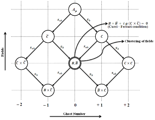
Figure 1: (Anti-)BRST symmetry transformations for the non-Abelian 1-form gauge field, associated (anti-)ghost fields and emergence of CF condition.

captures these transformations geometrically. We note that, in the whole diagram, there is a single point, at the ghost number zero, where there is a clustering of the auxiliary fields $B\equiv B\cdot T$ and $\bar{B}\equiv\bar{B}\cdot T$, which emerge from the (anti-)BRST symmetry transformations on the ghost fields $C\equiv C\cdot T$ and anti-ghost fields $\bar{C}\equiv\bar{C}\cdot T$, respectively. This is the place where the CF condition exists as it connects these auxiliary Nakanishi-Lautrup fields, $B$ and $\bar{B}$, with the ghost number zero object constructed from the fermionic (anti-)ghost fields $(\bar{C})C$ of the theory (i.e., $B+\bar{B}+i\;g\;(C\times\bar{C})=0$).

In our earlier works on the 4D Abelian 2-form and 6D 3-form gauge theories, [18, 19] we have explained the existence and emergence of the (anti-)BRST invariant CF-type restrictions by exploiting the fundamental notions of geometry and group theory from pure mathematics. As a warm-up exercise in ref. 19, we have also considered the existence of CF condition for the 4D non-Abelian 1-form gauge theory within the framework of BRST formalism by taking the help of concepts from pure mathematics. In our present endeavor, we claim that, for any arbitrary $p$-form gauge theory within the framework of BRST formalism, it is the symmetry transformations that would provide us the clue for the existence of CF-type conditions in the theory. In fact, wherever, in the above type of diagram (Fig. A1), there is clustering of different variety of fields at a particular ghost number, there will emerge a CF-type condition (which will be mathematically connected with the idea of gerbes [18, 19]). Thus, physically, we interpret the mathematical object gerbes as some artifact that connects the fields, which cluster at a particular ghost number (in the diagram like Fig. A1 for a given theory) and they basically prove the linear independence (i.e. the absolute anticommutativity) of the BRST and anti-BRST symmetries.

The hallmark of a gauge theory, at the classical level, is the existence of first-class constraints on them in the language of Dirac’s prescription for classification scheme. On the other hand, one of the decisive features of a gauge theory, at the quantum level, is the existence of CF-type conditions (which are mathematically backed by the idea of gerbes) within the realm of BRST approach.

References

• [1] D. Z. Freedman and P. K. Townsend. Nucl. Phys. B, 177, 282 (1981).
• [2] T. J. Allen, M. J. Bowick and A. Lahiri. Mod. Phys. Lett. A, 6, 559 (1991).
• [3] A. Lahiri. Phys. Rev. D, 63, 105002 (2001).
• [4] E. Harikumar, A. Lahiri and M. Sivakumar. Phys. Rev. D, 63, 105020 (2001).
• [5] S. Gupta and R. P. Malik. Eur. Phys. J. C, 58 , 517 (2008).
• [6] S. Gupta, R. Kumar and R. P. Malik Eur. Phys. J. C, 65, 311 (2010).
• [7] S. Gupta, R. Kumar and R. P. Malik. Eur. Phys. J. C, 70, 491 (2010).
• [8] R. Kumar and R. P. Malik. Eur. Phys. Lett. 94, 11001 (2011).
• [9] R. Kumar and R. P. Malik. Eur. Phys. J. C, 71, 1710 (2011).
• [10] S. Krishna, A. Shukla and R. P. Malik. Int. J. Mod. Phys. A, 26, 4419 (2011).
• [11] R. Jackiw and S-Y. Pi. Phys. Lett. B, 403, 297 (1997).
• [12] S. Deser, R. Jackiw and S. Templeton. Phys. Rev. Lett. 48, 975 (1982).
• [13] S. Deser, R. Jackiw and S. Templeton. Ann. Phys. (NY), 140, 372 (1982).
• [14] J Schwinger. Phys. Rev. 125, 397 (1962).
• [15] J. Schwinger. Phys. Rev. 128, 2425 (1962).
• [16] Ö. F. Dayi. Mod. Phys. Lett. A, 13, 1969 (1998).
• [17] O. M. Del Cima. J. Phys. A: Math. Theor. 44, 352001 (2011).
• [18] L. Bonora and R. P. Malik. Phys. Lett. B, 655, 75 (2007).
• [19] L. Bonora and R. P. Malik. J. Phys. A: Math. Theor. 43, 375403 (2010).
• [20] I. Ojima. Prog. Theo. Phys. 64, 625 (1980).
• [21] S. Hwang. Nucl. Phys. B, 322, 107 (1989).
• [22] S. Hwang. Nucl. Phys. B, 231, 386 (1984).
• [23] L. Bonora and M. Tonin. Phys. Lett. B, 98, 48 (1981)
• [24] L. Bonora, P. Pasti and M. Tonin. Nuovo Cimento A, 63, 353 (1981).
• [25] R. P. Malik. J. Phys. A: Math. Theor. 40, 4877 (2007).
• [26] R. P. Malik. Eur. Phys. J. C, 51, 169 (2007).
• [27] R. P. Malik. Eur. Phys. J. C, 47, 277 (2006).
• [28] G. Curci and R. Ferrari. Phys. Lett. B, 63, 91 (1976).
• [29] I. A. Batalin, P. M. Lavrov and I. V. Tyutin. J. Math. Phys. 31, 6 (1990).
• [30] I. A. Batalin, P. M. Lavrov and I. V. Tyutin. J. Math. Phys. 31, 1487 (1990).
• [31] P. M. Lavrov. Phys. Lett. B, 366, 160 (1996).
• [32] E. Witten. Mod. Phys. Lett. A, 5, 487 (1990).
• [33] S. Gupta and R. Kumar. Mod. Phys. Lett. A, 28, 1350011 (2013).
• [34] S. Weinberg. The Quantum Theory of Fields: Modern Applications. Vol. 2. Cambridge University Press, Cambridge. 1996.
• [35] R. P. Malik and T. Pradhan. Z. Phys. C, 28, 525 (1985).
• [36] O. M. Del Cima, Phys. Lett. B, 720, 254 (2013).
• [37] S. Gupta and R. Kumar. Manuscript in preparation.