Phase transitions in optical turbulence

Abstract

We consider turbulence in the Gross-Pitaevsky model and study the creation of a coherent condensate via an inverse cascade originated at small scales. The growth of the condensate leads to a spontaneous breakdown of symmetries of small-scale over-condensate fluctuations: first, statistical isotropy is broken, then series of phase transitions mark the change of symmetry from the two-fold to three-fold to four-fold. At the highest condensate level reached, we observe a short-range positional and long-range orientational order (similar to a hexatic phase in the condensed matter physics). In other words, the longer one pumps the system the more ordered it becomes. We show that these phase transitions happen when the driving term corresponds to an instability (i.e. it is multiplicative in the ${\bf k}$-space) but not when the system is pumped by a random force. Thus we demonstrate for the first time non-universality of the inverse-cascade turbulence. We also describe anisotropic spectral flux flows in ${\bf k}$-space, anomalous correlations of fluctuations and collective oscillations of turbulence-condensate system.

I Introduction

Probably the most unexpected discovery made in the study of turbulence is an inverse cascade. Flying at the face of an intuitive picture of turbulence as the process of fragmentation and dissipation, inverse cascade means self-organization, i.e. appearance of large-scale motions out of a small-scale noise. The process of inverse cascade culminates in the creation of spectral condensate i.e. a mode coherent across the whole system. At this point turbulence shares many properties with quantum physics as displaying both fluctuations and coherence. This closeness shows perhaps most vividly in the studies on non-equilibrium states within the framework of Nonlinear Schrödinger (or Gross-Pitaevsky) Equation, called here NSE. In the realm of classical physics, this model describes spectrally narrow distribution of nonlinear waves, the respective far-from-equilibrium states are called optical turbulence ZLF ; Naz ; Fal . For quantum physics, this is the simplest model of locally interacting bosons. The Hamiltonian and the canonical NSE are as follows

$${\cal H}=\int\Bigl{(}|\nabla\psi|^{2}+|\psi|^{4}/2\Bigr{)}\,d^{2}r\,,$$ (1)

$$i\psi_{t}=\nabla^{2}{\cal H}/\delta\psi^{*}=-\Delta\psi+|\psi|^{2}\psi\ .$$ (2)

To provide for a turbulent inverse cascade, we add medium-scale pumping and small-scale dissipation and solve the resulting equation numerically with a record spatial and temporal resolution. We address the central issue in the non-equilibrium physics, i.e. that of universality: to what extent the properties of a far-from-equilibrium state depend on the excitation mechanism? Theoreticians prefer to pump a turbulent system by a random Gaussian force, which practically never can be met in real systems where waves usually appear as a result of some instability. Here we consider both ways to excite waves (additive random forcing and instability) and show that they produce similar turbulence only when the condensate is weak. We show that the instability-excited system undergoes a series of phase transitions to the states with different symmetries while the force-driven system does not.

Understanding the interaction of turbulence and a coherent flow is an important problem in turbulence studies in fluid mechanics and beyond, both from fundamental and practical perspectives. In fluids, coherent flows are system-size vortices or zonal flows of different profiles Shats ; CKL , which are known to diminish the turbulence level, change its nature and make its statistics more non-Gaussian Shats ; NP . Here we consider arguably the simplest case of a turbulent system with a condensate: the coherent part is expected to be a constant field and turbulence to consist of weakly interacting waves. We carry our simulations well past time when all vortices, i.e. holes in the condensate, disappear (due to annihilations no ) and observe that the coherent part contains a small but important spatial structure and the turbulence is not effectively weak. As a result, this simple system demonstrates unexpectedly rich behavior with novel features never before observed in turbulence systems.

II Theoretical considerations

Let us denote $N=\overline{|\psi|^{2}}$ and $N_{0}=|\overline{\psi}|^{2}$. In what follows the overline means average over space, and the averages over time we shall denote by angular brackets. The total number of waves with nonzero wave numbers is $N-N_{0}=n=\int|\psi_{k}|^{2}d^{2}k$.

The simplest condensate is a spatially-uniform field, $A=\sqrt{N_{0}}\exp(-iN_{0}t)$, which is an exact solution of (2). Small over-condensate fluctuations satisfy

$$i\dot{\psi}_{k}=(k^{2}+2N_{0})\psi_{k}+A^{2}\psi_{-k}^{*}.$$ (3)

This equation gives the Bogolyubov dispersion relation,

$$\Omega_{k}^{2}=2N_{0}k^{2}+k^{4}\ ,$$ (4)

for a pair of counter-propagating waves $\psi_{k}\propto\exp(-iN_{0}t-i\Omega_{k}t)$, $\psi_{-k}^{*}\propto\exp(iN_{0}t-i\Omega_{k}t)$.

II.1 Turbulence with the condensate

As the condensate grows, the dispersion relation (4) approaches the acoustic one with the sound velocity $c=\sqrt{2N_{0}}$. As known, acoustic waves running at the same direction interact strongly (producing shocks). On the other hand, the effective matrix element of the three-phonon interaction behaves as $|V_{123}|^{2}\simeq k_{1}k_{2}k_{3}/N_{0}^{1/2}$ (see e.g. Opt ). One can estimate the mean value of the cubic term in the Hamiltonian using the weak-turbulence approximation ZLF :

$$\langle{\cal H}_{3}\rangle\! = \sum_{{\bf k}_{1},{\bf k}_{2},{\bf k}_{3}}V_{123}\langle\psi_{k_{1}}\psi_{k_{2}}\psi_{k_{3}}^{*}\rangle\delta(\mathbf{k}_{1}+\mathbf{k}_{2}-\mathbf{k}_{3})$$ (5)

$$\simeq \!\!\!\!\!\!\sum_{{\bf k}_{1},{\bf k}_{2},{\bf k}_{3}}\!\!\!\!\!|V_{123}|^{2}n_{1}n_{2}\,\delta({\bf k}_{1}+{\bf k}_{2}-{\bf k}_{3})\delta(\Omega_{1}+\Omega_{2}-\Omega_{3})$$

$$\simeq {|V|^{2}n^{2}c\over k^{3}}{k\over c}\simeq{n^{2}k\over N_{0}^{1/2}}\ .$$

Here we have introduced the mean spectral density of waves also called the normal correlation function $n_{k}=\langle|\psi_{k}|^{2}\rangle$. The factor ${k/c}$ in (5) is the effective angle of interaction that can be estimated considering $\Omega_{k}\approx c|k|+k^{3}/2c\approx ck+ck_{\perp}^{2}/2k+k^{3}/2c$ and comparing diffraction and dispersion corrections: $k_{\perp}/k\simeq k/c$. We then estimate $\langle{\cal H}_{2}\rangle\simeq ckn$ and obtain the effective nonlinearity parameter for over-condensate phonons as the ratio:

$${{\cal H}_{3}\over{\cal H}_{2}}\simeq{n\over N_{0}}\ .$$ (6)

This suggests that when the number of waves with zero momentum outgrows the number of waves with nonzero momentum, nonlinear interaction must be getting effectively weak despite the fact that the nonlinear term in the Hamiltonian is dominant. The estimate (6) explains the observation made in DF that the statistics of the fluctuations is non-Gaussian at low condensate values but is getting closer to Gaussian, as the condensate grows.

Formula (5) allows also to estimate the typical rate of a local nonlinear interaction (i.e. for waves with comparable $k$) as $1/t_{nl}(k)\simeq|V|^{2}n_{k}k^{2}(c/k^{3})(k/c)\simeq n_{k}k/N_{0}^{1/2}$. The rate of nonlinear interaction $1/t_{nl}$ decreases as the condensate grows. Therefore, nonlocal interactions must play more and more important role. Here we define the coherent part as the field filtered at the frequency $N$ and show that it is not a constant but has a rather elaborate spatial structure. Interaction of turbulence and the coherent part (nonlocal in ${\bf k}$-space) is responsible for the set of new phenomena described below.

One may think that an effective weak nonlinearity expressed by (6) allows one to describe the over-condensate turbulence by the weak turbulence theory i.e. by a closed kinetic equation written for the one-time (normal) correlation function $n_{k}$. We will see here that this is not necessarily the case. The crucial point is that validity of weak turbulence approach requires not only weak nonlinearity but random phases as well. We show below (analytically) that condensate imposes phase coherence, the most straightforward manifestation of which is the existence of anomalous correlation functions and the phase coherence of the $k,-k$-pairs with the condensate. We then describe the series of phase transitions (discovered by the direct numerical simulations) that show evolution towards more and more ordered state as the condensate grows; such evolution cannot be described by a kinetic equation, which satisfies H-theorem and can describe only entropy growth.

II.2 Anomalous correlations

Let us now show that an important element of turbulence against the background of a condensate must be anomalous correlations, i.e. phase coherence between waves running in opposite directions (seems to have been overlooked so far). Indeed, the existence of the condensate must produce the anomalous correlation function $\langle\psi_{k}\psi_{-k}\rangle\propto\exp(-2iN_{0}t)$. To look into the effective dynamics of both the number of waves and the condensate, let us assume for simplicity that only two contra-propagating waves with amplitudes $\psi_{\pm k}=\sqrt{n_{\pm k}}\exp(-iN_{0}t+i\,\phi_{\pm k})$ interact with the condensate and expand the Hamiltonian (1) up to the terms quadratic in $\psi_{\pm k}$. That gives the equations:

$$\begin{split}{dn_{k}\over dt}&=-\frac{1}{2}\,{dN_{0}\over dt}=-B=2N_{0}\sqrt{n_{k}n_{-k}}\sin(2\phi_{0}-\phi_{k}-\phi_{-k})\,,\\ {dB\over dt}&=4(2n_{k}+2n_{-k}-N_{0}-k^{2})C+8N_{0}n_{k}n_{-k}\\ &-2N_{0}^{2}(n_{k}+n_{-k})\,,\\ {dC\over dt}&=(N_{0}+k^{2}-2n_{k}-2n_{-k})B\end{split}$$

where we have denoted $A^{2}\psi_{k}^{*}\psi_{-k}^{*}=C-iB/2$. We see that the steady state corresponds to $B=0$ and $C=-N_{0}\sqrt{n_{k}n_{-k}}$ that is to $2\phi_{0}-\phi_{k}-\phi_{-k}=\pi$ (and $n_{k}=n_{-k}=k^{2}/2$). Alternatively, one calculates the time derivative of the Hamiltonian, quadratic in $A,\psi_{\pm k}$: $d{\cal H}_{2}/dt\approx 4N_{0}Im(A^{2}4\psi_{-k}^{*}\psi_{k}^{*})=N_{0}^{2}\sqrt{n_{k}n_{-k}}\sin(2\phi_{0}-\phi_{k}-\phi_{-k})$, which is the energy flux from the condensate to the wave pair with $k,-k$. The flux turns to zero and the steady state is established when the phase of the pair is exactly opposite to the phase of $A^{2}$, which plays the role of an effective pumping.

II.3 Anisotropy of turbulence

At the beginning, waves in the pumping shell are pumped isotropically. Eventually, the inverse cascade reaches lowest modes, which have the four-fold symmetry of the box. Let us now discuss what possible anisotropy may turbulence spectra acquire after the condensate appears. Just looking at the Bogolyubov dispersion relation (4) one may suggest the following scenario: spatial modulation of the condensate intensity $N_{0}$ means respective modulation of the sound velocity for shorter waves. Standing waves corresponding to the lowest modes of the box provide such modulation. Regions of low sound velocity would act as waveguides with short waves moving predominantly along the minima of $N_{0}$. That suggests that for sufficiently high $N_{0}$, when (4) is close to linear, the angular maxima at high $k$ would correspond to minima at low $k$ for a hypothetical anisotropic spectrum. In other words, acoustic waves interact effectively when they are collinear, so the maximum of long waves at some angle effectively removes short waves from the pumping region at that angle. That consideration suggests a simple picture of possible anisotropy: lowest modes have the symmetry of the square box and impose that symmetry on the small-scale turbulence (turned by $\pi/4$). The main result of this work is that this is not the case.

III Numerical procedure

Our numerical simulations are set up similarly to DF . We use 4th order fully dealiased split-step method agrawal ; yoshida to solve Eq. (2) in the presence of forcing,

$$i\,\psi_{t}=-\nabla^{2}\,\psi+|\psi|^{2}\,\psi+i\hat{\gamma}\,\psi.$$ (7)

The forcing consists of large scale pumping and small scale damping. The pumping-attenuation operator $\hat{\gamma}$ is local in the ${\bf k}$-space and is given by $\gamma(k)=\gamma_{p}(k)-\gamma_{d}(k)$ where the pumping is non-zero only within the shell DF ,

$$\gamma_{p}(k)=\alpha\,\sqrt{(k^{2}-k_{l}^{2})(k_{r}^{2}-k^{2})}\quad\mathrm{at}\quad k_{l}<k<k_{r}$$

and the damping is of Landau-type,

$$\gamma_{d}(k)=\beta\,k^{2}\,h(k/k_{d}),$$

where function $h(x)$ is defined as

$$h(x)=\left\{\begin{array}[]{cc}(6\,x^{5})^{-1}\,\exp\left[5\,(1-x^{-2})\right],&x\leq 1;\\ &\\ 1-(5/6)\,\exp\left[(1/2)\,(1-x^{2})\right],&x>1.\end{array}\right.$$

The pumping shell $[k_{l},k_{r}]$ is relatively narrow and occupies the middle of the computational domain. Note that we do not suppress long wave excitations (no damping is present at $k=0$) so, as expected, the condensate starts to form early on and the total number of waves begins to grow in time. As in DF , the initial condition is given by thermal equilibrium spectrum, $n_{k}=T/(k^{2}+\mu)$, with random phases.

The values for simulation parameters are shown in Table 1. Note that the size of the box, $L$, increases with resolution, while forcing remains the same. As a result the number of waves per unit area, $N$, evolves in a similar way in simulations at different box sizes, see Figure 1a. Unless specified, the results are shown below for the run A.

box size $L$	$2\pi$	$4\pi$	$8\pi$
resolution	$128$	$256$	$512$
timestep	$10^{-4}$	$10^{-4}$	$10^{-4}$
$\sqrt{\mu}$	0.15	0.3	0.6
initial $NL^{2}$	15	60	240
forcing: $k_{l}$	28	56	112
forcing: $k_{r}$	32	64	128
forcing: $k_{d}$	42	84	168
forcing: $\beta$	$10\alpha$	$10\alpha$	$10\alpha$
forcing: $\alpha$
run A	$6.40\times 10^{-2}$	$1.60\times 10^{-2}$	$4.00\times 10^{-3}$
run B	$3.20\times 10^{-2}$	$8.00\times 10^{-3}$	$2.00\times 10^{-3}$
run C	$1.60\times 10^{-2}$	$4.00\times 10^{-3}$	$1.00\times 10^{-3}$
run D	$8.00\times 10^{-3}$	$2.00\times 10^{-3}$	$5.00\times 10^{-4}$

Table 1: Note: (a) resolution is shown excluding dealiased modes; (b) the timestep is reduced to $5\times 10^{-5}$ when $\max|\psi|^{2}$ reaches $2\times 10^{3}$, and to $2\times 10^{-5}$ when $\max|\psi|^{2}$ reaches $4\times 10^{3}$.

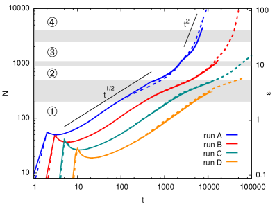
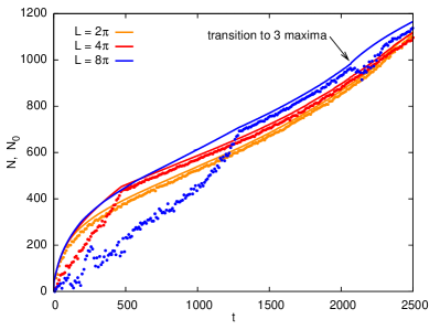
Figure 1: Left: Number of waves as a function of time in $L=2\pi$ (dashed lines) and $L=4\pi$ (solid lines) simulations, also rescaled as $\epsilon$. Gray regions correspond to the transition between regimes; circled labels refer to the number of jets (petals). Right: Appearance of condensate in simulations with different box sizes in Run A. The condensate value $N_{0}$ is shown by dots, next to the lines representing $N$. The initial linear growth of the condensate at strong forcing and large boxes is accompanied by creation and destruction of vortices. When vortices die out, $N_{0}$ catches up with $N$.

To collect better statistics, we occasionally stop the simulation and restart it with uniform friction which stabilizes the condensate growth and leads to a steady state. In this case, the forcing is replaced by $\tilde{\gamma}=\gamma-b$, where $b$ is constant determined empirically to stabilize $N$ at a given level.

To study the structure of the coherent mode and fluctuations separately, we applied the time-spectral filtering used by Nazarenko and Onorato no . After the condensate appears, the frequency spectrum has a sharp peak at $\omega_{0}=N$. We select a time window containing many $2\pi/\omega_{0}$ periods (typically 100) and store the temporal evolution of the $\psi(r,t)$ with 12-24 time-slices per period. This data is transformed to $\omega$-$k$ space, where the coherent mode — slice corresponding to $\omega_{0}$ — is separated. The rest of the frequency spectrum we treat as fluctuations.

We use as a measure of nonlinearity, the dimensionless parameter $\epsilon=N\lambda^{2}/4$ where $\lambda$ is the pumping wavelength, which is not only the smallest scale in the inverse cascade but also the smallest scale in the system since dissipation dominates for the scales less than $\lambda$. All our simulations are done with the same $\lambda\approx 2\pi/30$, so $\epsilon$ also has the meaning of rescaled number of waves, $\epsilon\approx 0.01N$.

IV Results and discussion

IV.1 Condensate growth

The nonlinear interaction conserves the total number of waves so the latter grows only due to net pumping: $dN(t)/dt=\Gamma(t)=\int\gamma_{k}n_{k}(t)\,d^{2}k$. A simple expectation would be that $N(t)$ must initially grow exponentially as a result of linear instability, then nonlinearity saturates this growth. After $n_{k}$ stabilizes in the pumping region, one expects a linear law $N=\Gamma t$. The first study of the wave number growth was done in DF where it was observed that nonlinearity indeed slows it down (and for a while even reverses) after the initial exponential increase. The following assertions were then made in  DF : (a) the first nonlinear stage of growth follows the law $N\propto\sqrt{t}$, which means that the occupation numbers in the pumping shell decrease as $n_{k}\propto 1/\sqrt{t}$; (b) the square-root regime starts when the number of waves at the condensate is of order of the total number of waves; (c) the square-root regime ends when $\epsilon\simeq 1$ i.e. the correlation scale $N_{0}^{-1/2}$ is approaching the pumping scale; (d) after that, $n_{k}$ stabilizes and $N=\Gamma t$ with time-independent $\Gamma$. As seen from the Figure 1 (left panel) (produced at the resolutions much higher and on time intervals much longer than those of DF ), the evolution, which we observe, does not follow this simple scenario. At earlier times, the growth on average can be crudely approximated as $\sqrt{t}$. In some simulations, we observed a transitional linear regime, as in DF . It can be seen on a linear scale, as, for instance, the section $500<t<1800$ for $L=8\pi$ curve in Figure 1 (right panel). At later times, the growth rate of the condensate accelerates even faster than linear, with possible transition to the ultimate regime $N\propto t^{2}$ regime hypothesized by Zakharov and Nazarenko ZN . The growth $N(t)$ is determined by the number of waves in the pumping shell, and we shall see in the next section that this number evolves in a complicated way due to phase transitions. We found the law of this growth sensitive to different parameters and were not able to distinguish any definite scaling. That subject definitely requires extensive future studies.

IV.2 Phase transitions

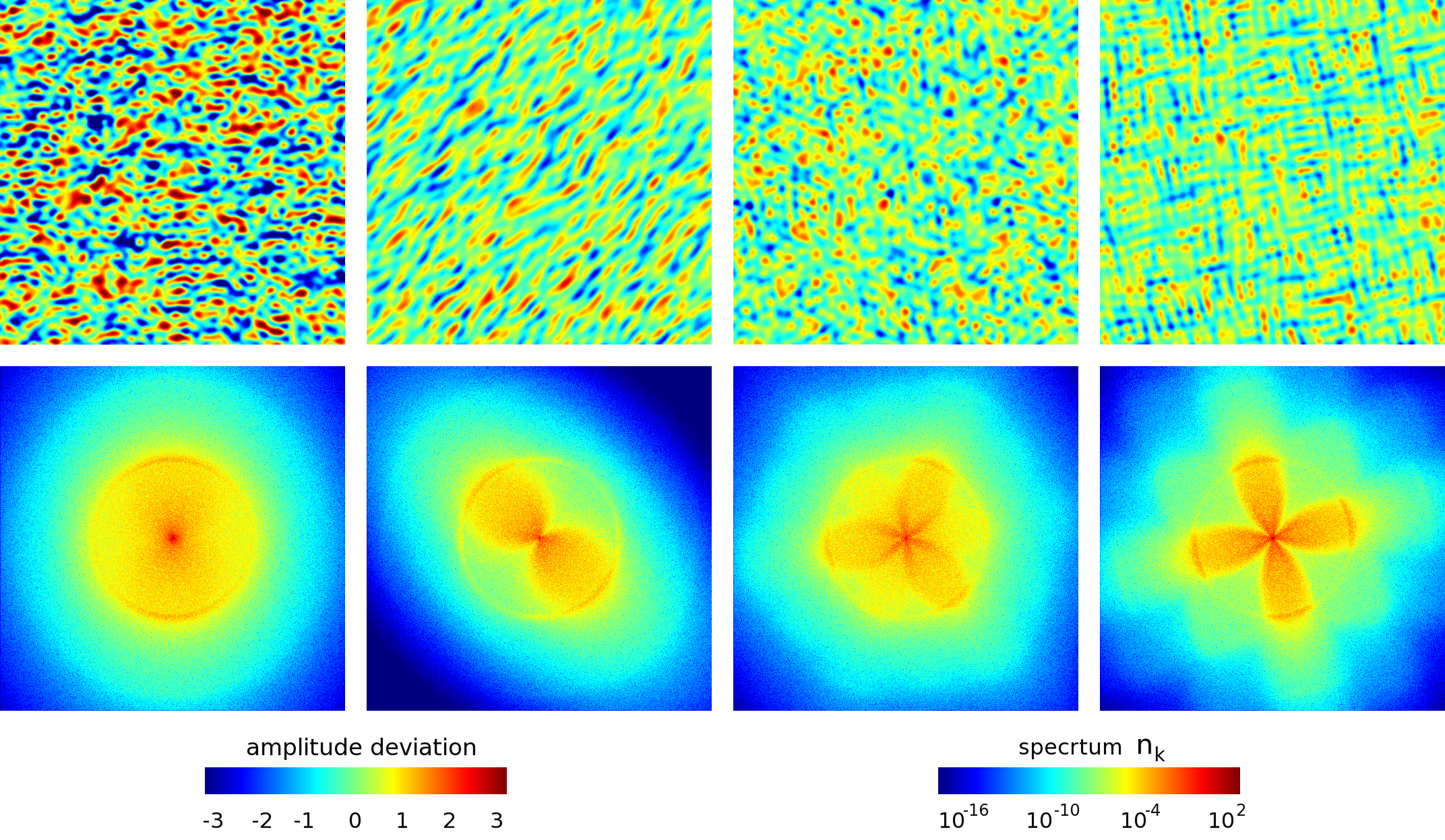
Figure 2: Amplitude deviation from average in a $2\pi\times 2\pi$ part of the computational domain (above) and $n_{k}$ spectrum (below) in $L=8\pi$ simulation. From left to right images correspond to $t=100$, $1500$, $2500$, and $7500$ ($N=219$, 771, 1166, 4202, $\epsilon=2.40$, 8.45, 12.77, 46.08).

transition		two-fold to three-fold			three-fold to four-fold
run	$L$	$t$	$N$	$\epsilon$	$t$	$N$	$\epsilon$
A	$2\pi$	$2150\pm 50$	$932\pm 23$	$10.22\pm 0.25$	$6250\pm 50$	$3910\pm 70$	$42.88\pm 0.77$
	$4\pi$	$2350\pm 50$	$1053\pm 24$	$11.55\pm 0.27$	$7350\pm 50$	$4310\pm 65$	$47.30\pm 0.71$
	$8\pi$	$2050\pm 50$	$979\pm 26$	$10.74\pm 0.29$	$7150\pm 50$	$3830\pm 57$	$42.00\pm 0.63$
B	$2\pi$	$13500\pm 500$	$1025\pm 45$	$11.23\pm 0.50$	$31500\pm 500$	$2578\pm 79$	$28.28\pm 0.87$
	$4\pi$	$15250\pm 50$	$1010\pm 5$	$11.08\pm 0.05$	N/A
C	$2\pi$	$99500\pm 500$	$1378\pm 7$	$15.12\pm 0.07$	N/A

Table 2: Time, the number of waves, and nonlinearity parameters at phase transitions.

Initially, condensate is fed by an inverse cascade carried by an almost isotropic spectrum of fluctuations. At this stage, the nonlinear (interaction) term in the Hamiltonian is less or comparable to the quadratic term (which describes dispersion for waves or kinetic energy for particles). As condensate grows, the first symmetry breaking appears at $\epsilon\simeq 1$ and the system becomes anisotropic — the amplitude and the phase develop patterns on the scale of the forcing and larger; the spectrum turns into an oval. The transformation happens gradually, in the interval $2\lesssim\epsilon\lesssim 5$, as the oval slowly becomes thinner at the waist.

As the condensate amplitude grows further, we observe the sequence of phase transitions: at first the oval spectrum turns into a dumbbell, then the symmetry changes from two-fold (two-petal) to three-fold and then to four-fold, as seen in Figure 2. Further transitions are possible. While we could not evolve our runs to higher levels of condensate, we observed other symmetries in the simulations with different initial conditions (discussed below). In Figure 1 (left panel) we have shown the regions of transitions as gray bands in the plot of $\epsilon(t)$. The transitions are accompanied by an increase in the variance of the over-condensate excitations, $n=N-N_{0}$, as seen from the Figure 1(right panel).

The transition times and condensate amplitudes are listed in Table 2 for different pumping powers and box sizes. The transitions occur sharply yet the threshold values of $\epsilon$ fluctuate from realization to realization, as we find in the simulations which only differ in the phases of initial thermal noise (see Figure 3.) This shows that we are not dealing with a linear instability with a well-defined threshold. Indeed, the condensate is stable with respect to the infinitesimal perturbations. It is likely that our transitions are of probabilistic nature similar to transitions in a pipe flow Hof or fiber laser tur when with the change of a control parameter (condensate amplitude in our case) one changes the probability that a finite-amplitude perturbation will lead the system away to a new state.

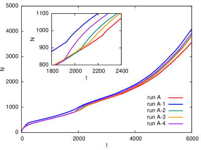
Figure 3: The transition from 2 to 3 petals, seen as the kink in $N(t)$, for different random phases of the initial condition. The insert plot is the zoom to the kink area. One can see 10% difference in $N$ at the moment of transition.

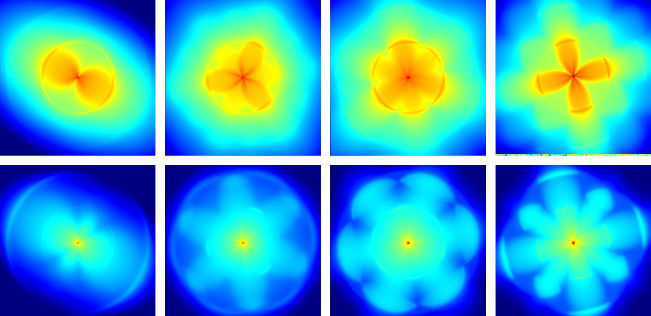
Figure 4: Total spectrum (above) and filtered spectrum of the coherent mode (below) in $L=8\pi$ simulation. From left to right images correspond to $t=1500$, $2100$, $6500$ and $7500$ ($N=771$, 1005, 3102, 4202). The averaging was done over 100 time units in stabilized runs. Colormap is the same as in Figure 2.

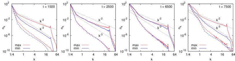
Figure 5: Radial dependency at two directions (first row) and angular dependency at $|k|=8$, 24, 48, 64 (second row, from top to bottom) for the spectra shown in Figure 4. Dashed lines in the radial spectra correspond to the coherent mode.

It can be recognized in the second, third, and fourth panels of the second row in Figure 5 that the maxima at high $k$ correspond to minima at low $k$, in agreement with the waveguide argument presented in Section II.3. However, the symmetry of the spectra both at low and high $k$ is definitely not that of a box. The minima and maxima are directed at different angles and the spectrum of turbulence can have three-fold symmetry that is not that of a square box. Bottom row of Figure 4 shows that the mode coherently oscillating with the frequency $N$ has an intricate spatial structure and multiscale correlations the anisotropy of which is directly related to the anisotropy of over-condensate fluctuations. The spectrum of the coherent mode has the doubled number of maxima and is generally more symmetric than the whole spectrum, as seen from Figure 4. For nonzero momenta, over-condensate fluctuations dominate over the coherent part.

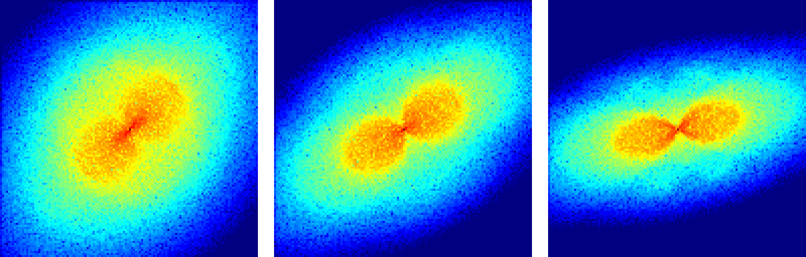
Figure 6: Form of the spectrum at $t=10000,40000,80000$, from left to right, in Run C at $L=2\pi$. The spectrum angular width decreases as $N$ grows.

In addition to phase transitions between different symmetry states, the spectra undergo slow evolution between transitions. The intensity fluctuates, the whole structure may slowly rotate or swing. With time, two-petal spectra concentrate in a more narrow angle, as seen in Figure 6, and broaden again just before the transition. The three-petal spectra broaden with time, especially at high $k$. The third columns in Figures 4,5 show spectra just before the transition, when they become close to six-petal; the seeds of the new (four-fold) symmetry visible at low $k$ in the coherent part, as seen in Figure 7. The population of the pumping shell increases between the transitions and falls during the transitions, which explains a complicated character of the evolution of the total number of waves.

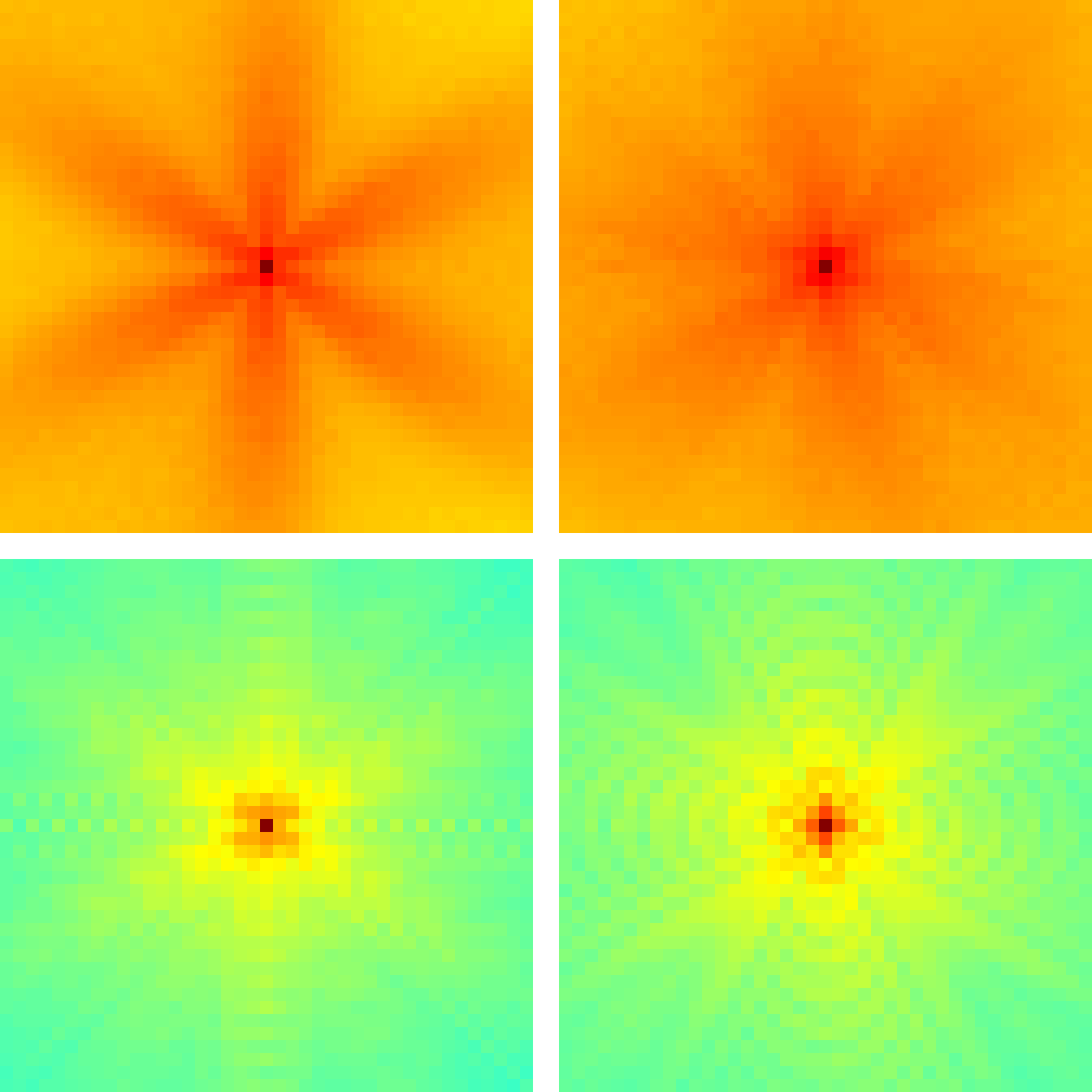
Figure 7: Zoom into the central part of the total spectra (above) and the spectra for the coherent mode (below) for $L=4\pi$ and $t=3000,6000$; both correspond to three-fold symmetry. One can see the four-fold symmetry appearing at low $k$ in the lower right panel.

At any moment, except possibly very close to the transition events, and for all symmetries, the angular width of the spectra decreases towards larger wavenumbers, as seen in Figures 4, 5. This may be analogous to spectrum anisotropization observed for acoustic turbulence ZLF ; FM . It is worth stressing the difference in two cases: acoustic turbulence studied there corresponds to a direct energy cascade (realized by pumping-generated long waves turning into shocks), while here we have an inverse cascade. One can therefore say that as an inverse cascade proceeds towards larger wavelength, the spectra are getting wider as weak turbulence theory would predict ZLF ; yet presently we see no way it can predict the spontaneous appearance of anisotropy and changes in symmetry, particularly, significant anisotropy at the pumping scale.

One may suggest a possible physical mechanism of phase transitions as follows: phonons effectively interact only within the angle $k/\sqrt{N_{0}}$, which decreases as $N_{0}$ grows, so the turbulence tends to be broken into jets. The number of jets $j$ increases proportionally to the inverse of the interaction angle i.e. as $N_{0}^{1/2}\propto\epsilon^{1/2}$. Indeed, we observe that the transitions happen approximately at $\epsilon_{j}\sim j^{2}$. Even if this is indeed the basic mechanism of the transitions, we still lack any understanding of whether there is a unifying principle that can predict which turbulent state is realized the way variational principle does it for thermal equilibrium. One direction worth exploring is whether one can develop an approach similar to the weak crystallization theory KLM despite the fact the we are dealing with developed turbulence and power-law spectra carrying flux in ${\bf k}$-space, as seen in Figs 5, 11 below.

Finally, we made separate runs taking initial conditions for $\psi$ as a thermal noise plus large constant (pre-existing condensate). In these cases, the same states (with 2,3,4 petals) appear i.e. they are true attractors, independent of the history. We also observed 6-petal spectra with triangular spatial pattern in the amplitude, and 8-petal spectra with the spatial distribution comprised of patches of square patterns oriented at 45 degree angle. The 6-petal spectra was observed at higher $\epsilon$ than 4-petal spectra, although pre-existing condensate makes all thresholds lower and possibly less sensitive to the phases of the initial thermal noise. We speculate that this is because in the runs with a pre-existing condensate, the spectrum first develops a uniformly populated pumping shell which is then free to break apart into the appropriate number of jets, contrary to evolving systems where the previous configuration has to re-populate the pumping shell. The ability of the system to quickly find its equilibrium state opens horizons for a much more extensive exploration of parameter space, which hopefully will be a subject of future studies.

IV.3 Orientational order

For two-fold and three-fold spectra, turbulence statistics is translational invariant. The most remarkable finding is seen at the last image of the top row in Figure 2: on top of a long-range orientational order, a short-range positional order appears. This state is between the solid and the isotropic liquid very much like hexatic phase in 2d melting Hex . It requires future detailed studies to establish whether this is indeed a turbulent analog of the Berezinski-Kosterlitz-Thouless transition; to avoid misunderstanding, let us stress that there are no vortices (holes) in the condensate at this stage, the phase fluctuates weakly; it is the small condensate perturbations which are getting ordered. These spatial correlations are also seen in Figure 8 which shows the correlation function of the amplitude, $\overline{\psi({\bm{x}})\psi({\bm{x}}+{\bm{r}})}-\overline{\psi}^{2}$, where overline means averaging over the position ${\bm{x}}$.

The type of crystallization that we observe is very much different from the vortex crystallization with a wavelength externally imposed by a cut-off in 2d incompressible turbulence SY .

Figure 8: Correlation function of the amplitude of the over-condensate fluctuations at $t=7500$ for $L=2\pi$.

IV.4 Anomalous correlations and collective oscillations

As we have predicted above (Section II.2) anomalous correlations must exist between any two contra-propagating waves. In our direct numerical simulations we have confirmed that this is true at least for the two lowest modes of the box, their total phase is indeed shifted by $\pi$ relative to the condensate. These modes give the main contribution of the collective oscillations of the system which are periodic conversions of waves from condensate to over-condensate with the total number of waves unchanged.

We checked that in the numerical data the steady-state anomalous correlation function indeed has the phase shifted by $\pi$ relative to the condensate value squared. For example, for $L=4\pi$ and $N=570$, the modes that have the largest amplitudes, with $(k_{x},k_{y})=(1,0),(1,1),(1,-1)$, have their phase differences $(\phi_{k}+\phi_{-k}-2\phi_{0})/\pi=1.01,1.02,0.99$ respectively.

It was noticed in Fal84 that when broad turbulent spectra coexist with a sharp spectral peak these two groups of waves generally have different relaxation times which makes possible oscillations about a steady state. For three-wave interaction, an integral model (of a predator-prey type) that describes the evolution of the total numbers of waves in the two groups has the form: $dN_{0}/dt=-bN_{0}+N_{0}n$, $dn/dt=\gamma n-N_{0}n$, which gives the oscillations with the frequency $\sqrt{\gamma b}=\sqrt{\bar{n}\bar{N_{0}}}$ Fal84 .

The oscillations for NSE with a condensate were reported in Opt where a similar model was suggested: $dN_{0}/dt=-bN_{0}+N_{0}n^{2}$, $dn/dt=\gamma n-N_{0}^{2}n$. This model gives the steady-state values $\bar{N_{0}}=\sqrt{\gamma}$, $\bar{n}=\sqrt{b}$ and the same frequency of oscillations $\sqrt{\gamma b}=\sqrt{\bar{n}\bar{N_{0}}}$. The most evident defect of the latter model is that it does not conserve the total number of waves, moreover, the steady-state values are wrong too (in reality, $\bar{N}_{0}\propto 1/b$ while $\bar{n}$ is practically independent of $b$ in wide intervals). We notice here that to describe the collective oscillations of the turbulence-condensate system, one needs to account properly for the anomalous correlation function, as was done while deriving system (II.2). In particular, our suggested system does describe the oscillations around a steady state. Consider, $N_{0}=\bar{N}_{0}+M$, $n_{k}=\bar{n}_{k}+m$, assuming that the steady-state values satisfy $\bar{N}_{0}\gg\bar{n}_{k}$. We then get

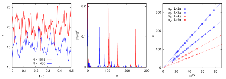
Figure 9: Left: oscillations in over-condensate in Run A, $L=2\pi$ box, zoomed around times $t^{\prime}=800$ ($N=486$) and $t^{\prime}=3500$ ($N=1518$). Middle: frequency spectrum of the time-dependence of the number of over-condensate waves for the same run in time intervals $[800,810]$ and $[3500,3510]$. Right: first two frequencies as function of the number of waves in $L=2\pi$ and $L=4\pi$ boxes. Dashed lines have the slopes 4, $2\sqrt{2}$, 2, $\sqrt{2}$.

$$\begin{split}{dm\over dt}&=-b=-{dM\over 2dt}\,,\\ {dB\over dt}&=-4(\bar{N}_{0}+k^{2})C-4\bar{N}_{0}^{2}m\,,\\ {dC\over dt}&=(\bar{N}_{0}+k^{2})B\end{split}$$

Figure 10: Oscillations of number of waves in the condensate, $N_{0}$, and in the coherent mode for $L=2\pi$.

The system above describes collective oscillations with twice the Bogolyubov frequency: $M,m,B,C\propto\exp(-i\,\Omega t)$, $\Omega=2\Omega_{k}=2\sqrt{2\bar{N}_{0}k^{2}+k^{4}}$. Indeed, numerical simulations show that the oscillations have frequencies that are equal to twice that of the lowest modes of the Bogolyubov spectrum. For the box with $L=2\pi$ we find that the modulus of the anomalous correlation functions $\sigma(k_{x},k_{y})=\sigma(1,0)$ and $\sigma(1,1)$ oscillate respectively with the frequencies $2\sqrt{2N_{0}}$ and $4\sqrt{N_{0}}$. These frequencies (which are much smaller than the frequency of the condensate $N$) essentially do not depend on the level of over-condensate fluctuations, they are clearly seen in the oscillations of the condensate amplitude and of the normal correlation functions shown in Figure 9. As seen from Figure 10, the total number of waves is unchanged. The number of over condensate waves (about $40=6080-6040$) consists of a coherent part (about $10=6050-6040$), the rest (about 30) are waves with other frequencies. Note that the number of over-condensate waves exceeds substantially the amplitude of the oscillations (about 5). The oscillations can be thus treated in a linearized approximation.

IV.5 Moments, spectra and flux lines

Table 3 shows the integral statistical characteristics of over-condensate fluctuations for different times and levels of the condensate. We define $\delta\psi=\psi-\bar{\psi}$ and compute the spatial averages of its moments. The fourth column gives the second moment, which is the fraction of waves with nonzero wavenumbers: $\overline{|\delta\psi|^{2}}/N_{0}=(N-N_{0})/N_{0}$. The last column shows the flatness, which is close to the Gaussian value 3. Far from the transitions, the flatness is actually somewhat lower than 3 and decreases as the condensate grows, i.e. the condensate effectively suppresses strong over-condensate fluctuations contrary to what condensate vortices do to 2D incompressible turbulence Shats . Only for $t=6500$, which is close to the three-to-four transition, we find flatness slightly exceeding 3, i.e. somewhat stronger fluctuations. Note in passing that the coherent mode at all scales has substantially smaller flatness, which means that strong fluctuations of the mode are even more rare than for a Gaussian random quantity.

$t\quad$	$N\quad$	$N_{0}\quad$	$\;\overline{|\delta\psi|^{2}}/N_{0}\;$	$\;\overline{\,|\delta\psi|^{4}}/\left(\overline{\,|\delta\psi|^{2}}\right)^{2}$
1500	771	751	0.027	2.95
2500	1166	1133	0.029	2.67
6500	3102	2871	0.080	3.17
7500	4200	3986	0.054	2.40

Table 3: Integral statistics of fluctuations corresponding to spectra in Figures 4,5.

Let us stress that despite anomalous correlations, symmetry-breaking phase transitions and collective oscillations (all properties normally associated with narrow spectra in ${\bf k}$-space), our spectra are wide along and across the jets, decaying approximately by power laws, as seen in Figure 5. Note that $1/k^{2}$ is the spectrum of weak turbulence inverse cascade which coincides in this case (up to a logarithmic factor) with the thermal equilibrium, while $1/k^{3}$ is the spectrum due to the shock waves.

Let us now describe the lines of the flux that these spectra carry towards the condensate. Conservation of waves allows one to write NSE as a continuity equation and define the flux, ${\bf J}_{k}$, via the relation ${\rm div}{\bf J}_{k}=\langle|\psi_{k}|^{2}\rangle\,\gamma_{k}\equiv Q_{k}$. In this Poisson equation, $Q_{k}$ plays the role of a charge density and the flux plays the role of potential. We compute $Q_{k}$ and solve the above equation. Figure 11 shows the flux lines while positive/negative source $Q_{k}$ is shown by red/blue regions.

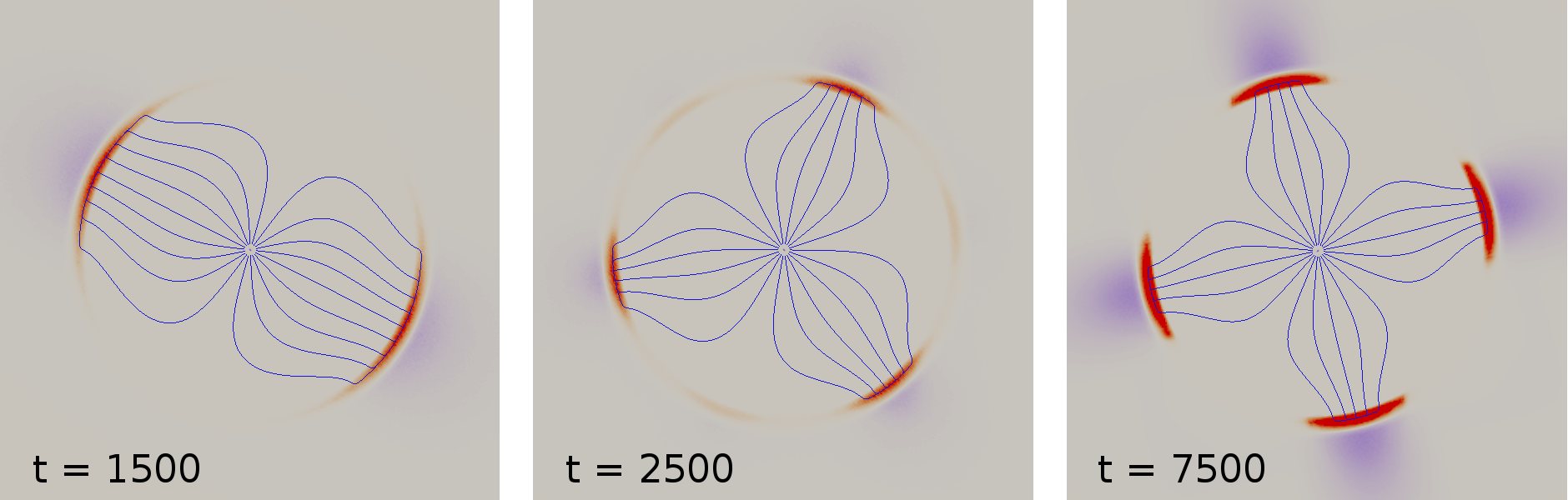
Figure 11: Source distribution and flux flow lines at $t=1500$, $t=2500$, and $t=7500$ for $L=8\pi$.

IV.6 Non-universality of the inverse cascade turbulence

It is important that the phase transitions happen only when the waves are excited by an instability. If we excite waves by an additive random force concentrated in the same ring in ${\bf k}$-space with about the same amplitude, turbulence remains close to isotropic at all wavenumbers exceeding unity and at all condensate levels, as seen in Fig 12. To the best of our knowledge, this is the first demonstration of significant non-universality of turbulence with respect to excitation mechanism. It is particularly striking that we find it for an inverse cascade which is generally particularly robust sym . Apparently, the condensate-turbulence interaction can make turbulence non-universal.

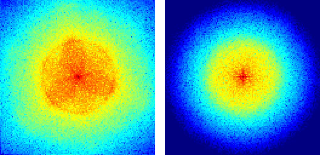
Figure 12: Spectra for an instability (left) and the random force (right) at about the same levels of condensate for $L=2\pi$. One sees that force-driven turbulence remains isotropic except for a few box-size modes, while the instability-driven turbulence develops a three-petal spectrum in the whole of ${\bf k}$-space.

This set of simulations was performed for $L=2\pi$ and the following procedure was used. First a run with an instability excitation was done with the initial condition as a large constant (corresponding to $N_{0}=1000$) plus small thermal noise. The run was stopped after it produced a 3-petal spectrum shown in the left panel of Fig. 12; during that time the total number of waves grew only by 3.6% from its initial value. Second, a run with an additive forcing was performed. In this run the multiplicative term $\gamma_{p}(k)\psi_{k}$ was replaced by an additive forcing $f({\bf k},t)$ (the multiplicative damping term, $\gamma_{d}(k)$, was preserved). This forcing term was non-zero only inside the pumping shell $k_{l}\leq k\leq k_{r}$, it had random phases uniformly distributed in the interval $[0,2\pi]$ and uncorrelated both in ${\bf k}$-space and time. Its amplitude was chosen to be constant $|f({\bf k},t))|=f$ the value of which was determined by a condition that both additive and multiplicative forcing have the same average amplitude in the $\bf{k}$-space:

$$f=\frac{1}{\pi(k_{r}^{2}-k_{l}^{2})}\,\int_{k_{l}\leq k\leq k_{r}}\,\gamma_{p}(k)\,|\psi_{k}|\,d^{2}k\ .$$

To conclude, discerning guiding principles that govern the physics far from equilibrium remain elusive. Is there any quantity (similar to entropy) that the system tries to optimize by undergoing the series of phase transitions described here?

We thank A. Zamolodchikov, V. Lebedev, E. Kats, A. Finkelstein and B. Shraiman for helpful discussions. This research was supported by the grants of the BSF, ISF and by the Minerva Foundation funded by the German Ministry for education and research. Part of the work was done at KITP where it was supported by the National Science Foundation under Grant NSF PHYS-51164. Computations were done at the New Mexico Computing Application Center and at UNM Center for Advanced Research Computing.

References

- (1) V. E. Zakharov, V.S. L’vov and G. Falkovich, Kolmogorov Spectra of Turbulence (Springer 1992).
- (2) S. Nazarenko, Wave Turbulence (Springer 2011).
- (3) G. Falkovich, Fluid Mechanics, a short course for physicists (Cambridge Univ. Press 2011)
- (4) H. Xia, M. Shats and G. Falkovich, Phys. Fluids 21, 125101 (2009).
- (5) M. Chertkov et al, Phys. Rev. Lett. 99, 084501 (2007).
- (6) H. Xia et al, Nature Physics 7, 321 (2011).
- (7) S.Nazarenko, M.Onorato, Physica D 219, 1 (2006); J. Low. Temp. Phys. 146, 31 (2007).
- (8) S. Dyachenko et al, Physica D 57, 96 (1992).
- (9) A. Dyachenko and G. Falkovich, Phys. Rev. E 54, 5095 (1996).
- (10) G. P. Agrawal, Nonlinear Fiber Optics ( Academic Press, San Diego, 2007).
- (11) H. Yoshida, Phys. Lett. A 150, 262 (1990).
- (12) V. E. Zakharov and S.V. Nazarenko, Physica D 201, 203 (2005).
- (13) K. Avila et al, Science 333, 192 (2011).
- (14) E. Turitsyna et al, Phys. Rev. A 80, 031804(R) (2009).
- (15) G. Falkovich and M. Meyer, Phys. Rev E 54, 4431 (1995).
- (16) E. I. Kats, V. V. Lebedev and A.R Muratov, Phys. Rep. 228, 1 (1993).
- (17) J.M. Kosterlitz and D.J. Thouless, J. Phys. C 5, L124 (1972); J. Phys. C 6, 1181 (1973).
- (18) L. Smith and V. Yakhot, J Fluid Mech. 214, 115 (1994).
- (19) G. Fal’kovich, Radiophys. Quant. Elec. 27, 122 (1984).
- (20) G. Falkovich, J Phys A 42, 123001 (2009).