Mixture latent autoregressive models for longitudinal data

Abstract

Many relevant statistical and econometric models for the analysis of longitudinal data include a latent process to account for the unobserved heterogeneity between subjects in a dynamic fashion. Such a process may be continuous (typically an AR(1)) or discrete (typically a Markov chain). In this paper, we propose a model for longitudinal data which is based on a mixture of AR(1) processes with different means and correlation coefficients, but with equal variances. This model belongs to the class of models based on a continuous latent process, and then it has a natural interpretation in many contexts of application, but it is more flexible than other models in this class, reaching a goodness-of-fit similar to that of a discrete latent process model, with a reduced number of parameters. We show how to perform maximum likelihood estimation of the proposed model by the joint use of an Expectation-Maximisation algorithm and a Newton-Raphson algorithm, implemented by means of recursions developed in the hidden Markov literature. We also introduce a simple method to obtain standard errors for the parameter estimates and a criterion to choose the number of mixture components. The proposed approach is illustrated by an application to a longitudinal dataset, coming from the Health and Retirement Study, about self-evaluation of the health status by a sample of subjects. In this application, the response variable is ordinal and time-constant and time-varying individual covariates are available.

Keywords: Expectation-Maximisation algorithm; Hidden Markov model; Latent Markov model; Proportional odds model; Quadrature methods.

1 Introduction

In the analysis of longitudinal data, an important aspect that can be accounted for is the unobservable heterogeneity between subjects. This form of heterogeneity corresponds to the effect that unobservable factors have on the occasion-specific response variables in addition to the effect of observable covariates. The simplest approach to account for the unobserved heterogeneity is based on the inclusion, in the model of interest, of individual-specific random intercepts, that can have either a continuous or a discrete distribution. Models based on individual parameters having a continuous distribution may be casted in the class of Generalised Linear Mixed models and that of Random Effects models (see Snijders and Bosker,, 1999; McCulloch and Searle,, 2001; Goldstein,, 2003; Skrondal and Rabe-Hesketh,, 2004; Hancock and Samuelson,, 2008). Models based on discrete random effects may be seen as forms of Latent Class (LC) models (Lazarsfeld,, 1950; Lazarsfeld and Henry,, 1968; Goodman,, 1974; Bandeen-Roche et al.,, 1997; Huang and Bandeen-Roche,, 2004). See also Hagenaars and McCutcheon, (2002) for an exhaustive review about the LC model.

The approaches mentioned above assume that the effect of unobservable factors on the response variables is time constant. A more general assumption consists of introducing, for each subject, time-varying individual random effects which give rise to a latent process for the unobserved heterogeneity. Even in this case we can disentangle the continuous case from the discrete case. The most common formulation based on a continuous-valued latent process assumes that the individual effects follow an Autoregressive model of order 1 (AR(1)); see Chi and Reinsel, (1989) and Heiss, (2008). Hereafter, this model is referred to as Latent Autoregressive (LAR) model. On the other hand, models based on a discrete latent process typically assume that the individual effects follow a first-order Markov chain. A Latent Markov (LM) model (Wiggins,, 1973) with covariates results; see Bartolucci et al., (2010) for a review.

The debate on which is more appropriate, between the continuous and the discrete latent process formulation, is open. The first formulation is usually more easy to justify from a theoretical point of view; in principle, there is no reason to consider the effect of unobserved factors as discrete. Moreover, a LAR model has a parsimony close to that of the corresponding continuous random effect model (with time-constant individual effects), since it represents the latent structure by only two parameters: correlation index and variance of the individual effects. However, the model estimation may be computationally problematic (Heiss,, 2008). On the other hand, discrete latent variable models may reach a better fit to the analysed data. In particular, the LM model may be seen as a semi-parametric model because, with the suitable number of states, the underlying Markov chain may approximate any (even continuous) process with a first order dependence structure. This advantage is at the cost of a reduced parsimony, since the number of parameters increases with the square of the number of states. Moreover, the interpretation may be more difficult for the same reason mentioned above: it is more natural to consider the effect of unobservable factors or covariates as continuous than discrete.

A debate similar to that described above, between a continuous and a discrete formulation for the latent process, is also present in the literature on models for item responses (Hambleton and Swaminathan,, 1985); see, for among others, Lindsay et al., (1991). A similar debate is also present in the literature about the analysis of certain types of time-series data. In particular, for the analysis of financial data, the Stochastic Volatility (SV) model (Taylor,, 1982; Shephard,, 1996) may be used as an alternative to the hidden Markov (HM, MacDonald and Zucchini,, 1997) model. For an interesting comparison between the two approaches see Taylor, (1999) and for a comprehensive review see Taylor, (2005). The SV model represents the volatility by an AR(1) process, and then has a structure that recalls that of the LAR model for longitudinal data, whereas the HM model relies on a Markov chain, and then it is very similar to the LM model. In the field of time-series data, which is strongly related to that of longitudinal data, we also have to mention Markov-switching models (see Frühwirth-Schnatter,, 2006, Ch. 9-10). In this field, the interest is also on the the possibility to combine a continuous with a discrete approach; see, among others, Kitagawa, (1987), Cai, (1994), Hamilton and Susmel, (1994), So et al., (1998), and Rossi and Gallo, (2006). Although the similarities between the typical formulations of models for time series and longitudinal data, to our knowledge no attempts to combine continuous and discrete process formulations have been made in the context of longitudinal data.

In this paper, we propose a model for longitudinal data which is based on a mixture of latent AR(1) processes to account for the unobserved heterogeneity between subjects in a dynamic fashion. Each component of the mixture has its own mean and correlation coefficient, but these components have a common variance. The proposed model, which can be used with response variables of a different nature (binary, ordinal, or continuous), belongs to the class of continuous latent process models for longitudinal data. As such, it retains the natural interpretation that characterises the LAR model, but it reaches a better fit to the data, since it generalises this model. In particular, the goodness of fit to the data may reach levels close that those of the LM model, but with a reduced number of parameters.

In order to make inference on the proposed model, we show how to compute its likelihood function by a recursion taken for the hidden Markov literature (Baum et al.,, 1970; MacDonald and Zucchini,, 1997); a procedure results which is equivalent to the Sequential Gaussian Quadrature (SGQ) method proposed by Heiss, (2008). Through recursions similar to those used for HM models, we also implement an Expectation-Maximisation (EM) algorithm and a Newton-Raphson (NR) algorithm for the maximisation of the likelihood function and, therefore, for the estimation of the model parameters. The NR algorithm is based on the observed information matrix which is obtained by the same numerical method proposed by Bartolucci and Farcomeni, (2009). This matrix is also exploited to obtain standard errors for the parameter estimates. Finally, we show how to obtain the prediction of the individual effect for every subject in the sample at each time occasion. Through these predictions we define a criterion to choose the number of components to be used in data analysis. We recall that each component corresponds to a separate AR(1) latent process.

The advantages of the proposed approach are illustrated through an application to a longitudinal dataset concerning the self-evaluation of health status at eight different time periods. The dataset is derived from the the Health and Retirement Study conducted by the University of Michigan. In this case, the response variable observed at each occasion has five ordered categories. The proposed model is implemented by specifying a proportional odds model for global logits. Some observed covariates related with individual characteristics are also included. The model selected for these data is compared with the corresponding LAR and LM models.

The paper is organised as follows. In the next section we introduce the basic notation and describe some relevant approaches for longitudinal data. In Section 3 we outline the proposed model for longitudinal data and, in Section 4, we describe likelihood based inference for this model. The results of the application based on the self evaluation of health status data are illustrated in Section 5. Final conclusions are reported in the Section 6.

2 Preliminaries

With reference to a sample of $n$ subjects observed at $T$ time occasions, let $y_{it}$ be the response variable for subject $i$ at occasion $t$ and let $\mbox{\boldmath$x$}_{it}$ be a corresponding column vector of covariates, with $i=1,\ldots,n$ and $t=1,\ldots,T$. We also denote by $\mbox{\boldmath$y$}_{i}=(y_{i1},\ldots,y_{iT})$ the vector of response variables and by $\mbox{\boldmath$X$}_{i}=\begin{pmatrix}\mbox{\boldmath$x$}_{i1}&\cdots&\mbox{\boldmath$x$}_{iT}\end{pmatrix}$ the matrix of all covariates for subject $i$.

At this stage, we do not restrict the response variable to have a specific nature. Therefore, we introduce a latent continuous variable $y_{it}^{*}$ underlying each $y_{it}$. In particular, we assume that

$$y_{it}=G(y_{it}^{*}),$$ (1)

where $G(\cdot)$ is a parametric function which may depend on specific parameters according to the different nature of $y_{it}$, such as specific cutpoints in the presence of ordinal variables. Hereafter, we use $\mbox{\boldmath$y$}_{i}^{*}=(y_{i1}^{*},\ldots,y_{iT}^{*})$ to denote the vector of latent response variables corresponding to $\mbox{\boldmath$y$}_{i}$. More details about the possible formulations of $G(\cdot)$ will be given in Section 3.1.1.

In the following, we briefly review models which allow us to take into account the unobserved heterogeneity between subjects by introducing time-constant and time-varying individual effects.

2.1 Models with time-constant individual effects

The simplest approach to take into account the unobserved heterogeneity is based on the assumption that, for every unit $i$, the latent response variables in $\mbox{\boldmath$y$}_{i}^{*}$ are conditionally independent given the covariates $\mbox{\boldmath$X$}_{i}$ and an individual-specific intercept $\alpha_{i}$ (local independence). Moreover, it is assumed that each $y_{it}^{*}$ only depends on $\alpha_{i}$ and $\mbox{\boldmath$x$}_{it}$ as follows

$$y_{it}^{*}=\alpha_{i}+\mbox{\boldmath$x$}_{it}^{\prime}\mbox{\boldmath$\beta$}+\varepsilon_{it},\quad i=1,\ldots,n,\>t=1,\ldots,T,$$ (2)

where the error terms $\varepsilon_{it}$ are assumed mutually independent and identically distributed. Note that each vector $\mbox{\boldmath$x$}_{it}$ may also include the lagged response.

When the individual-specific intercepts $\alpha_{i}$ are treated as random parameters, the same distribution (usually independent of the covariates) is assumed for all subjects, which may be continuous or discrete. In the first case, we typically assume that $\alpha_{i}\sim N(0,\sigma^{2})$ for $i=1,\ldots,n$. In the second case, instead, every $\alpha_{i}$ may assume a value among $k$ possible values or support points $\xi_{h}$ having probabilities $\pi_{h}$, with $h=1,\ldots,k$. The support points and the corresponding probabilities are typically estimated on the basis of the data, which also drive the choice of $k$. A first model of this type is known as finite mixture of regression models, which is an extension of a mixture of normal distributions with averages expressed as functions of the explanatory variables (Quandt,, 1972; Quandt and Ramsey,, 1978).

In any case, the assumption of conditional independence of the response variables given the individual-specific intercepts and the covariates allows us to write

$$p(\mbox{\boldmath$y$}_{i}|\alpha_{i},\mbox{\boldmath$X$}_{i})=\prod_{t}p(y_{it}|\alpha_{i},\mbox{\boldmath$x$}_{it}),\quad i=1,\ldots,n,$$ (3)

where $p(y_{it}|\alpha_{i},\mbox{\boldmath$x$}_{it})$ denotes the probability mass or density function of $y_{it}$, given $\alpha_{i}$ and $\mbox{\boldmath$x$}_{it}$, which, in turn, depends on the adopted parameterisation; see equations (1) and (2). Then, under the random effect approach, the manifest distribution of $\mbox{\boldmath$y$}_{i}$ given $\mbox{\boldmath$X$}_{i}$ is obtained by marginalising the probability or density in (3) with respect to $\alpha_{i}$. With continuous random effects, we have

$$p(\mbox{\boldmath$y$}_{i}|\mbox{\boldmath$X$}_{i})=\int p(\mbox{\boldmath$y$}_{i}|\alpha_{i},\mbox{\boldmath$X$}_{i})f(\alpha_{i})d\alpha_{i}=\int\bigg{[}\prod_{t}p(y_{it}|\alpha_{i},\mbox{\boldmath$x$}_{it})\bigg{]}f(\alpha_{i})d\alpha_{i},$$

where $f(\alpha_{i})$ is the probability density function of every $\alpha_{i}$, which may depend on a specific parameter vector. With discrete random effects, instead, we have

$$p(\mbox{\boldmath$y$}_{i}|\mbox{\boldmath$X$}_{i})=\sum_{h}\bigg{[}\prod_{t}p(y_{it}|\xi_{h},\mbox{\boldmath$x$}_{it})\bigg{]}\pi_{h}.$$

This distribution is the base for constructing a marginal likelihood to be maximised in order to estimate the model parameters.

2.2 Models based on time-varying individual effects

The main drawback of the individual-specific random intercept models described above is that they assume the effect of unobservable factors to be time constant. This assumption may be relaxed by the inclusion of individual-time-specific effects $\alpha_{it}$, $i=1,\ldots,n$, $t=1,\ldots,T$. In an obvious way, the assumption of local independence is extended by assuming that, for all sample units $i$, the latent response variables in $\mbox{\boldmath$y$}_{i}^{*}$ are conditionally independent given $\mbox{\boldmath$\alpha$}_{i}=(\alpha_{i1},\ldots,\alpha_{iT})$ and $\mbox{\boldmath$X$}_{i}$. Moreover, assumption (2) is naturally extended as follows

$$y_{it}^{*}=\alpha_{it}+\mbox{\boldmath$x$}_{it}^{\prime}\mbox{\boldmath$\beta$}+\varepsilon_{it},\quad i=1,\ldots,n,\>t=1,\ldots,T.$$ (4)

Given the model complexity, time-varying effects may only be assumed to be random and not fixed. Again, two alternative approaches, continuous and discrete, are available in the literature. The most common continuous random-effects approach assumes that every $\mbox{\boldmath$\alpha$}_{i}$ follows an AR(1) process, so that

$$\alpha_{i1} = \varepsilon_{i1},$$

$$\alpha_{it} = \alpha_{i,t-1}\rho+\varepsilon_{it}\sqrt{1-\rho^{2}},\quad t=2,\ldots,T,$$

where $\varepsilon_{it}\sim N(0,\sigma^{2})$, $t=1,\ldots,T$. This is the LAR formulation already mentioned in Section 1, which was studied in detail by Heiss, (2008).

The discrete latent process formulation assumes that, for all $i$, $\mbox{\boldmath$\alpha$}_{i}$ follows a first-order homogenous Markov chain with $k$ states denoted by $\xi_{1},\ldots,\xi_{k}$. This chain has initial probabilities $\pi_{h}$ and transition probabilities $\pi_{h_{1}h_{2}}$, with

$$\pi_{h} = p(\alpha_{i1}=\xi_{h}),\quad h=1,\ldots,k,$$ (5)

$$\pi_{h_{1}h_{2}} = p(\alpha_{i,t-1}=\xi_{h_{1}},\alpha_{it}=\xi_{h_{2}}),\quad h_{1},h_{2}=1,\ldots,k,\>t=2,\ldots,T.$$ (6)

In other words, it is assumed that every $\alpha_{it}$ is conditionally independent of $\alpha_{i1},\ldots,\alpha_{i,t-2}$ given $\alpha_{i,t-1}$, but apart from this assumption, the distribution of $\mbox{\boldmath$\alpha$}_{i}$ is unconstrained. On the other hand, this greater flexibility corresponds to a higher number of parameters to estimate with already $k\geq 2$. In fact, the number of parameters involved in the Markov chain (support points and initial and transition probabilities) is equal to $(k-1)+(k-1)+k(k-1)=k^{2}+k-2$, taking into account the constraints $\sum_{h}\pi_{h}=1$ and $\sum_{h_{2}}\pi_{h_{1}h_{2}}=1$, $h_{1}=1,\ldots,k$, and that to ensure identifiability one constraint has to be put on the support points. This is a formulation of LM type, which was exploited by Bartolucci and Farcomeni, (2009) to propose a flexible class of models for multivariate categorical longitudinal data. We have to mention that, in order to make easier the comparison between the LAR and the LM model, we can require that the initial probabilities $\pi_{h}$ in (5) coincide with those of the stationary distribution of the chain. In this case, we have a moderate reduction of the number of parameters which becomes equal to $k^{2}-1$.

Under both the continuous and the discrete latent process formulations, the assumption of local independence implies that

$$p(\mbox{\boldmath$y$}_{i}|\mbox{\boldmath$\alpha$}_{i},\mbox{\boldmath$X$}_{i})=\prod_{t}p(y_{it}|\alpha_{it},\mbox{\boldmath$x$}_{it}).$$

Moreover, under the first formulation, which leads to the LAR model, the manifest distribution of $\mbox{\boldmath$y$}_{i}$ given $\mbox{\boldmath$X$}_{i}$ has probability mass (or density) function

$$p(\mbox{\boldmath$y$}_{i}|\mbox{\boldmath$X$}_{i})=\int p(\mbox{\boldmath$y$}_{i}|\mbox{\boldmath$\alpha$}_{i},\mbox{\boldmath$X$}_{i})f(\mbox{\boldmath$\alpha$}_{i})d\mbox{\boldmath$\alpha$}_{i}.$$ (7)

This is an integral over the $T$-dimensional space of $\mbox{\boldmath$\alpha$}_{i}$ that may be difficult to compute in practice. At this aim, we can use the SGQ method proposed by Heiss (2008), which is essentially based on rewriting expression (7) as follows

$$p(\mbox{\boldmath$y$}_{i}|\mbox{\boldmath$X$}_{i}) = \int p(y_{i1}|\alpha_{i1},\mbox{\boldmath$x$}_{i1})f(\alpha_{i1})\int p(y_{i2}|\alpha_{i2},\mbox{\boldmath$x$}_{i2})f(\alpha_{i2}|\alpha_{i1})\cdots$$ (8)

$$\cdots\int p(y_{iT}|\alpha_{iT},\mbox{\boldmath$x$}_{iT})f(\alpha_{iT}|\alpha_{i,T-1})d\alpha_{iT}\cdots d\alpha_{i2}d\alpha_{i1}$$

and then sequentially computing the integral involving each single random effect $\alpha_{it}$, where $f(\alpha_{i1})$ refers to the distribution of $\alpha_{i1}$ and $f(\alpha_{it}|\alpha_{i,t-1})$ to the distribution of $\alpha_{it}$ given $\alpha_{i,t-1}$, $t=2,\ldots,T$.

When a latent Markov chain is assumed, the manifest distribution of $\mbox{\boldmath$y$}_{i}$ given $\mbox{\boldmath$X$}_{i}$ is defined as follows

$$p(\mbox{\boldmath$y$}_{i}|\mbox{\boldmath$X$}_{i})=\sum_{h_{1}}p(y_{i1}|\xi_{h_{1}},\mbox{\boldmath$x$}_{i1})\pi_{h_{1}}\sum_{h_{2}}p(y_{i2}|\xi_{h_{2}},\mbox{\boldmath$x$}_{i2})\pi_{h_{1}h_{2}}\cdots\sum_{h_{T}}p(y_{iT}|\xi_{h_{T}},\mbox{\boldmath$x$}_{iT})\pi_{h_{T-1}h_{T}}.$$ (9)

In order to efficiently compute this sum, we can exploit a forward recursion (Baum et al.,, 1970; Dempster et al.,, 1977) which is well known in the hidden Markov literature (MacDonald and Zucchini,, 1997). See Bartolucci, (2006) and Bartolucci et al., (2010) for an efficient implementation in matrix notation.

3 Proposed model

In this section, we describe the proposed model for longitudinal data, which is based on a mixture of AR(1) processes to account for the unobserved heterogeneity in a dynamic fashion. We name this model as Mixture Latent Autoregressive model, indicated for short by MLAR or by MLAR($k$) when we want to mean a specific number of mixture components $k$.

3.1 Model assumptions

The proposed model is based on the following assumptions for $i=1,\ldots,n$:

• the latent response variables in $\mbox{\boldmath$y$}_{i}^{*}$, and therefore the observed response variables in $\mbox{\boldmath$y$}_{i}$, are conditionally independent given $\mbox{\boldmath$X$}_{i}$ and a latent process $\mbox{\boldmath$\alpha$}_{i}=(\alpha_{i1},\ldots,\alpha_{iT})$;

• every response variable $y_{it}^{*}$ in $\mbox{\boldmath$y$}_{i}^{*}$, and then every $y_{it}$ in $\mbox{\boldmath$y$}_{i}$, only depends on $\alpha_{it}$ and $\mbox{\boldmath$x$}_{it}$ through a parameterisation formulated on the basis of (1) and (4);

• the latent process $\mbox{\boldmath$\alpha$}_{i}$ has distribution given by a mixture of $k$ AR(1) processes with common variance $\sigma^{2}$.

Assumptions A1 is the usual assumption of local independence already discussed in Section 2.2; the other two assumptions are discussed in detail below.

3.1.1 Assumption A2

The introduction of an underlying continuous outcome $y_{it}^{*}$ related to the observed response variable $y_{it}$ as specified in (1), allows us to adapt the model to several situations. Indeed, depending on the assumed distribution for the errors $\varepsilon_{it}$ in (4) and on the specification of $G(\cdot)$ different models result.

The simplest case is when we let $G(y^{*})=y^{*}$, that is the identity function, and $\varepsilon_{it}\sim N(0,\sigma^{2})$ for all $i$ and $t$. In this case, a model results in which

$$y_{it}|\alpha_{it},\mbox{\boldmath$x$}_{it}\sim N(\alpha_{it}+\mbox{\boldmath$x$}_{it}^{\prime}\mbox{\boldmath$\beta$},\sigma^{2}),\quad i=1,\ldots,n,\>t=1,\ldots,T.$$

This is the typical formulation adopted with continuous response variables.

When the response variables are binary, that is $y_{it}=0,1$, we typically assume that $G(y^{*})=I\{y^{*}>0\}$, where $I\{\cdot\}$ is an indicator function assuming value 1 when its argument is true and value 0 otherwise. Depending on the distribution of the error term $\varepsilon_{it}$ in model (4), a logit or probit parameterisation results. More precisely, if we assume a logistic distribution for the error terms $\varepsilon_{it}$, then a logit parameterisation results, under which

$$\log\frac{p(y_{it}=1|\alpha_{it},\mbox{\boldmath$x$}_{it})}{p(y_{it}=0|\alpha_{it},\mbox{\boldmath$x$}_{it})}=\alpha_{it}+\mbox{\boldmath$x$}_{it}^{\prime}\mbox{\boldmath$\beta$},\quad i=1,\ldots,n,\>t=1,\ldots,T.$$ (10)

The probit version of this model is obtained by assuming that $\varepsilon_{it}\sim N(0,1)$, so that:

$$\Phi^{-1}\{p(y_{it}=1|\alpha_{it},\mbox{\boldmath$x$}_{it})\}=\alpha_{it}+\mbox{\boldmath$x$}_{it}^{\prime}\mbox{\boldmath$\beta$},\quad i=1,\ldots,n,\>t=1,\ldots,T,$$

with $\Phi(\cdot)^{-1}$ denoting the inverse of the standard Normal cumulative distribution function.

Finally, an interesting case (that we consider in the application illustrated in Section 5) is when each response variable $y_{it}$ is ordinal with categories $1,\ldots,J$. In this case we can introduce a set of cutpoints $\mu_{1}\leq\cdots\leq\mu_{J-1}$ and formulate the function in (1) as

$$G(y^{*})=\left\{\begin{array}[]{cc}1&y^{*}\leq\mu_{1},\\ 2&\mu_{1}<y^{*}\leq\mu_{2},\\ \vdots&\vdots\\ J&y^{*}>\mu_{J-1}.\end{array}\right.$$

In analogy with the binary case, an ordered logit or an ordered probit parameterisation results according to whether the error terms $\varepsilon_{it}$ have a logistic or a standard Normal distribution, respectively. In the first case, we have that

$$\log\frac{p(y_{it}\geq j|\alpha_{it},\mbox{\boldmath$x$}_{it})}{p(y_{it}<j|\alpha_{it},\mbox{\boldmath$x$}_{it})}=\mu_{j}+\alpha_{it}+\mbox{\boldmath$x$}_{it}^{\prime}\mbox{\boldmath$\beta$},\quad i=1,\ldots,n,\>t=1,\ldots,T,\>j=2,\ldots,J.$$ (11)

This parameterisation is based on global or cumulative logits, the same logits used in the Odds Proportional model of McCullagh, (1980). Note that, as in this model, we are assuming that the effect of the covariates ($\mbox{\boldmath$x$}_{it}^{\prime}\mbox{\boldmath$\beta$}$) and of the unobserved individual parameters ($\alpha_{it}$) do not depend on the specific response category ($j$); this assumption could be removed, but the model would become more complex to estimate and to interpret. Finally, note that parameterisation (11) is a generalisation of that in (10) for binary variables.

3.1.2 Assumption A3

In order to formulate this assumption, we introduce, for $i=1,\ldots,n$, the discrete latent variable $u_{i}$ which has $k$ support points, indexed from 1 to $k$, and mass probabilities $\pi_{1},\ldots,\pi_{k}$. Then, we assume that

$$\alpha_{i1}=\xi_{u_{i}}+\varepsilon_{i1},\quad i=1,\ldots,n,$$

and that

$$\alpha_{it}=\xi_{u_{i}}+(\alpha_{i,t-1}-\xi_{u_{i}})\rho_{u_{i}}+\varepsilon_{it}\sqrt{1-\rho_{u_{i}}^{2}},\quad i=1,\ldots,n,\>t=2,\ldots,T,$$

where $\varepsilon_{it}\sim N(0,\sigma^{2})$ for all $i$ and $t$. In the above expressions, $(\xi_{h},\rho_{h})$ is a pair of parameters related to the latent state $u_{i}$ that, for $h=1,\ldots,k$, have to be estimated jointly with the common variance $\sigma^{2}$. In order to ensure the identifiability of the model, we require that $\xi_{1}=0$ or, alternatively, $\sum_{h}\xi_{h}\pi_{h}=0$. The number of parameters for the latent structure becomes equal to $(k-1)+k+(k-1)=3k-2$, which can be directly compared with those defined for the LAR and LM models in Section 2.2.

An equivalent way of formulating assumption A3 is by relying, for $i=1,\ldots,n$, on a standardised AR(1) process of the following type

$$\alpha_{i1}^{*} = \varepsilon^{*}_{i1},$$

$$\alpha_{it}^{*} = \alpha_{i,t-1}^{*}\rho_{u_{i}}+\varepsilon^{*}_{it}\sqrt{1-\rho_{u_{i}}^{2}},\quad t=2,\ldots,T,$$

where $\varepsilon^{*}_{it}\sim N(0,1)$, and then directly including the parameters $\xi_{h}$ and $\sigma^{2}$ in the equation for the response variable, that is

$$y_{it}^{*}=\xi_{u_{i}}+\alpha_{it}^{*}\sigma+\mbox{\boldmath$x$}_{it}^{\prime}\mbox{\boldmath$\beta$}+\varepsilon_{it},\quad t=1,\ldots,T.$$ (12)

As will be clear in the following, this way to formulate the model is more convenient for the parameter estimation.

3.2 Details on latent and manifest distributions

The dependence structure between the latent and observable variables which results from the above assumptions is illustrated through the path diagram in Figure 1.

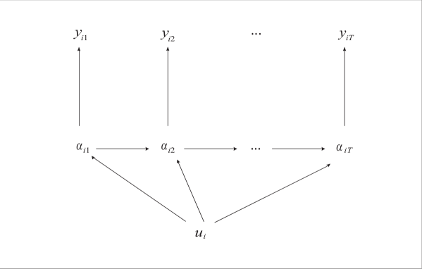
Figure 1: Path diagram of the MLAR model.

Obviously, the MLAR model generalises the LAR model. In particular, with $k=1$ the two models coincide, so that in the following they will be indifferently indicated by LAR or MLAR(1). With $k>1$, instead, the first model is expected to have a better fit to the data. This is because the mean value of every $\alpha_{it}$ and the correlation coefficient between $\alpha_{i,t-1}$ and $\alpha_{it}$ are not constant, but change according to the latent variable $u_{i}$. We stress that the latent process based on the above assumptions is still continuous, since the support of every latent variable $\alpha_{it}$ is $\Re$. In particular, we can simply realise that assumption A3 implies the following mixture model referred to the marginal distribution of each latent variable:

$$\alpha_{it}\sim\sum_{h}\phi(\alpha_{it};\xi_{h},\sigma^{2})\pi_{h},\quad i=1,\ldots,n,\>t=1,\ldots,T,$$

where $\phi(\alpha_{it};\xi_{h},\sigma^{2})$ is the density function of a Normal distribution with parameters $\xi_{h}$ and $\sigma^{2}$. Similarly, concerning the marginal distribution of $(\alpha_{i,t-1},\alpha_{it})$ we have that

$$(\alpha_{i,t-1},\alpha_{it})^{\prime}\sim\sum_{h}\phi_{2}((\alpha_{i,t-1},\alpha_{it})^{\prime};\xi_{h}\mbox{\boldmath$1$}_{2},\mbox{\boldmath$\Sigma$}_{u_{i}})\pi_{h},$$

which now involves the density function of a bivariate Normal distribution with mean $\xi_{h}\mbox{\boldmath$1$}_{2}$, where $\mbox{\boldmath$1$}_{2}$ denote a vector of two ones, and variance-covariance matrix

$$\mbox{\boldmath$\Sigma$}_{h}=\sigma^{2}\left(\begin{array}[]{cc}1&\rho_{h}\\ \rho_{h}&1\\ \end{array}\right).$$

The above arguments imply that a possible interpretation of the MLAR model may be based on considering the population of subjects, from which the observed sample comes, as made of $k$ subpopulations (or latent classes), such that a LAR model with the same parameters holds within each subpopulation. In fact, the probability mass (or density) function of the distribution of the response vector $\mbox{\boldmath$y$}_{i}$ given all the observable covariates $\mbox{\boldmath$X$}_{i}$ may be expressed as a mixture of LAR models. In particular, we have the following manifest distribution:

$$p(\mbox{\boldmath$y$}_{i}|\mbox{\boldmath$X$}_{i})=\sum_{h}p^{(h)}(\mbox{\boldmath$y$}_{i}|\mbox{\boldmath$X$}_{i})\pi_{h},$$ (13)

with $p^{(h)}(\mbox{\boldmath$y$}_{i}|\mbox{\boldmath$X$}_{i})$ defined as in (8), for $h=1,\ldots,k$. However, in order to implement the estimation method for the model parameters, it is more convenient to express this probability or density on the basis of the latent effect $\alpha_{it}^{*}$ which follows a standardised AR(1) process. Then, we have

$$p^{(h)}(\mbox{\boldmath$y$}_{i}|\mbox{\boldmath$X$}_{i}) = \int p(y_{i1}|\alpha_{i1}^{*},\mbox{\boldmath$x$}_{i1})f^{(h)}(\alpha_{i1}^{*})\int p(y_{i2}|\alpha_{i2}^{*},\mbox{\boldmath$x$}_{i2})f^{(h)}(\alpha_{i2}^{*}|\alpha_{i1}^{*})\cdots$$ (14)

$$\cdots\int p(y_{iT}|\alpha_{iT}^{*},\mbox{\boldmath$x$}_{iT})f^{(h)}(\alpha_{iT}^{*}|\alpha_{i,T-1}^{*})d\alpha_{iT}\cdots d\alpha_{i2}d\alpha_{i1},$$

where $p(y_{it}|\alpha_{it}^{*},\mbox{\boldmath$x$}_{it})$ is computed on the basis of (12) and

$$f^{(h)}(\alpha_{i1}^{*}) = \phi(\alpha_{i1}^{*};0,1),$$ (15)

$$f^{(h)}(\alpha_{it}^{*}|\alpha_{i,t-1}^{*}) = \phi(\alpha_{it}^{*};\alpha_{i,t-1}^{*}\rho_{h},1-\rho^{2}_{h}).$$ (16)

An efficient way to compute function (14) is described in Section 4.1.

However, our main aim here is not that of classifying subjects in different subpopulations, but that of having a flexible structure for the latent process. In fact, by rising $k$, we have an increasing degree of flexibility of the distribution of $\mbox{\boldmath$\alpha$}_{i}$ with respect to assuming a standard AR(1) process as in the LAR model. In fact, it is well-known that, with a suitable number of components and under suitable conditions, a mixture distribution can adequately approximate any distribution. The same principle has been exploited by Bartolucci, (2005) to propose a flexible method to classify univariate observations and by Scaccia and Bartolucci, (2005) to propose a regression model with a flexible distribution for the error terms.

In order to clarify the above point, in Figure 2 we represent the density function of the marginal distribution of every $\alpha_{it}$ and of $(\alpha_{i,t-1},\alpha_{it})$ for the LAR model and for a MLAR model with $k=2$ components and different parameter values. In particular, the top panel in Figure 2 is referred to LAR model with parameters $\rho=0.95$ and $\sigma^{2}=1.00$, the middle panel is referred to the MLAR(2) model with parameters $\xi_{1}=\xi_{2}=0.00$, $\rho_{1}=0.95$, $\rho_{2}=0.50$, $\pi_{1}=0.70$ and $\pi_{2}=0.30$, whereas the bottom panel is referred to the same MLAR(2) model with $\xi_{1}=-0.50$ and $\xi_{2}=1.00$. In order to make clear the comparison among the plots, we used the same level curves for all bivariate distributions in Figure 2 (right panels), which are defined on the basis of a grid of equispaced points on the logarithmic scale.

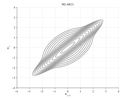
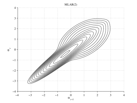
Figure 2: Density function of the univariate distribution of $\alpha_{it}$ (left) and of the bivariate distribution of $(\alpha_{i,t-1},\alpha_{it})$ (right) under the LAR model (top) with $\rho=0.95$ and $\sigma^{2}=1.00$ and under the MLAR(2) model with $\rho_{1}=0.95$, $\rho_{2}=0.50$, $\pi_{1}=0.70$, $\pi_{2}=0.30$, and $\sigma^{2}=1.00$ and with $\xi_{1}=\xi_{2}=0.00$ (middle) and $\xi_{1}=-0.50$ and $\xi_{2}=1.00$ (bottom).

We observe that with only two components, very different shapes of the density function of the latent variable distribution may be obtained. In particular, when $\xi_{1}=\xi_{2}$ (middle panel of Figure 2), both univariate and bivariate distributions are still symmetric. However, the bivariate density function has a different shape with respect to that under the LAR model, due to a much higher dispersion around the middle of the plot. Moreover, with $\xi_{1}\neq\xi_{2}$ (bottom panel), these distributions are also asymmetric, with the density of points in the North-West region of the bivariate plot that considerably rises. In a similar way we can even generate more complex shapes if we use, for instance, values of $k$ higher than 2, at the cost of a moderate increase of the number of parameters.

4 Likelihood inference

In this section, we deal with likelihood inference for the model proposed in Section 3. In particular, we first show how to efficiently compute the model log-likelihood. Then we deal with its maximisation by an EM algorithm and we describe how to compute standard errors and predict individual effects. Finally, we deal with the choice of the number of mixture components.

4.1 Computation of the model likelihood

Since the sample units are assumed to be independent, the model likelihood has logarithm

$$\ell(\mbox{\boldmath$\theta$})=\sum_{i}\log p(\mbox{\boldmath$y$}_{i}|\mbox{\boldmath$X$}_{i}),$$ (17)

where $\theta$ is a short hand notation for all the non-redundant model parameters and, for every subject $i$, $p(\mbox{\boldmath$y$}_{i}|\mbox{\boldmath$X$}_{i})$ denotes the probability mass (or density) function given in (13), seen as a function of these parameters.

In order to efficiently compute $p(\mbox{\boldmath$y$}_{i}|\mbox{\boldmath$X$}_{i})$, we exploit a recursion developed in the hidden Markov literature. First of all, we transform the series of integrals to compute $p^{(h)}(\mbox{\boldmath$y$}_{i}|\mbox{\boldmath$X$}_{i})$, which is defined in (14), in a series of sums on a suitable grid of quadrature points, as proposed by Heiss, (2008). Let $q$ denote the number of quadrature points and let $\nu_{m}$ denote the $m$-th quadrature knot, with $m=1,\ldots,q$. Moreover, for each mixture component $h$, let $\omega_{m}^{(h)}$ denote the $m$-th weight for the integral with respect to $\alpha_{i1}$ and let $\omega_{m_{1}m_{2}}^{(h)}$ denote the $m_{2}$-th weight for the integral with respect to $\alpha_{it}$, given that the $m_{1}$-th knot is selected for the integral with respect to $\alpha_{i,t-1}$. Then, the expression in (14) becomes:

$$p^{(h)}(\mbox{\boldmath$y$}_{i}|\mbox{\boldmath$X$}_{i})=\sum_{m_{1}}p(y_{i1}|\nu_{m_{1}},\mbox{\boldmath$x$}_{i1})\omega^{(h)}_{m_{1}}\sum_{m_{2}}p(y_{i2}|\nu_{m_{2}},\mbox{\boldmath$x$}_{i2})\omega^{(h)}_{m_{1}m_{2}}\cdots\sum_{m_{T}}p(y_{iT}|\nu_{m_{T}},\mbox{\boldmath$x$}_{iT})\omega^{(h)}_{m_{T-1}m_{T}}.$$ (18)

In practice, the knots are taken on a suitable grid of points between two extremes, say $-5$ and $5$, and the corresponding weights are computed as follows:

$$\omega_{m}^{(h)} = \frac{f^{(h)}(\nu_{m})}{\sum_{l}f^{(h)}(\nu_{l})},\quad m=1,\ldots,q,$$

$$\omega_{m_{1}m_{2}}^{(h)} = \frac{f^{(h)}(\nu_{m_{2}}|\nu_{m_{1}})}{\sum_{l}f^{(h)}(\nu_{m_{2}}|\nu_{l})},\quad m_{1},m_{2}=1,\ldots,q,$$ (19)

for $h=1,\ldots,k$, on the basis of the density functions defined in (15) and (16). The quadrature knots and the corresponding weights could be found by a more complex method, such as the Guass-Hermite method. However, we experienced that the above method leads to essentially equivalent solutions when $q$ is large enough.

We can easily recognise that expression (18) is the same expression of the manifest distribution of the LM model given in (9). The only difference is that for the LM model we have support points ($\xi_{h}$) and initial and transition probabilities ($\pi_{h}$, $\pi_{h_{1}h_{2}}$) to be estimated on the basis of the data. Here, we have knots ($\nu_{m}$) and weights ($\omega^{(h)}_{m}$, $\omega^{(h)}_{m_{1}m_{2}}$) which are instead given, with the exception of the weights $\omega^{(h)}_{m_{1}m_{2}}$ which only depend on the correlation coefficient $\rho_{h}$. However, the same recursion of Baum et al., (1970) may be used to efficiently compute (18), and then obtain $p^{(h)}(\mbox{\boldmath$y$}_{i}|\mbox{\boldmath$X$}_{i})$ from which we obtain $p(\mbox{\boldmath$y$}_{i}|\mbox{\boldmath$X$}_{i})$ by (13) and the log-likelihood $\ell(\mbox{\boldmath$\theta$})$ by (17). Note that applying the recursion at issue is essentially equivalent to apply the SGQ of Heiss, (2008) and to the method of Bartolucci and De Luca, (2001, 2003) to compute the likelihood function of SV models.

4.2 Maximum likelihood estimation

As derived above, once a suitable set of quadrature knots has been adopted, the likelihood of the proposed model may be seen as equivalent to that of an LM model with covariates and latent parameters suitably constrained. Then, maximum likelihood (ML) estimation may be performed by an adaptation of the EM algorithm for the LM model described by Bartolucci and Farcomeni, (2009); see also Baum et al., (1970) and Dempster et al., (1977). In the following, we outline this extended algorithm, referring for some details to Bartolucci and Farcomeni, (2009).

The EM algorithm is based on the so-called complete data log-likelihood that, in the present case, corresponds to the log-likelihood that we could compute if we knew, for $i=1,\ldots,n$, the value of the latent variable $u_{i}$ and the value of the quadrature knot for $\alpha_{it}$, $t=1,\ldots,T$. This is equivalent to the knowledge of the dummy variables $w_{ih}$, $i=1,\ldots,n$, $h=1,\ldots,k$, and $z_{imt}$, $i=1,\ldots,n$, $m=1,\ldots,q$, $t=1,\ldots,T$, where $w_{ih}=I\{u_{i}=h\}$ and $z_{imt}=I\{\alpha_{it}=\nu_{m}\}$. Up to a constant term, the complete data log-likelihood may be expressed as

$$\ell^{*}(\mbox{\boldmath$\theta$})=\sum_{i}\sum_{h}w_{ih}\left\{\log\pi_{h}+\sum_{m_{1}}\sum_{m_{2}}\sum_{t>1}z^{*}_{im_{1}m_{2}t}\log\omega^{(h)}_{m_{1}m_{2}}+\sum_{m}\sum_{t}z_{imt}\log p(y_{it}|\nu_{m},\mbox{\boldmath$x$}_{it})\right\},$$ (20)

where $z^{*}_{im_{1}m_{2}t}=z_{im_{1},t-1}z_{im_{2}t}$.

The EM algorithm alternates the following steps until convergence:

• E-step: compute the conditional expected value of the complete data log-likelihood given the observed data and the current estimate of $\theta$;

• M-step: maximise the expected value above with respect to $\theta$.

The E-step is equivalent to computing the conditional expected value, given the observed data, of every dummy variable $w_{ih}$ and of the products $w_{ih}z_{imt}$ and $w_{ih}z_{im_{1}m_{2}t}^{*}$. In practice, for $i=1,\ldots,n$, we have that

$$\hat{w}_{ih}=E(w_{ih}|data)=\frac{p^{(h)}(\mbox{\boldmath$y$}_{i}|\mbox{\boldmath$X$}_{i})}{p(\mbox{\boldmath$y$}_{i}|\mbox{\boldmath$X$}_{i})},\quad h=1,\ldots,k,$$

where the probabilities are computed on the basis of the current value of the parameters and data stands for “observed data”. Moreover, we have that

$$\widehat{(w_{ih}z_{imt})}=E(w_{ih}z_{imt}|data)=\hat{w}_{ih}E(z_{imt}|w_{ih}=1,data),\quad m=1,\ldots,q,\>t=1,\ldots,T,$$

where $E(z_{imt}|w_{ih}=1,data)$ is the posterior probability that subject $i$ is in state $h$ at time occasion $t$ given that $u_{i}=h$, and

$$\widehat{(w_{ih}z^{*}_{im_{1}m_{2}t})}=E(w_{ih}z^{*}_{im_{1}m_{2}t}|data)=\hat{w}_{ih}E(z^{*}_{im_{1}m_{2}t}|w_{ih}=1,data),\quad m_{1},m_{2}=1,\ldots,q,\>t=2,\ldots,T,$$

where $E(z^{*}_{im_{1}m_{2}t}|w_{ih}=1,data)$ is the posterior probability that subject $i$ moves from state $m_{1}$ to state $m_{2}$ at occasion $t$, given that $u_{i}=h$. These posterior probabilities may be computed by suitable recursions; see Baum et al., (1970), Bartolucci and Farcomeni, (2009), and Bartolucci et al., (2010) for details.

Once the expected values of the dummy variables have been substituted in (20), the resulting function is maximised with respect to the model parameters, which are consequently updated. The easiest parameters to update are the probabilities $\pi_{h}$, for which we have an explicit solution

$$\pi_{h}=\frac{\sum_{i}\hat{w}_{hi}}{\sum_{l}\sum_{i}\hat{w}_{li}},\quad h=1,\ldots,k.$$

Then, in order to update each parameter $\rho_{h}$, $h=1,\ldots,k$, we have to maximise, by a numerical optimisation algorithm, the function

$$\sum_{i}\sum_{m_{1}}\sum_{m_{2}}\sum_{t>1}\widehat{(w_{ih}z^{*}_{im_{1}m_{2}t})}\log\omega^{(h)}_{m_{1}m_{2}},$$

which depends on this parameter through (19). Finally, the other model parameters, that is $\xi_{1},\ldots,\xi_{k}$, $\beta$, and $\sigma^{2}$, are update by maximising the function

$$\sum_{i}\sum_{h}\sum_{m}\sum_{t}\widehat{(w_{ih}z_{imt})}\log p(y_{it}|\nu_{m},\mbox{\boldmath$x$}_{it}),$$

which depends on these parameters through (12). This maximisation may be performed by a NR iterative algorithm, the implementation of which is not difficult, due to the availability of explicit expressions for the first and second derivatives of the target function.

Since the EM algorithm is rather slow to converge, after a certain number of steps we switch to a full NR algorithm to maximise the model log-likelihood $\ell(\mbox{\boldmath$\theta$})$. This algorithm updates the model parameters $\theta$ by adding the following quantity $\mbox{\boldmath$J$}(\mbox{\boldmath$\theta$})^{-1}\mbox{\boldmath$s$}(\mbox{\boldmath$\theta$})$, where $\mbox{\boldmath$s$}(\mbox{\boldmath$\theta$})$ denotes the score vector for $\ell(\mbox{\boldmath$\theta$})$ and $\mbox{\boldmath$J$}(\mbox{\boldmath$\theta$})$ denotes the corresponding observed information matrix. The latter is equal to minus the second derivative of $\ell(\mbox{\boldmath$\theta$})$ with respect to $\theta$. Following Bartolucci and Farcomeni, (2009), the score vector is computed as the first derivative of the expected value of complete data log-likelihood, which is obtained after an E-step. The observed information matrix is then obtained on the basis of the numerical derivative of $\mbox{\boldmath$s$}(\mbox{\boldmath$\theta$})$.

We take the value of $\theta$ at convergence of the NR algorithm as the ML estimate $\hat{\mbox{\boldmath$\theta$}}$. As it typically happens for latent variable models, the model likelihood may be multimodal and the point at convergence depends on the starting values for the parameters, which need to be carefully chosen. Then, we suggest to try different starting values in order to be sure that the found solution corresponds to the global maximum of $\ell(\mbox{\boldmath$\theta$})$.

Once the ML estimates have been computed, it may be of interest to obtain the corresponding standard errors. These may be obtained in the usual way on the basis of $\mbox{\boldmath$J$}(\hat{\mbox{\boldmath$\theta$}})^{-1}$ and may be used to compute confidence intervals for the parameters and perform Wald testing about certain hypotheses of interest. More generally, hypotheses of interest may be tested by a likelihood ratio statistic that, under the usual regularity conditions, has asymptotic distribution of $\chi^{2}$-type.

On the basis of the parameter estimates it may also be of interest to predict every latent variable $\alpha_{it}$. This may be performed through the following posterior expected value given the observed data:

$$\hat{\alpha}_{it}=\sum_{h}\sum_{m}\widehat{(w_{ih}z_{imt})}(\hat{\xi}_{h}+\nu_{m}\hat{\sigma}),\quad i=1,\ldots,n,\>t=1,\ldots,T,$$ (21)

with all quantities computed on the basis of the final estimate $\hat{\mbox{\boldmath$\theta$}}$.

For the case of binary and ordinal response variables, we implemented the above strategy to obtain the ML estimate of $\theta$, which is based on the joint use of an EM and of an NR algorithm, in a series of Matlab functions that we make available to the reader upon request. In our experience, this strategy properly works and provides ML estimates and corresponding standard errors in a reasonable amount of time, provided that $k$ is not too large.

4.3 Selection of the number of mixture components and of quadrature points

In applying the proposed model, of crucial importance is the choice of the number of mixture components ($k$) and of quadrature points ($q$). Regarding the choice of $q$, we have to use a value which is large enough to guarantee an adequate approximation of the true likelihood function, that is the likelihood that we could obtain by exactly computing the multiple integral in (14). At this regard, the strategy we suggest is based on trying, for a given $k$, increasing values of $q$ until the maximum of $\ell(\mbox{\boldmath$\theta$})$ does not significantly change with respect to the previous value of $q$. In our application, for instance, we start with $q=21$ and we increase the value of $q$ by 10 at each attempt, stopping when the maximum of $\ell(\mbox{\boldmath$\theta$})$ increases less than $10^{-3}$.

Through the above strategy, we find a suitable value of $q$ for a given $k$. The point now is how to choose $k$. In summary, the strategy we suggest consists of increasing $k$ until the estimated latent structure does not significantly change. In practice, for each tried value of $k$ we obtain the predicted latent variables $\alpha_{it}$ through (21) on the basis of $\hat{\mbox{\boldmath$\theta$}}$ and, for $k>1$, we compute the correlation index between these predicted values and those computed with $k-1$ mixture components. The first value of $k$ such that this correlation index is higher than a suitable threshold (we use 0.99 in our application) is taken as the optimal number of mixture components.

Note that, in order to select $k$, we could also rely on information criterion such as the Akaike Information Criterion (Akaike,, 1973) or the Bayesian Information Criterion (Schwarz,, 1978). However, we experimented in our applications that these criteria tend to choose a value of $k$ higher than necessary, whereas we have evidence that the criterion suggested above, which is based on direct assessment of the estimated latent structure, has good performance.

5 Application to Self-reported health status

To illustrate the proposed approach, we consider a dataset which derives from the Health and Retirement Study conducted by the University of Michigan (see http://www.rand.org/labor/aging/dataprod for detailed illustration). After a description of the dataset, we report the results of its analysis based on the proposed approach.

5.1 Dataset description

The dataset is referred to a sample of $n=7,074$ American individuals who were asked to express opinions on their health status at $T=8$ approximately equally spaced occasions, from 1992 to 2006. The response variable (self-reported health status) is measured on a scale based on five ordered categories: “poor”, “fair”, “good”, “very good”, and “excellent”. For every subject some covariates are also available: gender, race, education, and age (at each time occasion). Table 1 shows some descriptive statistics about these covariates, whereas Table 2 shows the marginal distribution of the response variable over the 8 occasions of interview.

Variable	Category	$\%$	Mean	St.Dev.
gender:	female	58.1	–	–
	male	41.9	–	–
race:	white	82.9	–	–
	non white	17.1	–	–
education:	high school	60.9	–	–
	some college	19.7	–	–
	college and above	19.4	–	–
age (in 1992):		–	54.8	5.5

Table 1: Distribution of the covariates.

	occasion of interview
SRH category	1	2	3	4	5	6	7	8	Total
poor	4.7	4.7	4.7	6.1	5.5	5.9	7.2	8.1	5.9
fair	11.5	13.0	13.1	17.0	15.6	16.9	19.2	20.3	15.8
good	27.2	28.9	28.1	32.0	30.6	32.0	32.2	32.0	30.4
very good	30.8	32.6	34.3	31.1	33.6	32.3	30.0	29.7	31.8
excellent	25.7	20.8	19.8	13.7	14.7	13.0	11.4	10.0	16.1
Total	100.0	100.0	100.0	100.0	100.0	100.0	100.0	100.0	100.0

Table 2: Distribution of the response variable over the occasions of interview in terms of percentage frequencies.

As shown in Table 1, the main part of individuals in the sample are females ($58.1\%$) and whites ($82.9\%$), with an average age at the first time occasion equal to $54.8$; we recall that the occasions of interview are around two years far apart. The $60.9\%$ of the sample has a high-school diploma, whereas a college degree or a higher title is possessed by the $19.4\%$ of subjects. In the following, the covariate education is introduced in the model by assigning increasing scores to its categories: 1 for “high school”, 2 for “some college” (i.e., a high school or a general education diploma and more than 12 years of education), 3 for “college and above” (i.e., a college degree, such as Bachelor of Arts, or an higher title, such as PhD).

About the distribution of the response variable at each time occasion (see Table 2), we observe that more than the $60\%$ of responses is equally distributed between categories “good” and “very good”, being substantially stable over time. Moreover, the $16.1\%$ of individuals evaluates the health status as “excellent”, with a decreasing trend (the percentage is over $25.7\%$ at the first occasion and it decreases to $10.0\%$ at the eighth one). On the other side, the remaining part of individuals gives a negative judgement to the health status, with increasing percentages over time: from $4.7\%$ to $8.1\%$ and from $11.5\%$ to $20.3\%$ for categories “poor” and “fair” response, respectively.

More insights about the subjects’ responses to the questionnaire may be derived on the basis of the empirical transition matrix reported in Table 3. Each row of this matrix shows the percentage frequencies of the five response categories at occasion $t$ given the response at occasion $t-1$, with $t=2,\ldots,T$.

	SRH at $t$
SRH at $t-1$	poor	fair	good	very good	excellent	Total
poor	54.5	34.1	8.4	2.5	0.7	100.0
fair	12.8	51.0	27.4	7.2	1.6	100.0
good	2.5	16.5	53.3	23.6	4.1	100.0
very good	0.8	4.7	25.9	55.6	13.0	100.0
excellent	0.4	1.9	10.6	33.7	53.4	100.0

Table 3: Conditional empirical distributions of the response variable at time $t$ given the response at time $t-1$, with $t=2,\ldots,T$ (percentage frequencies).

In general, a rather high persistence of the judgement about the health status results, since more than one half of responses at time $t$ is in the same category as the response at time $t-1$, and percentages included between $12.8\%$ and $34.0\%$ lie in an adjacent category. On the other hand, jumps between different and not adjacent response categories in consecutive time occasions are observable for the remaining part of the sample. For example, among subjects who evaluate their health status as “poor” at a given occasion, the $8.4\%$ evaluates it as “good” at the next occasion; on the contrary, among subjects who respond “very good” at a given occasion, only the $4.7\%$ responds “fair” at the following occasion.

5.2 Model selection

To the data described above, we preliminary fit the proposed MLAR model for different values of $k$ (number of mixture components) and $q$ (number of quadrature points). To take into account the ordinal nature of the response variable, the model is formulated on the basis of the global logit parameterisation defined in equation (11). Then, the optimal values of $k$ and $q$ is chosen as described in Section 4.3. We recall that, as concerns the selection of $q$ (given $k$) the adopted procedure starts from $q=21$ and increases it by 10; the number of quadrature points is selected in correspondence of the first difference between two consecutive maximum log-likelihood values smaller than 0.001. With reference to the selection of $k$, the adopted strategy consists of computing the correlation index $\rho_{k-1,k}$ between the predicted $\alpha_{it}$ values of MLAR($k$) and those of MLAR($k-1$), for increasing values of $k$ starting from 2. When $\rho_{k-1,k}$ is greater than 0.99, $k$ is not raised anymore and its last value is taken as the optimal number of mixture components. Table 4 reports the main results of this model selection procedure.

	$k=1$		$k=2$		$k=3$
$q$	log-likelihood	difference	log-likelihood	difference	log-likelihood	difference
21	-63609.195	–	-62978.009	–	-62831.584	–
31	-63624.648	-15.453	-62996.639	-18.630	-62844.763	-13.179
41	-63624.657	-0.009	-62998.591	-1.952	-62845.683	-0.920
51	-63624.657	0.000	-62998.613	-0.022	-62845.688	-0.005
61	-63624.657	0.000	-62998.613	0.000	-62845.688	0.000
71	-63624.657	0.000	-62998.613	0.000	-62845.688	0.000
81	-63624.658	0.000	-62998.614	0.000	-62845.688	0.000
91	-63624.658	0.000	-62998.614	0.000	-62845.688	0.000
101	-63624.658	0.000	-62998.614	0.000	-62845.688	0.000
		$\rho_{12}=0.9783$		$\rho_{23}=0.9974$

Table 4: Log-likelihoods and differences between consecutive values for $k=1,2,3$ and $q$ from $21$ to $101$ with step 10; $\rho_{k-1,k}$ is the correlation index between predicted values of $\alpha_{it}$ under model MLAR($k-1$) and model MLAR($k$); in boldface are the differences between maximum values of consecutive log-likelihoods which are smaller than 0.001 for the first time.

On the basis of the results in Table 4, we conclude that the adequate number of quadrature points ($q$) is equal to $51$ for $k=1$ and to $61$ for $k=2$ and $k=3$. For illustrative purposes, in the table we also show results until $q=101$. Indeed, we observe that increasing $q$ over the selected value is unnecessary, as the corresponding values of the maximum log-likelihood become stable. Moreover, being $\rho_{12}$ smaller than 0.99 and $\rho_{23}$ equal to 0.9974, we choose $k=3$ mixture components. As mentioned at the end of Section 4.3, we note that the proposed selection criterion for $k$ leads to selecting a more parsimonious model with respect to that selected by BIC. Indeed, in this last case we obtain decreasing values of the BIC index at least until $k=4$. Moreover, in our application this criterion becomes soon hardly to apply, as for $k\geq 4$ the log-likelihood becomes rather flat and, therefore, estimates result highly unstable.

To evaluate the goodness-of-fit of the selected model, we compare it with the MLAR(1) (or LAR) model and the MLAR(2) model. We also compare these models with the LM model with covariates and initial distribution of the Markov chain equal to the stationary distribution. For a given number of latent states $k$, the last model is indicated by LM($k$); it is fitted for $k=1,\ldots,10$. The results of this comparison in terms of maximum log-likelihood and BIC index are reported in Table 5.

	LM($k$)			MLAR($k$)
$k$	log-likel.	# param.	BIC	log-likel.	# param.	BIC
1	-80,792	8	161,650	-63,625	10	127,340
2	-69,866	11	139,830	-62,999	13	126,110
3	-65,815	16	131,770	-62,846	16	125,830
4	-64,007	23	128,220	–	–	–
5	-63,370	32	127,020	–	–	–
6	-63,098	43	126,580	–	–	–
7	-63,020	56	126,540	–	–	–
8	-62,852	71	126,330	–	–	–
9	-62,782	88	126,340	–	–	–
10	-62,617	107	126,180	–	–	–

Table 5: Log-likelihood, number of parameters, and BIC index for the LM($k$) model, with $k=1,\ldots,10$, and the MLAR($k$) model, with $k=1,2,3$.

From Table 5 we conclude that the smallest BIC index is for the MLAR(3) model, to which correspond a maximum log-likelihood of -62,846 with 16 parameters. To obtain a higher log-likelihood with the LM model, we need at least $k=9$ latent states and, consequently, at least 88 parameters. This confirms that the proposed model reaches levels of goodness-of-fit comparable with those of the LM model but, at the same time, a level of parsimony close to that of the LAR model, since only 6 parameters are added to this model. However, in comparing the MLAR model with the LM model we have to consider that, especially for large values of $k$, the likelihood of the second presents several local maxima. Therefore, it is not ensured that the reported values of the log-likelihood for this model corresponds to global maxima. On the other hand, at least for this application, we did not find evidence of more local maxima of the MLAR model log-likelihood. This is reasonable because of the reduced number of parameters.

5.3 Parameter estimates and prediction of latent effects

The estimates of the parameters of most interest of the selected model and of comparable models are reported in Tables 6 and 7. We recall the we selected model MLAR(3). In particular, for models MLAR(1) (or LAR), MLAR(2), and MLAR(3), Table 6 reports the estimates of the cutpoints and of the regression coefficients entering equation (4) together with the corresponding standard errors. Moreover, Table 7 reports the estimates of the parameters on which the latent structure depends.

	MLAR(1)	MLAR(2)	MLAR(3)
$\hat{\mu}_{1}$	7.0155	8.2661	8.9678
$\hat{\mu}_{2}$	3.8670	4.5033	4.8351
$\hat{\mu}_{3}$	0.6607	0.6173	0.7006
$\hat{\mu}_{4}$	-2.7646	-3.5160	-3.7157
$\hat{\beta}_{1}$ (female)	-0.2056	-0.2148	-0.2317
	(0.0738)	(0.0890)	(0.0958)
$\hat{\beta}_{2}$ non white	-1.5175	-1.6884	-1.9735
	(0.0968)	(0.1149)	(0.1266)
$\hat{\beta}_{3}$ education	1.8182	2.2052	2.3846
	(0.0755)	(0.0936)	(0.1020)
$\hat{\beta}_{4}$ age	-0.1085	-0.1197	-0.1299
	(0.0028)	(0.0033)	(0.0036)

Table 6: Fixed part estimates from fitting model MLAR($k$), $k=1,2,3$; in brackets are the standard errors for the regression coefficients.

$k$	$h$	$\hat{\xi}_{h}$	$\hat{\rho}_{h}$	$\hat{\pi}_{h}$	$\hat{\sigma}^{2}$
1	1	0.0000	0.9529	1.0000	9.8151
2	1	-0.1073	0.9788	0.7634	16.5169
2	2	0.3461	0.5584	0.2366	16.5169
3	1	-2.6400	0.5204	0.1399	17.0247
3	2	-0.0578	0.9761	0.7146	17.0247
3	3	2.8237	0.3472	0.1455	17.0247

Table 7: Estimates of the parameters affecting the latent process distribution under model MLAR($k$), $k=1,2,3$.

From Table 6 we observe that the estimated cutpoints $\hat{\mu}_{1},\ldots,\hat{\mu}_{4}$ are ordered as we may expect in accordance with the parameterisation defined by (11). Moreover, on the basis of the $t$-statistics that may be computed for the regression coefficients, we conclude that all covariates are significant under every model considered in the table. However, the magnitude of each point estimate increases (in absolute value) as $k$ goes from 1 to 3, while retaining the same sign. For instance, the effect of education increases from 1.8182 to 2.3846. Less evident is the variation of effect of gender (female with respect to male), which changes from -0.2056 to -0.2317.

The results in Table 7 imply that the estimated latent structure is rather different under models MLAR(1), MLAR(2), and MLAR(3). While under the MLAR(1) model all subjects are concentrated in only one class characterised by a very high correlation ($\hat{\rho}_{1}=0.9529$), the situation is more complex under the other two models. With the MLAR(2) only the $76.34\%$ of subjects belong to a class with a high correlation ($\hat{\rho}_{1}=0.9788$), whereas for the remaining $23.66\%$ the correlation estimate is located to a positive intermediate level ($\hat{\rho}_{2}=0.5584$), being the estimate of support point higher in this latter class ($\hat{\xi}_{2}=0.3461$ versus $\hat{\xi}_{1}=-0.1073$). Under the MLAR(3) model, we observe one class, including the $71.46\%$ of subjects, very similar to that detected under the MLAR(1) model, being the correlation coefficient equal to 0.9761 and the corresponding support point very close to 0. Then, the remaining part of subjects results equally distributed between the other two classes, that show opposite values of the support points ($\hat{\xi}_{1}=-2.6400$ and $\hat{\xi}_{3}=2.8237$) and intermediate levels of correlation. Mostly for subjects in class 3 the correlation between individual effects in consecutive occasions is rather weak ($\hat{\rho}_{3}=0.3472$), so that we may suppose that these subjects are characterised by sudden changes in unobservable factors affecting their health status.

The above results are well illustrated by the density functions of the univariate distribution of the individual effects $\alpha_{it}$ and of the bivariate distribution of $(\alpha_{i,t-1},\alpha_{it})$ represented in Figure 3. Indeed, while in the MLAR(1) model values at time $t$ are highly correlated to values at time $t-1$, under the MLAR(2) model and, more evidently under MLAR(3) model, a higher dispersion of the individual effects $\alpha_{it}$ is observed on the bivariate plot. On the other hand, the univariate distributions does not seem to deviate from normality under both MLAR(2) and MLAR(3) models.

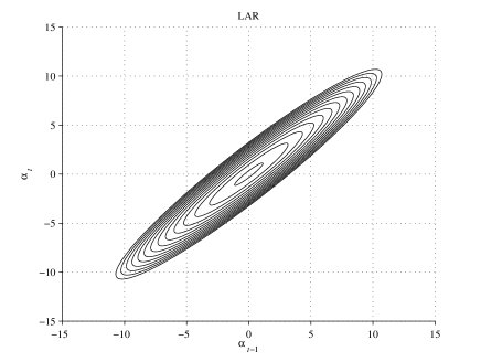
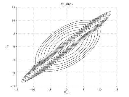
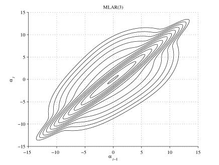
Figure 3: Estimated density function of the univariate distribution of $\alpha_{it}$ (left) and of the bivariate distribution of $(\alpha_{i,t-1},\alpha_{it})$ (right) under the LAR model (top), the MLAR(2) model (middle), and the MLAR(3) model (bottom).

Another way to compare the estimated latent structure under the different models here considered is through the predicted $\alpha_{it}$, as computed by (21), rather than through the a priori distributions in the previous Figure. These predicted values are represented, also for the same LM(10) model already considered in Section 5.2, in Figure 4. In particular, each plot in the figure represents points with coordinates ($\hat{\alpha}_{i,t-1},\hat{\alpha}_{it}$), for $i=1,\ldots,n$ and $t=2,\ldots,T$.

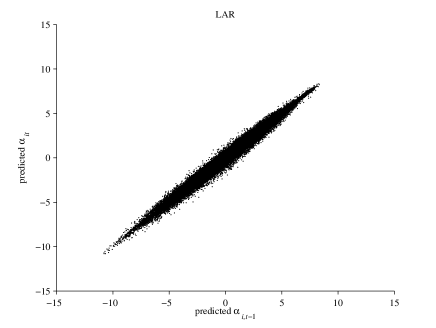
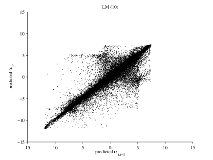
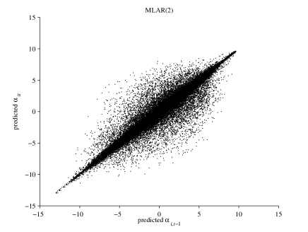
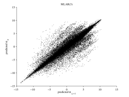
Figure 4: Predicted values of $(\alpha_{i,t-1},\alpha_{it})$, $i=1,\ldots,n$, $t=2,\ldots,T$, under the LAR model (top left), the LM model (top right), the MLAR(2) model (bottom left), and the MLAR(3) model (bottom right).

According to the plots in Figure 4, under models MLAR(2), MLAR(3), and LM(10) there is a stronger dispersion of the predicted values with respect to the LAR model. In particular, the difference of the plot obtained under the selected MLAR(3) model is neat with respect to the plot obtained under the LAR model, whereas it is less evident with respect to the plot obtained under the LM(10) model, which however uses much more parameters. In practice, it seems that the proposed model allows for more erratic trends of the unobserved individual effects across time with respect to the LAR model. This is a direct consequence of the greater flexibility of the MLAR model, which is obtained at the cost of a reduced number of additive parameters.

6 Discussion

In this paper, we extend the Latent Autoregressive (LAR) model for longitudinal data (Chi and Reinsel,, 1989; Heiss,, 2008), by adopting a latent structure for the unobserved heterogeneity which is based on a mixture of AR(1) processes with specific mean values and correlation coefficients, but with common variance. The proposed model, named Mixture Latent Autoregressive (MLAR) model, is formulated in a general way, so that it may be easily adapted to different types of response variable (binary, ordinal, or continuous). It is important to note that, as for the LAR model, the latent process on which the proposed model is based is continuous.

Compared to the latent Markov (LM) model with covariates in which the latent process is discrete (see Bartolucci et al., (2010) for a review), the MLAR model has some interpretative advantages, being usually more natural to consider the effect of unobservable factors or covariates as continuous rather than discrete. Moreover, the main advantage of MLAR model with respect to LAR model is the improvement of the goodness-of-fit which becomes close to that of an LM model with covariates, allowing us to adequately take into account more erratic trends in the unobservable individual effects. At the same time, the parsimony of the proposed model is kept near to that of a LAR model, avoiding the explosion of the number of parameters of the LM model when the number of latent states increases.

In order to make inference on the proposed model, we show how its likelihood may be efficiently computed by exploiting some recursions developed in the context of Hidden Markov (HM) models (Baum et al.,, 1970; MacDonald and Zucchini,, 1997). The resulting computational method is equivalent to the Sequential Gaussian Quadrature method proposed by Heiss, (2008) for the LAR model. Moreover, since the model likelihood is the same as that of an LM model with suitable constraints, then maximum likelihood estimation of the model parameters may be performed on the basis of an EM algorithm for LM models, adapting that implemented by Bartolucci and Farcomeni, (2009). To make faster the estimation, after a certain number of EM steps we suggest to switch to a Newton-Raphson algorithm, which is based on the observed information matrix obtained by a numerical method.

After parameters estimation, standard errors are obtained from the observed information matrix. Moreover, on the basis of the parameter estimates it is also possible to predict individual effects for every subject and time occasion. We show how these predicted values may be used to implement a model selection strategy for the number of mixture components of the MLAR model; we recall that each component corresponds to a separate AR(1) latent process. In particular, the number of mixture components is increased until the predicted values of the latent variable do not significantly change. This selection strategy leads us to selecting more parsimonious models with respect to alternative methods, such as those based on information criteria.

The advantages of the MLAR model with respect to the LAR model are illustrated through an application to a longitudinal dataset, coming from the Health and Retirement Study conducted by the University of Michigan, about self-evaluation of the health status. The results show evidence of three mixture components corresponding to the same number of AR(1) processes. Each component has its own specific correlation parameter. In this way, we take into account the latent trends and jumps from time to time in a more flexible way in comparison with the LAR approach. Moreover, the goodness-of-fit of the MLAR model is comparable to that of an LM model with covariates, being, at the same time, the number of parameters strongly smaller. In addition, we observe that the proposed model does not suffer from the problem of multimodal likelihood as the LM model with covariates does. This is rather obvious considering the reduced number of parameters of the first with respect to the second.

A final point concerns possible extensions of the proposed approach. A natural extension consists of generalising our model to AR processes of order two (or higher), so as to take also into account more sophisticated dependence structures. This extension may be performed along the same lines as in Bartolucci and Solis-Trapala, (2010), although we think that likelihood inference becomes more problematic, especially in terms of computational capability required to obtain maximum likelihood estimates.

Finally, the reader may wonder about a possible extension of the proposed approach in which subjects may move between different mixture components or, in equivalent terms, in which we have switching parameters for the individual AR(1) latent processes. This amounts to combine a latent AR(1) process with a latent Markov chain. We recall that in the MLAR model the latent process parameters are kept constant across time, although these parameters may be different among subjects. The extended formulation based on combining a latent AR(1) process and a latent Markov chain has been experimented by the same authors, see Bacci et al., (2010); however, they observed that the major complexity of the resulting model tends to produce estimates that are highly unstable and are rather difficult to interpret. Moreover, the goodness-of-fit reached under this extended formulation is comparable to that of the MLAR model here proposed with the same number of parameters. For these reasons we consider this model as the right compromise between making more flexible the LAR model and keeping a parsimonious structure, while retaining a continuous latent process approach.

References

- Akaike, (1973) Akaike, H. (1973). Information theory and an extension of the maximum likelihood principle. In Petrov, B. N. and Csaki, F., editors, Second International symposium of information theory, pages 267–281, Budapest. Akademiai Kiado.
- Bacci et al., (2010) Bacci, S., Bartolucci, F., and Pennoni, F. (2010). Markov-switching autoregressive latent variable models for longitudinal data. In Bowman, A., editor, Proceedings of 25th International Workshop on Statistical Modelling (IWSM 2010), University of Glasgow 5-9th July 2010, pages 79–84.
- Bandeen-Roche et al., (1997) Bandeen-Roche, K., Miglioretti, D. L., Zeger, S. L., and Rathouz, P. (1997). Latent variable regression for multiple discrete outcomes. Journal of the American Statistical Association, 92:1375–1386.
- Bartolucci, (2005) Bartolucci, F. (2005). Clustering univariate observations via mixtures of unimodal normal mixtures. Journal of Classification, 22:203–219.
- Bartolucci, (2006) Bartolucci, F. (2006). Likelihood inference for a class of latent Markov models under linear hypotheses on the transition probabilities. Journal of the Royal Statistical Society, series B, 68:155–178.
- Bartolucci and De Luca, (2001) Bartolucci, F. and De Luca, G. (2001). Maximum likelihood estimation for a latent variable time series model. Applied Stochastic Models for Business and Industry, 17:5–17.
- Bartolucci and De Luca, (2003) Bartolucci, F. and De Luca, G. (2003). Likelihood-based inference for asymmetric stochastic volatility models. Computational Statistical and Data Analysis, 42:445–449.
- Bartolucci and Farcomeni, (2009) Bartolucci, F. and Farcomeni, A. (2009). A multivariate extension of the dynamic logit model for longitudinal data based on a latent Markov heterogeneity structure. Journal of the American Statistical Association, 104:816–831.
- Bartolucci et al., (2010) Bartolucci, F., Farcomeni, A., and Pennoni, F. (2010). An overview of latent Markov models for longitudinal categorical data. arXiv:1003.2804.
- Bartolucci and Solis-Trapala, (2010) Bartolucci, F. and Solis-Trapala, I. (2010). Multidimensional latent markov models in a developmental study of inhibitory control and attentional flexibility in early childhood. Psychometrika, 75:725–743.
- Baum et al., (1970) Baum, L., Petrie, T., Soules, G., and Weiss, N. (1970). A maximization technique occurring in the statistical analysis of probabilistic functions of markov chains. Annals of Mathematical Statistics, 41:164–171.
- Cai, (1994) Cai, J. (1994). A Markov model of switching-regime ARCH. Journal of Business and Economic Statistics, 12:309–316.
- Chi and Reinsel, (1989) Chi, E. and Reinsel, G. (1989). Models for longitudinal data with random effects and AR(1) errors. Journal of the American Statistical Association, 84:452–459.
- Dempster et al., (1977) Dempster, A. P., Laird, N. M., and Rubin, D. B. (1977). Maximum likelihood from incomplete data via the EM algorithm (with discussion). Journal of the Royal Statistical Society, Series B, 39:1–38.
- Frühwirth-Schnatter, (2006) Frühwirth-Schnatter, S. (2006). Finite Mixture and Markov Switching Models. Springer-Verlag, United States of America.
- Goldstein, (2003) Goldstein, H. (2003). Multilevel Statistical Models. Arnold, London.
- Goodman, (1974) Goodman, L. A. (1974). Exploratory latent structure analysis using both identifiable and unidentifiable models. Biometrika, 61:215–231.
- Hagenaars and McCutcheon, (2002) Hagenaars, J. and McCutcheon, A. L. (2002). Applied Latent Class Analysis. Cambridge University Press, Cambridge, MA.
- Hambleton and Swaminathan, (1985) Hambleton, R. K. and Swaminathan, H. (1985). Item Response Theory: Principles and Applications. Kluwer Nijhoff, Boston.
- Hamilton and Susmel, (1994) Hamilton, J. D. and Susmel, R. (1994). Autoregressive conditional heteroschedasticity and changes in regime. Journal of Econometrics, 64:307–333.
- Hancock and Samuelson, (2008) Hancock, G. R. and Samuelson, K. M. (2008). Advances in Latent Variable Mixture Models. Charlotte, NC: Information Age Publishing, United States of America.
- Heiss, (2008) Heiss, F. (2008). Sequential numerical integration in nonlinear state space models for microeconometric panel data. Journal of Applied Econometrics, 23:373–389.
- Huang and Bandeen-Roche, (2004) Huang, G. and Bandeen-Roche, K. (2004). Building an identifiable latent class model, with covariate effects on underlying and measured variables. Psychometrika, 69:5–32.
- Kitagawa, (1987) Kitagawa, G. (1987). Non-gaussian state-space modeling of nonstationary time series (with discussion). Journal of the American Statistical Association, 82:1032–1063.
- Lazarsfeld, (1950) Lazarsfeld, P. F. (1950). The logical and mathematical foundation of latent structure analysis. In S. A. Stouffer, L. Guttman, E. A. S., editor, Measurement and Prediction, New York. Princeton University Press.
- Lazarsfeld and Henry, (1968) Lazarsfeld, P. F. and Henry, N. W. (1968). Latent Structure Analysis. Houghton Mifflin, Boston.
- Lindsay et al., (1991) Lindsay, B., Clogg, C., and Greco, J. (1991). Semiparametric estimation in the rasch model and related exponential response models, including a simple latent class model for item analysis. Journal of the American Statistical Association, 86:96–107.
- MacDonald and Zucchini, (1997) MacDonald, I. and Zucchini, W. (1997). Hidden Markov and other models for Discrete-Valued Time Series. Chapman & Hall, London.
- McCullagh, (1980) McCullagh, P. (1980). Regression models for ordinal data (with discussion). Journal of the Royal Statistical Society, Series B, 42:109–142.
- McCulloch and Searle, (2001) McCulloch, C. and Searle, S. (2001). Generalized, Linear, and Mixed Models. Wiley, New York.
- Quandt, (1972) Quandt, R. (1972). A new approach to estimating switching regressions. Journal of the American Statistical Society, 67:306–310.
- Quandt and Ramsey, (1978) Quandt, R. and Ramsey, J. (1978). Estimating mixtures of normal distributions and switching regressions (with discussion). Journal of the American Statistical Society, 73:730–752.
- Rossi and Gallo, (2006) Rossi, A. and Gallo, G. M. (2006). Volatility estimation via hidden Markov models. Journal of Empirical Finance, 13:203–230.
- Scaccia and Bartolucci, (2005) Scaccia, L. and Bartolucci, F. (2005). A hierarchical mixture model for gene expression data. In Vichi, M., Monari, P., Mignani, S., and Montanari, A., editors, New Developments in Classification and Data Analysis, pages 267–274. Springer.
- Schwarz, (1978) Schwarz, G. (1978). Estimating the dimension of a model. Annals of Statistics, 6:461–464.
- Shephard, (1996) Shephard, N. (1996). Statistical aspects of arch and stochastic volatility. In D. R. Cox, D. V. Hinkley, O. E. B.-N., editor, Time Series Models: In Econometric, Finance and Other fields, pages 1–67. London: Chapman & Hall.
- Skrondal and Rabe-Hesketh, (2004) Skrondal, A. and Rabe-Hesketh, S. (2004). Generalized Latent Variable Modeling. Multilevel, Longitudinal and Structural Equation Models. Chapman and Hall/CRC, London.
- Snijders and Bosker, (1999) Snijders, A. B. and Bosker, R. J. (1999). Multilevel Analysis. An Introduction to Basic and Advanced Multilevel Modeling. Sage Publications, London.
- So et al., (1998) So, M. K. P., Lam, K., and Li, W. K. (1998). A stochastic volatility model with markov switching. Journal of Business & Economic Statistics, 16:244–253.
- Taylor, (1982) Taylor, S. J. (1982). Time Series Analysis: Theory and Practice, volume 1, chapter Financial returns modelled by the product of two stochastic processes — a study of the daily sugar prices 1961–75, pages 203–226. North-Holland, Amsterdam.
- Taylor, (1999) Taylor, S. J. (1999). Markov processes and the distribution of volatility: a comparison of discrete and continuous specifications. Philosophical Transactions of the Royal Society Lond. A, 357:2059–2070.
- Taylor, (2005) Taylor, S. J. (2005). Asset Price Dynamics, Volatility, and Prediction. Princeton University Press, Princeton.
- Wiggins, (1973) Wiggins, L. (1973). Panel Analysis: Latent probability models for attitude and behavious processes. Elsevier, Amsterdam.