A Statistical Study on the Morphology of Rays and Dynamics of Blobs in the Wake of Coronal Mass Ejections

Abstract

In this paper, with a survey through the Large Angle and Spectrometric Coronagraph (LASCO) data from 1996 to 2009, we present 11 events with plasma blobs flowing outwards sequentially along a bright coronal ray in the wake of a coronal mass ejection. The ray is believed to be associated with the current sheet structure that formed as a result of solar eruption, and the blobs are products of magnetic reconnection occurring along the current sheet. The ray morphology and blob dynamics are investigated statistically. It is found that the apparent angular widths of the rays at a fixed time vary in a range of 2.1^∘ – 6.6^∘ (2.0^∘ – 4.4^∘) with an average of 3.5^∘ (2.9^∘) at $3R_{\odot}$ ($4R_{\odot}$), respectively, and the observed durations of the events vary from 12 h to a few days with an average of 27 h. It is also found, based on the analysis of blob motions, that 58% (26) of the blobs were accelerated, 20% (9) were decelerated, and 22% (10) moved with a nearly-constant speed. Comparing the dynamics of our blobs and those that are observed above the tip of a helmet streamer, we find that the speeds and accelerations of the blobs in these two cases differ significantly. It is suggested that these differences of the blob dynamics stem from the associated magnetic reconnection involving different magnetic field configurations and triggering processes.

1 Introduction

A bright ray-like structure is frequently observed in the wake of a coronal mass ejection (CME) observed with coronagraphs like Large Angle and Spectrometric Coronagraph (LASCO) (Brueckner et al., 1995) on the Solar and Heliospheric Observatory (SOHO) spacecraft (e.g., Ciaravella et al., 2002; Vršnak et al., 2009; Patsourakos and Vourlidas, 2011). Within the post-CME ray, a current sheet structure seems to exist, connecting the post-CME loops to the CME ejecta (e.g., Ciaravella et al., 2002; Webb et al., 2003; Ko et al., 2003,; Lin et al., 2005; Bemporad et al., 2006), agreeing with theoretical predictions given by both the classical CSHKP flare model (Carmichael, 1964; Sturrock, 1966; Hirayama, 1974; Kopp and Pneuman, 1976) and some more recent CME models (e.g., Lin and Forbes, 2000; Chen et al., 2007).

The existence of a current sheet within the ray is mainly supported by the following three aspects of observations. First, as already mentioned, for the earth-side eruptions with observable flaring or post-CME loops, the ray seems to connect the top of the loops to the bottom of the ejecta, which is consistent with theoretical expectations. Second, it is found, through the spectral analysis of the Ultraviolet Coronagraph Spectrometer (UVCS) (Kohl, et al., 1995) data, that there exist enhanced high-temperature emissions from ions like Fe xviii indicating that the plasma in the ray is much hotter than the surrounding plasma (e.g., Ciaravella et al., 2002; Bemporad et al., 2006; Ciaravella and Raymond, 2008). This agrees with the idea that the plasma is heated by magnetic reconnection occurring along the assumed current sheet structure. Third, fast-moving plasma blobs are sometimes observed to move outwards along the ray, which are believed to be products of magnetic reconnection, therefore supporting the presence of a current sheet structure within the post-CME ray (Ko et al., 2003; Lin et al., 2005).

However, the physical nature of the post-CME ray and its relation to the current sheet structure is still controversial presently. There exist at least three different scenarios. (1) It is suggested that the ray as a whole represents a significantly-broadened current sheet structure (e.g., Ko et al., 2003; Lin et al., 2005). From observations, it was seen that the ray can be as wide as tens to hundreds of kilometers, which exceeds, by several orders of magnitude, the width of a current sheet allowed by the classical plasma theory (e.g., Litvinenko, 1996; Wood and Neukirch, 2005) under coronal conditions, which is only about tens of meters. This gives rise to the most controversial aspect of this scenario. Recently, Lin et al. (2009) proposed some broadening mechanisms mostly related to the turbulent reconnection associated with tearing mode instability or a time-dependent Petschek reconnection. (2) Liu et al. (2009) suggested that the post-CME ray may correspond to a plasma sheet structure with an embedded current sheet, similar to the plasma–current sheet configuration atop of a typical helmet streamer. In-situ measurements show that the width of the heliospheric current sheet is smaller than the associated plasma sheet by one to two orders of magnitude (Winterhalter et al., 1994). Therefore, in this scenario the requirement of the broadening mechanism can be greatly reduced. However, the authors did not explain the formation of the plasma sheet or the origin of the observed high-temperature emission therein.

The above two scenarios both suggest that the current sheet is an intrinsic part of the post-CME ray, which are distinctive from the third one proposed by Vršnak et al. (2009). They suggest that the whole ray structure is a result of the exhaust of a Petschek reconnection process with a diffusion region too low to be observed by the present coronagraphs. According to this scenario, the ray structure is constrained by a pair of slow mode shocks, and does not contain the aforementioned type of current sheet structure. We note that Lin et al. (2009) has pointed out a few difficulties, mainly associated with the electron heating and acceleration, of using the Petschek reconnection to account for the features observed during solar eruptions and associated radio bursts.

Therefore, the physical nature of the post-CME ray and its relationship with the current sheet structure remain elusive. On the other hand, observations of plasma blobs flowing along the ray shed more light on the ray properties as well as the relevant reconnection process. So far, only a few CME-ray-blob events have been studied in detail (Ko et al., 2003; Lin et al., 2005). According to these studies, the plasma blobs are products of magnetic reconnection along the current sheet which is triggered mostly by the tearing mode instability. The initial blob velocities can then be used to give the reconnection outflow speed, or approximately the local Alfvén speed, which can be used to further deduce the magnetic field strength in the current sheet region with appropriate assumptions on densities.

For example, according to Ko et al. (2003), the field strength in the ray region for the event on 8 January 2002 is determined to be 0.69 gauss (G) and 0.47 G at $3.1R_{\odot}$ and $4.5R_{\odot}$, respectively. In Lin et al. (2005), the magnetic reconnection rate is estimated for the event on 18 November 2003 with the reconnection inflow speed determined by the UVCS spectral observations. To our knowledge, there have been no statistical studies published for the CME-ray-blob events. The major purpose of this paper is to conduct such a study. The events selected here are found via a survey through the LASCO observations from 1996 to 2009. Both the morphology of the post-CME rays and the blob dynamics are examined to understand the rays as well as the associated reconnection process.

Similar to the above ray-blob phenomenon, there exists another type of blobs flowing outwards along the bright rays atop of helmet streamers (Sheeley, et al.,1997; Wang et al., 1998, 2000). In some of these events, the blobs are found to be released in a persistent and quasi-periodic manner (Wang et al., 2000; Song et al., 2009). This behavior is modeled by Chen et al. (2009) and interpreted as a result of an intrinsic instability of coronal streamers exhibiting a current-sheet and cusp morphology. The instability originates from the magnetic topology associated with the streamer cusp, in the neighborhood of which the magnetic field is too weak to contain a plasma at the coronal temperature. Therefore, the plasma expands outwards resulting in an elongation of the closed arcade containing the streamer cusp. The elongation brings a slowly-moving, confined plasma into the solar wind flowing along the streamer stalk and introduces velocity shear into the system. When the shear is large enough, a streaming sausage mode instability (Lee et al., 1988; Wang et al., 1988) may develop to trigger the reconnection, producing the disconnected plasma blobs. Besides the sausage mode instability, there are also two other possible processes contributing to the occurrence of reconnection. First, the expansion of a closed magnetic loop may produce thermal and magnetic pressure gradients which cause the expanding loop to shrink and form a current sheet or an X-type neutral point along the arcade (Wang et al., 2000). Second, the effect of the converging flow of the solar wind plasma may also play a role in the shrinkage of the expanding field lines (e.g., Lapenta and Knoll, 2005).

In this paper, we will compare the dynamics of blobs moving along the post-CME rays and those of the streamer blobs to provide more clues on the associated magnetic reconnection process. The paper is organized as follows: In Section 2, we will present the observations and statistical results. We will then compare these ray blobs with those observed in streamers in Section 3, and will give our conclusions in Section 4.

2 Observations and Results

In the survey of the LASCO data from 1996 to 2009, we have searched for solar eruptions with a bright and clear ray structure in the wake of CME ejecta. We have imposed the criteria that at least three blobs flow outwards along the rays. For all earth-side events (i.e., except events 7 and 8) with observable post-CME loops, we have also required that there exist associating post-CME loops and the loops are generally co-aligned with the observed rays. With these conditions, eleven events have been identified. In Table 1, we first list the information of the CMEs and associated flares if available. The first column is the sequence number of the events. The second column gives the first appearance time of the CME in the LASCO C2 field of view (FOV). The third column is the central position angle (CPA) of the ejecta (as measured counterclockwise from the north pole). The fourth column is the linear speed of the CME front in units of km s^-1. The next two columns list the starting time and location of the associated flares. The symbol “$\backslash$” means that no associated flare was identified. The last column is the class of the associated flares, defined by the soft X-ray flux measurements of the Geostationary Operational Environmental Satellite (GOES). The CME parameters included in the table are adopted from the database maintained by the CDAW data center (http://cdaw.gsfc.nasa.gov/CME$\_$list/).

For four events (events 5, 9, 10, and 11), unambiguous flares were identified. For the rest of the events, we were unable to identify the accompanying flares. The reasons are the following. First, events 7 and 8 occurred on the back side of the Sun and events 2, 3, and 6 occurred at the limb. The associated flares for these events are therefore either totally or partially blocked by the Sun. Second, for events 1, 2, 3, and 6, there were other events occurring simultaneously at other locations of the Sun, making the association of the detected flares with our CMEs very hard. Finally, for event 4, the background X-ray emission was as strong as the peak emission of a C3.0 flare; therefore, a possible associated flare ($<$C3.0) can not be discerned.

Table 1.: Information on the eleven CME events and associated flares.

No.	CME				Associated flare
	First C2 appe-	CPA	Velocity		Starting	Location	Class
	arance time (UT)		(km s-1)		time (UT)
1	1999/05/26 08:06	321∘	565		$\backslash$
2	2000/06/21 19:31	239∘	432		$\backslash$
3	2001/07/12 00:06	240∘	736		$\backslash$
4	2001/09/21 08:54	135∘	659		$\backslash$
5	2001/11/17 05:30	Halo (OA)	1379		04:49	S18E42	M2.8
6	2002/01/08 17:54	Halo (OA)	1794		$\backslash$
7	2002/06/19 15:06	58∘	298		$\backslash$
8	2003/07/23 12:30	213∘	329		$\backslash$
9	2003/10/24 02:54	113∘	1055		02:27	S19E72	M7.6
10	2003/11/04 19:54	Halo (OA)	2657		19:29	S19W83	$>$X28
11	2003/11/18 09:50	95∘	1824		09:23	S13E89	M4.5

Table 2 lists the morphological and dynamical parameters of the post-CME rays and blobs in these events. The first column is the sequence number of the events. The second column gives the measurement time of the ray. The third column lists the direction and CPA of the ray. The CPA is measured at the bottom of the C2 FOV, i.e., at about 2.2 $R_{\odot}$. The letter in the third column represents the direction of the rays at the above time with “R” meaning radial, “P” poleward, and “E” equatorward. The fourth column gives the angular widths of the rays measured at $3R_{\odot}$ and $4R_{\odot}$, respectively, at the time shown in the second column. The method for measuring the ray width will be introduced later. The fifth column is the observed time duration of the ray structure within the C2 FOV. The sixth column is the number of blobs. The seventh column is the average velocity range, and the last column is the acceleration range.

Table 2.: Morphological and dynamical parameters of the post-CME rays and blobs in the eleven events.

No.	Ray					Blob
	Observation	Direction	Angular	Duration		Number	Velocity	Acceleration
	time (UT)	& CPA	width	(h)				Range
			at 3 (4) $R_{\odot}$				(km s-1)	(m s-2)
1	1999/05/26 11:26	P 327∘	3.9∘ (2.3∘)	25		5	410–687	-8.5–15.5
2	2000/06/22 05:30	R 230∘	5.1∘ (4.1∘)	22		3	287–430	9.5–24.5
3	2001/07/12 16:30	E 222∘	3.5∘ (3.2∘)	25		4	327–598	-13.1–8.0
4	2001/09/21 18:30	P 116∘	3.0∘ (2.5∘)	23		3	458–491	-0.2–17.7
5	2001/11/17 14:06	P 77∘	2.8∘ (2.8∘)	28		5	252–609	-22.0–7.1
6	2002/01/09 15:54	P 82∘	2.4∘ (2.2∘)	40		4	475–845	-25.1–7.0
7	2002/06/20 09:30	E 57∘	3.8∘ (4.3∘)	34		4	203–432	-18.5–0.8
8	2003/07/24 05:30	E 220∘	6.6∘ (4.4∘)	25		3	418–494	-2.6–12.7
9	2003/10/24 06:54	P 100∘	2.6∘ (2.0∘)	12		3	515–756	1.9–25.8
10	2003/11/04 23:48	R 252∘	3.2∘ (2.4∘)	25		5	586–786	-26.1–22.9
11	2003/11/18 14:50	E 97∘	2.1∘ (2.1∘)	39		6	527–681	0.72–59.4

It can be seen that most events took place in the years from 2001 to 2003, near the maximum of solar activity. The apparent linear CME speeds vary in a large range from 298 to 2657 km s^-1. It is found that in nine events the rays are non-radial with five poleward and four equatorward. The difference in angles between the CPA of the CME ejecta and the ray varies from 1^∘ to 19^∘ with an average of 9^∘, indicating that the ray direction is basically co-aligned with the centroid of the ejecta. In addition, in events 6, 9, and 11 the ray PAs change apparently by about 8^∘ – 10^∘ during the observations, while the changes are not discernible in the other eight events.

To measure the angular widths of the rays, we have applied a Gaussian fitting to the white light brightness of rays at $3R_{\odot}$ and $4R_{\odot}$, and have adopted the full width at half maximum (FWHM) as the ray width. It is found that the obtained ray widths vary in a range of 2.1^∘ – 6.6^∘ with an average being 3.5^∘ at $3R_{\odot}$, and 2.0^∘ – 4.4^∘ with an average of 2.9^∘ at $4R_{\odot}$. In eight events the angular widths of the rays at $3R_{\odot}$ are slightly larger than those at $4R_{\odot}$. Note that the above measurements of the ray width have uncertainties mainly attributable to two factors. First, the projection effect makes the measured width larger than the real value. Second, the presence of nearby bright structures interferes with our measurements of the ray profiles. Due to both factors our width estimate could be an upper limit to the true value.

Comparing with the statistical study on post-CME rays by Webb et al. (2003) using the SMM data, we find three major differences. The first is associated with the average lifetime or duration of the rays. The duration of the rays we found varies from 12 to 40 h with an average being 27 h, which is significantly longer than that obtained in Webb et al. (2003). The second is related to the early morphological evolution of the rays. We found that the rays grow gradually with increasing brightness, while Webb et al. (2003) concluded that the ray structures appear suddenly with sudden brightening several hours after the CME eruption. The third is that the ray width from our measurements is generally larger than that given by Webb et al. (2003). These differences may be attributed to the higher sensitivity and temporal resolution of LASCO than the SMM coronagraph. Our results of the ray lifetime, appearance time and angular width are in agreement with other studies using the LASCO data (e.g., Vršnak et al., 2009). Note that the events included in our study constitute a special group of samples for the studies on the post-CME rays which are rich in blobs. It remains elusive regarding the differences, if there are any, between the blob-rich and blob-poor post-CME rays, which we will not discuss further in this work.

In the following two subsections, we first analyze the event dated on 21 September 2001 in detail to introduce our data analysis method, and then give the results for the other ten events.

2.1 Event on 21 September 2001

In Figure 1(a) we show a white light image of the CME recorded by LASCO C2 at 10:54 UT on 21 September 2001. The typical three-component structure is clearly seen. The white circle in the image represents the surface of the Sun, and the black one the occulting disk of the C2 coronagraph. The horizontal and vertical sizes of the image are both $6R_{\odot}$. All the LASCO data used in this study are processed using the standard routines included in the SolarSoft package (http://www.lmsal.com/solarsoft/), subtracting a background including the contribution of the F corona and instrumental stray light. The CME first appeared in the C2 FOV at 08:54 UT, and the bright ray structure was seen at 14:54 UT, i.e., 6 h later, with a length of about $0.6R_{\odot}$ in the C2 FOV. After that, the ray started to grow gradually with increasing brightness. At about 00:54 UT on the next day, the ray started to diffuse gradually and became almost invisible in the C2 FOV at about 13:54 UT. The time duration of the ray is about 23 h in total.

In Figure 1(b), we show the LASCO image with the ray structure observed at 18:30 UT and indicated by a white arrow. The CPA of the ray is 116^∘ as measured at the bottom of the C2 FOV. At this time, the ray was non-radial and tilted poleward by about 4^∘, and the angular width of the ray at $3R_{\odot}$ is measured to be about 3.0^∘ which corresponds to $\approx$110 000 km ($0.16R_{\odot}$). The post-CME loops are clearly seen from the EUV Imaging Telescope (EIT) 195 Å images shown in Figure 1(b). However, there was no flare that can be associated with this event according to the CDAW database. As explained previously, in this event the background X-ray emission was as strong as the peak emission of a C3.0 flare. Therefore, it is possible that the associated flare, if any, was too weak to be observed. It is seen that the ray lay basically in between the center of the CME ejecta and the top of the post-CME loops. To observe the loops more clearly, in Figure 1(c) we show the enlarged version of the EIT image inside the red square in Figure 1(b). It is measured that the altitude of the loop top is close to $1.2R_{\odot}$ from the solar center, which is a lower limit to the real value considering the projection effect.

The electron density distribution around the ray structure can be estimated using the $pB$ data which are obtained by LASCO C2 at 03:05 UT on 22 September and shown in Figure 1(d). The ray structure is clearly identifiable. The $pB$ data along the four arcs located at 3 (dot-dashed), 4 (dotted), 5 (dashed), and 6 (solid) $R_{\odot}$ are shown in Figure 1(e) to examine the structure in a quantitative manner. The abscissa is the PA in the range of 110^∘ to 130^∘, and the ordinate is the $pB$ value in units of the average brightness of the photosphere. We see that the $pB$ intensity increases smoothly from the background to the ray center up to $3R_{\odot}$. Beyond $3R_{\odot}$, the increase of $pB$ is more abrupt. The ratio of the local maximum to the nearby background value of the $pB$ intensities, as read from the $pB$ profiles at the vertical lines plotted in this figure, increases from about 1.8 at $4R_{\odot}$ to 2.1 (2.3) at 5 (6) $R_{\odot}$, respectively.

The blob structure flowing along the ray, as a moving density enhancement, is best seen in the running difference images, which are often used to highlight the brightness change in solar physics studies and therefore employed for our blob study. In Figure 1(f), we show an example of the blob observed in this event with the difference image at 00:06 UT on 22 September. The blob, indicated by the white arrow in the figure, is located at about $3.7R_{\odot}$ revealing itself as the white-leading-black bipolar structure seen in the image. The blob positions are measured from the leading edge rather than from the center of the difference structure, since it is easier to identify the former than the latter in the difference images. Using both C2 and C3 observations, we obtain the height-time ($h-t$) plots as shown in Figure 2(a) with plus signs, asterisks, and diamonds for the three blobs observed in the event. The average velocities of the blobs can be obtained by fitting the $h-t$ plots with straight lines, which yield 462, 491, and 458 km s^-1, respectively. The velocity variations with distance as well as the average acceleration can be calculated with a second-order polynomial fitting to all the $h-t$ data points. The fitted $h-t$ lines and the calculated velocity profiles are plotted in Figures 2(a) and 2(b), respectively. In Figure 2(b), we also mark the corresponding blob positions with the same symbols as those used in Figure 2(a). We see that the first and third blobs showed significant acceleration with average accelerations of 9.3 and 17.7 m s^-2, respectively, while the second one moved with an almost constant velocity. The number of blobs observed in the event, and their average velocities and accelerations, as well as those for the other ten events listed in Table 2 will be discussed in the following subsection.

2.2 The Other Events

Using the same method, we have investigated the other ten events listed in Table 1. To show the rays in question and the associated observable post-CME loops, in Figure 3 we present the composites of the LASCO C2 and EIT 195 Å images with observational times written on the corresponding panels. These images are chosen because the concerned structures are clearly recognizable. The post-CME rays are indicated by the white arrows in the panels. It can be seen from the EIT images that post-CME loops are discernible except in those given by panels (f) and (g) for the two back-side events. Similar to the event shown in the above subsection, it is clear that the rays were co-aligned with the lines connecting the centroid of the ejecta to the corresponding loop top, if present. It should be noted that the eruption in event 5 involved a significant part of the lower solar atmosphere including a simultaneous eruption of a long filament extending from $\approx$S15E50 to $\approx$N09E42. The arch-like filament moved outwards along the position angle in line with the observed coronal ray. Underneath the erupting filament, growing bright loops were observed that were located to the north-east of the major loops producing the listed M2.8 flare. It is suggested that this coronal ray was produced along with the erupted filament of the complex eruption.

The altitudes of the loops vary in a range of 1.13 to 1.33 $R_{\odot}$ with an average of about 1.2 $R_{\odot}$. Again, these values represent the lower limit to the real ones due to the projection effect. The durations for these loop structures to be observed are from twelve hours to a few days.

From Figure 3, we see that the brightness of the rays is different from event to event. This is perhaps due to projection and/or different intrinsic physical properties of rays in individual events. The LASCO $pB$ data are available for four events. Examining these data, we find that only for event 6 can the ray structure be clearly discerned from the background and foreground emissions, whose $pB$ data distribution, recorded at 21:00 UT on 9 January 2002, at distances of 3 (dot-dashed), 4 (dotted), 5 (dashed), and 6 (solid) $R_{\odot}$ have been superposed on Figure 1(e) with red lines. The range of the position angles is taken to be from 70^∘ to 90^∘. It can be seen that the angular width of the ray is about 2^∘ – 3^∘ at this time, and the ratio of the brightness maximum inside the ray to that around is about 1.7 at 4 $R_{\odot}$, 1.8 at 5 $R_{\odot}$, and increases to 2.0 at 6 $R_{\odot}$. The $pB$ data used to calculate these ratios have been marked in Figure 1(e) with short vertical lines. The ratio becomes larger at distances higher than 3 $R_{\odot}$, similar to what was observed for the other event. The ray is clearly non-radial, tilted poleward by about 2^∘ from 3 $R_{\odot}$ to 6 $R_{\odot}$ as seen from the $pB$ data. Comparing the $pB$ data with the white light image shown in Figure 3(e), which was taken earlier at 00:48 on 9 January, we find that the ray structure moved by about 7^∘ in the elapsed time between the two data sets ($\approx$20 h).

The $h-t$ profiles of blobs in these events are obtained by carefully examining the corresponding running difference images from C2 and C3 observations, as introduced previously and shown in Figure 4. The number of blobs observed in an event can be read from this figure; the maximum number is 6 for the event on 18 November 2003. A total of 42 blobs were observed in all ten events. From these observations, it seems that a major part of these blobs are produced in a region from the top of the post-CME loops, which lies at about 1.2 $R_{\odot}$, to the outer border of the C2 FOV. The interval between the formation times of adjacent blobs varies from 2 to 10 h.

With the linear and second-order polynomial fits to these $h-t$ profiles, we obtain the average velocities and accelerations. The ranges of the two parameters have been included in Table 2. The average velocity varies between 252–845 km s^-1 and the average acceleration varies between -26.1–59.4 m s^-2. It is found that the average velocity of blobs in an event does not correlate well with the linear speed of the CME. Further detailed studies on the correlation of the CME and the blob dynamics should be conducted in the future with more events and projection effects taken into account.

The velocity variations using the second-order fitting method for the ten events are shown in Figure 5, from which we evaluate the numbers of blobs experiencing acceleration or deceleration during their propagation. It is found that, including the event shown in Figures 1 and 2, there are 26 (9) blobs that were accelerated (decelerated) after their first observations by C2, and 10 blobs whose velocities did not change appreciably with the total velocity variation below 60 km s^-1 and the average acceleration less than 3 m s^-2. Physical implications of this statistical result will be further discussed in the following section. It is also found that the difference in dynamical properties of blobs in a specific event can be rather large. For instance, for the five blobs observed in event 10 on 4 November 2003, the maximum (minimum) average velocity was 786 (586) km s^-1 which corresponded to the first (third) blob, and the average accelerations were in the range of -26.1 m s^-2 (minimum) to 22.9 m s^-2 (maximum). The velocities and accelerations in one event seem to have no strong relationship with their occurrence order.

It should be pointed out that the blob events 6, 10, and 11 listed in Table 2 have also been respectively studied by Ko et al. (2003), Ciaravella and Raymond (2008), and Lin et al. (2005). The dynamical parameters of blobs provided in these previous studies are slightly different from those given in the present study. This is mainly due to two reasons. The first is related to the subjectivity in determining the position of the blobs. The second is due to the different altitude ranges used to measure the $h-t$ profiles which affected the results of the fitting. Nevertheless, these factors do not change the major results of our statistical study.

3 Discussion on Blob Dynamics and Associated Magnetic Reconnection

In Figure 6, we display the velocity-distance profiles of all 45 CME-ray-blobs (black circles) studied in this work together with those of 106 streamer blobs (red pluses) observed in 2007 and reported by Song et al. (2009). This allows us to compare the dynamics of the two groups of blobs statistically. We see that the most obvious differences between the two data sets lies in the range of velocities. For instance, at 4 $R_{\odot}$ the range is 300 – 800 km s^-1 with an average of 450 km s^-1 for the former group, and 50 – 250 km s^-1 with an average of 150 km s^-1 for the latter one. At 8 (12) $R_{\odot}$, the velocity range is 330 – 800 (330 – 750) km s^-1 with an average of 565 (540) km s^-1 for the former, and 150 – 320 (200 – 400) km s^-1 with an average of 230 (300) km s^-1 for the latter. At a fixed distance, the velocity of the CME blobs shows a range as large as 400 – 800 km s^-1, which is much more significant than that of the streamer blobs ($\leq$ 300 km s^-1). Therefore, it can be summarized that the velocity values of the CME blobs, as well as their velocity variations, are in general much larger than those of the streamer blobs. It is interesting to find that the scatter plot between the velocities of the two groups can be well separated by the blue line plotted in Figure 6, which is obtained using the following method. First, we fit the velocity data of both groups with two quadratic curves $v_{1}=A_{1}r^{2}+B_{1}r+C_{1}$ and $v_{2}=A_{2}r^{2}+B_{2}r+C_{2}$. We then average the parameters to obtain $A=(A_{1}+A_{2})/2$, $B=(B_{1}+B_{2})/2$ and $C=(C_{1}+C_{2})/2$ and construct the blue line as $v=Ar^{2}+Br+C$. By doing so, we have obtained $v=-0.1r^{2}+13.7r+246.9$ with $v$ and $r$ in units of km s^-1 and $R_{\odot}$, respectively. It is found that about 83% of the CME-blob measurements are above the line while almost all (98%) of the streamer-blob measurements are below it.

Another obvious difference between the dynamics of CME blobs and streamer blobs can be revealed from Figures 6 and 5, and previous studies on the streamer blobs (e.g., Wang et al., 2000; Song et al., 2009). That is, most if not all streamer blobs present a gradual acceleration, while in the case of CME blobs the situation is more complex with 58% (20%) being accelerated (decelerated) and 22% moving with nearly constant velocities.

Stimulated by the above two differences, in the following we will discuss possible physical factors that may affect the formation and acceleration of the two types of blobs. Physically, the blob dynamics are determined mainly by their formation process, which is believed to be magnetic reconnection at the current sheet giving rise to the initial acceleration of blobs, as well as the interaction between the background plasma and the magnetic fields during the blob propagation. It is known that the CME blobs are produced along the rays in the aftermath of a CME, while the streamer blobs are released from atop of a helmet streamer along the bright plasma sheet. The magnetic field strength along the post-CME rays has been estimated by Ko et al. (2003) to be about 0.69 G at about 3 $R_{\odot}$. Vršnak et al. (2009) obtained the field strength of 1.7 G at 1.5 $R_{\odot}$, which means 0.43 G at 3 $R_{\odot}$ assuming an $r^{-2}$ dependence. These field strengths are appreciably stronger than those along the streamer plasma sheet, which are around 0.1 G at 3 $R_{\odot}$ according to a seismological study of a wave phenomenon in the streamer observed with LASCO (Chen et al., 2010, 2011; Feng et al., 2011). Consequently, the associated magnetic reconnection may have different impacts on the initial blob speeds which are significantly larger in the CME blobs than in the streamer ones.

The unanimous gradual acceleration of streamer blobs has been regarded as evidence indicating the important roles played by the surrounding accelerating solar wind on their dynamics, and therefore they have been taken as velocity tracers of the wind along the plasma sheet (Sheeley et al., 1997; Song et al., 2009). On the other hand, CME blobs discussed here show acceleration, deceleration, or negligible velocity change at all. This may be explained by the large differences of flow and magnetic field conditions in individual events with distinctive consequences of the coupling process between the blobs and their surroundings.

The acceleration in more than half of the CME-blob events may be attributed to the tension force associated with the magnetic field lines reconnected below the blobs. These lines are connected to and dragged outwards by the ejecta with large concave outward curvature, and capable of producing persistent acceleration of the blobs by the sling-shot effect.

In summary, the differences between the magnetic reconnection processes leading to CME blobs and streamer blobs are threefold. (1) The dynamical behavior of their products, i.e., blobs, including their velocity ranges and acceleration/deceleration characteristics, are totally different from each other as already presented above in detail. (2) The associated magnetic structures and field strengths are considerably different. As mentioned already, the magnetic reconnection leading to streamer blobs is related to the streamer cusp and heliospheric plasma/current sheet with weaker field strength, while that leading to CME blobs is related to the post-CME ray structure hosting the CME current sheet with relatively stronger field strength. (3) The triggering process for the reconnection may be different. The one producing streamer blobs is possibly driven by fluid instabilities (Chen et al., 2009) and the one producing CME blobs is mostly excited by the tearing mode instability (e.g., Ko et al., 2003; Lin et al., 2009).

Finally, we note that the post-CME ray structures, the blobs flowing along them, as well as the associated magnetic reconnection processes, should be further investigated with multi-viewpoint coronagraphs onboard the STEREO spacecraft (Kaiser et al., 2008) together with SOHO/LASCO to take into account the projection effect of the motion and their three-dimensional features.

4 Summary

A survey on post-CME rays and blobs has been carried out using the LASCO data from 1996 to 2009. Eleven events were found with clearly-observable post-CME rays along which multi-blobs flow outwards. The post-CME rays were suggested to be associated with the current sheets formed as an aftermath of the CME eruptions, and the blobs are explained as products of magnetic reconnection along these current sheets. The ray morphology and blob dynamics were investigated in these eleven events in a statistical manner. It was found that the angular widths of the post-CME rays at a given time vary from 2.1^∘ – 6.6^∘ (2.0^∘ – 4.4^∘) with an average of 3.5^∘ (2.9^∘) at 3 $R_{\odot}$ (4 $R_{\odot}$), the duration of events are from 10 h to a few days with an average of 27 h, and most rays are aligned non-radial while a few of them exhibit apparent changes in the position angle. In all the 45 blobs included in the study, more than half of them (26) exhibit acceleration, nearly a quarter of them (9) show deceleration while the rest of them (10) keep their velocity almost unchanged during outward propagation. Comparing the velocity profiles of these post-CME blobs with those that are released from atop of helmet streamers, we found that the velocity values and variation ranges for the CME blobs are significantly larger than those of the streamer blobs.

The dynamical behaviors of the two groups of blobs suggest that the underlying physics of associated magnetic reconnection are different for these two groups. The differences are threefold. First, the reconnection processes have different observational manifestations as revealed by the blob dynamics mentioned above. Second, the reconnection processes are associated with different magnetic structures being either the post-CME rays hosting current sheets or streamer cusp region with a much weaker magnetic field strength. Last, their triggering processes may be different with the post-CME reconnection being excited mostly by tearing mode instabilities and the streamer-cusp reconnection being driven possibly by ideal fluid instabilities.

Acknowledgements

The LASCO data used here are produced by a consortium of the Naval Research Laboratory (USA), Max-Planck-Institut für Aeronomie (Germany), Laboratoire d’Astronomie (France), and the University of Birmingham (UK). SOHO is a project of international cooperation between ESA and NASA. We thank Dr. A. Vourlidas for helping us analyze the LASCO $pB$ data. This work was supported by grants NNSFC 41028004, 40825014, 40890162, Natural Science Foundation of Shandong Province ZR2010DQ016, Independent Innovation Foundation of Shandong University 2010ZRYB001, and the Specialized Research Fund for State Key Laboratories in China. Y. Chen is also supported by A Foundation for the Author of National Excellent Doctoral Dissertation of PR China (2007B24). B. Li is supported by the grant NNSFC 40904047, and L.D. Xia by 40974105.

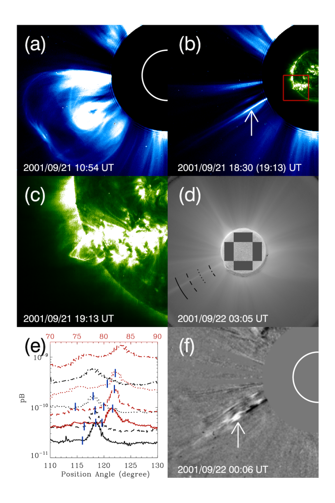
Figure 1.: (a) The white-light image observed by LASCO C2 at 10:54 UT for the event on 21 September 2001. (b) Composite image from LASCO C2 (18:30 UT) and EIT 195 Å (19:31 UT) showing the post-CME ray, as denoted by the white arrow, and the post-CME loops. (c) The enlarged version of the EIT image inside the red square in Figure 1(b). (d) pB data recorded by LASCO at 03:05 UT on 22 September 2001. The four arcs are at 3, 4, 5, and 6 R_⊙, along which the pB intensities are plotted in the next panel. (e) pB intensities in units of median solar brightness versus position angles at 3 (dot-dashed), 4 (dotted), 5 (dashed), and 6 (solid) R_⊙ for the 2001/09/21 event (black lines) and the 2002/01/08 event (red lines). (f) Running difference image at 00:06 on 22 September 2001 showing the presence of a blob structure. [See the electronic edition for a color version of this figure.]

Figure 2.: (a) Height-time profiles of the three blobs measured in the event on 21 September 2001 and represented by plus signs, stars, and diamonds. The lines are given by the second-order polynomial fitting to all the h-t data points. (b) Radial variations of the blob velocities deduced from the h-t fittings. The corresponding positions for the blobs are marked with the same symbols as that used in Figure 2(a).

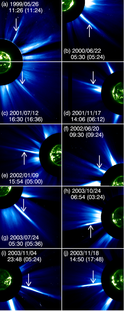
Figure 3.: Composite images from LASCO C2 and EIT 195 Å showing post-CME rays, denoted by the white arrows, and post-CME loops for the ten events. The observation time for LASCO is given in each panel, the time in parenthesis corresponds to the EIT data. [See the electronic edition for a color version of this figure.]

Figure 4.: Height-time profiles of blobs measured in the ten events shown in Figure 3. The blob occurrence order is indicated by various symbols.

Figure 5.: The fitted velocities of blobs as a function of heliocentric distance for the ten events shown in Figure 3. The blob occurrence order is indicated by the same symbols used in Figure 4.

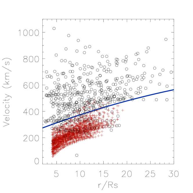
Figure 6.: Velocity-distance profiles for the 45 post-CME blobs collected in this study (black circles) and the 106 streamer-blobs (red pluses) given by Song et al. (2009). (The blue line is drawn to separate their velocity distributions.) The blue line, serving as a good separator of the two data sets, is given by the average of the polynomial fittings to the two groups of velocity measurements. [See the electronic edition for a color version of this figure.]

References

- Bemporad (2006) Bemporad, A., Poletto, G., Suess, S.T., Ko, Y.-K., Schwadron, N.A., Elliott, H.A., Raymond, J.C.:2006, Astrophys. J. 638, 1110
- Brueckner (1995) Brueckner, G.E., Howard, R.A., Koomen, M.J., Korendyke, C.M., Michels, D.J., Moses, J.D., et al.: 1995, Solar Phys. 162, 357.
- Carmichael (1964) Carmichael, H.: 1964, In: Hess, W. N. (ed.), The Physics of Solar Flares, NASA SP-50, 451.
- Chen (2011) Chen, Y., Feng, S.W., Li, B., Song, H.Q., Xia, L.D., Kong, X.L., Li, X.: 2011, Astrophys. J. 728, 147.
- Chen (2007) Chen, Y., Hu, Y.Q., Sun, S.J.: 2007, Astrophys. J. 665, 1421.
- Chen (2009) Chen, Y., Li, X., Song, H.Q., Shi, Q.Q., Feng, S.W., Xia, L.D.: 2009, Astrophys. J. 691, 1936.
- Chen (2010) Chen, Y., Song, H.Q., Li, B., Xia, L.D., Wu, Z., Fu, H., Li, X.: 2010, Astrophys. J. 714, 644.
- Ciaravella (2008) Ciaravella, A., Raymond, J.C.: 2008, Astrophys. J. 686, 1372.
- Ciaravella (2002) Ciaravella, A., Raymond, J.C., Li, J. Reiser, P., Gardner, L.D., Ko, Y.-K., Fineschi, S.: 2002, Astrophys. J. 575, 1116.
- Feng (2011) Feng, S.W., Chen, Y., Li, B., Song H.Q., Kong, X.L., Xia, L.D., Feng, X.S.: 2011, Solar Phys., 272, 119.
- Hirayama (1974) Hirayama, T.:1974, Solar Phys. 34, 323.
- Kaiser (2008) Kaiser, M. L., Kucera, T. A., Davila, J. M., Cyr, O. C. St., Guhathakurta, M., Christian, E.: 2008, Space Sci. Rev. 136, 5.
- Ko (2003) Ko, Y.-K., Raymond, J.C., Lin, J., Lawrence, G., Li, J., Fludra, A.: 2003, Astrophys. J. 594, 1068.
- Kohl (1995) Kohl, J.L., Esser, R., Gardner, L.D., Habbal, S., Daigneau, P.S., Dennis, E.F., et al.: 1995, Solar Phys. 162, 313.
- Kopp (1976) Kopp, R.A., Pneuman, G.W.:1976, Solar Phys. 50, 85.
- Lapenta (2005) Lapenta, G., Knoll, D.A.: 2005, Astrophys. J. 624, 1049.
- Lee (1988) Lee, L. C., Wang, S., Wei, C. Q.: 1988, J. Geophys. Res. 93, 7354.
- Lin (2000) Lin, J., Forbes, T.G.: 2000, J. Geophys. Res. 105, 2375.
- Lin (2005) Lin, J., Ko, Y.-K., Raymodn, J.C., Stenborg, G.A., Jiang, Y., Zhao, S., Mancuso, S.: 2005, Astrophys. J. 622, 1251.
- Lin (2009) Lin, J., Li, J., Ko, Y.-K., Raymond, J.C.: 2009, Astrophys. J. 693, 1666.
- Litvinenko (1996) Litvinenko, Y.: 1996, Astrophys. J. 462, 997.
- Liu (2009) Liu, Y., Luhmann, J.G., Lin, R.P., Bale, S.D.: 2009, Astrophys. J. Lett. 698 51.
- Patsourakos (2011) Patsourakos, S., Vourlidas, A.: 2011, Astron. Astrophys. 525, A27.
- Sheeley (1997) Sheeley, N. R., Wang, Y. M., Hawley, S. H., Brueckner, G. E., Dere, K. P., Howard, R. A., et al.: 1997, Astrophys. J. 484, 472.
- Song (2009) Song, H.Q., Chen, Y., Liu, K., Feng, S.W., Xia, L.D.: 2009, Solar Phys. 258, 129.
- Sturrock (1966) Sturrock, P.A.: 1966, Nature 211, 695.
- Vršnak (2009) Vršnak, B., Poletto, G., Vujić, E., Vourlidas, A., Ko, Y.-K., Raymond, J.C., et al.: 2009, Astron. Astrophys. 499, 905.
- Wang (1988) Wang, S., Lee, L. C., Wei, C. Q.: 1988, Phys. Fluids 31, 1544.
- Wang (2000) Wang, Y. M., Sheeley, N. R., Socker, D. J., Howard, R. A., Rich, N. B.: 2000, J. Geophys. Res. 105, 25133.
- Wang (1998) Wang, Y. M., Sheeley, N. R., Walters, J. H., Brueckner, G. E., Howard, R. A., Michels, D. J., et al.: 1998, Astrophys. J. Lett. 498, 165.
- Web (2003) Webb, D.F., Burkepile, J., Forbes, T.G., Riley, P.: 2003, J. Geophys. Res. 108, 1440.
- Winterhalter (1994) Winterhalter, D., Smith, E.J., Burton, M.E., Murphy, N., McComas, D.J.: 1994, J. Geophys. Res. 99, 6667.
- Wood (2005) Wood, P., Neukirch, T.: 2005, Solar Phys. 226, 73.