$\sin{\theta}_{13}$ and neutrino mass matrix with an approximate flavor symmetry

Abstract

For a neutrino mass matrix whose texture has an approximate flavor symmetry and where one has near degenerate neutrino mass, it is shown that the tribimaximal values for atmospheric angle $\sin^{2}{\theta_{23}}=\frac{1}{2}$ and solar angle $\sin^{2}{\theta_{12}}=\frac{1}{3}$ can be maintained even when the reactor angle $\theta_{13}\neq 0$. The non zero $\sin\theta_{13}$ implies approximate $\nu_{\mu}\rightarrow-\nu_{\tau}$ symmetry instead of $\nu_{\mu}\rightarrow\nu_{\tau}$ symmetry.

1 Introduction

There is compelling evidence that neutrinos change flavor, have non zero masses and that neutrino mass eigenstates are different from weak eigenstates. As such they undergo oscillations. The flavor and mass eigenstates are related by the so called Pontecorvo-Maki-Nakagawa-Sakata (PMNS) mixing matrix 1 ,

$$\left(\begin{tabular}[]{c}$\nu_{e}$\\ $\nu_{\mu}$\\ $\nu_{\tau}$\end{tabular}\right)=U\left(\begin{tabular}[]{c}$\nu_{1}$\\ $\nu_{2}$\\ $\nu_{3}$\end{tabular}\right),$$ (7)

where the matrix $U$ has been parameterized by the Particle Data Group (PDG) as 2

$$\left(\begin{tabular}[]{ccc}$c_{12}c_{13}$&$s_{12}c_{13}$&$s_{13}e^{-i\delta}$\\ $-s_{12}c_{23}-c_{12}s_{23}s_{13}e^{i\delta}$&$c_{12}c_{23}-s_{12}s_{23}s_{13}e^{i\delta}$&$s_{23}c_{13}$\\ $s_{12}s_{23}-c_{12}c_{23}s_{13}e^{i\delta}$&$-c_{12}s_{23}-s_{12}c_{23}s_{13}e^{i\delta}$&$c_{23}c_{13}$\end{tabular}\right)P=U_{PMNS}P.$$ (8)

Here $c_{ij}=\cos{\theta_{ij}}$, $s_{ij}=\sin{\theta_{ij}}$ and $P$ is a diagonal matrix which contains (Majorana) CP violating phases in addition to the (Dirac) CP violating phase $\delta$. $\theta_{12}$, $\theta_{23}$ and $\theta_{13}$ are respectively known as solar, atmospheric and reactor angles.

Current global fits allow the following ranges for the mass squared differences and mixing angles 2 :

$$7.05\times 10^{-5}eV^{2} \leq\Delta m_{12}^{2}\leq 8.34\times 10^{-5}eV^{2},$$

$$0.25 \leq\sin^{2}{\theta_{12}}\leq 0.37,$$

$$2.70\times 10^{-3}eV^{2} \leq\Delta m_{31}^{2}\leq 2.75\times 10^{-3}eV^{2},$$

$$0.36 \leq\sin^{2}{\theta_{23}}\leq 0.67,$$ (9)

with the following best fit (BF) values

$$\Delta m_{12}^{2}=7.65\times 10^{-5}eV^{2},\ \ \ \sin^{2}{\theta_{12}}=0.304,\ \ \ \Delta m_{31}^{2}=2.40\times 10^{-3}eV^{2},\ \ \ \sin^{2}{\theta_{23}}=0.5.$$ (10)

Recent results from T2K collaboration 3 and MINOS indicate a relatively large $\theta_{13}$ and when combined with the global fit gives 4

$$\sin^{2}{\theta_{13}}=0.025\pm 0.007.$$ (11)

There is further evidence for nonzero reactor also $\theta_{13}$ from DAYA BAY5 and RENO6 collaborations which respectively give

$$\theta_{13}=\left(8.83^{+0.81}_{-0.88}\right)^{o}\qquad\theta_{13}=\left(9.36^{+0.88}_{-0.96}\right)^{o}$$

It is interesting on its own right to consider non-zero value for $\sin^{2}{\theta_{13}}$ in the above range. In fact it has been shown by the author7 that nonzero value of $\sin^{2}{\theta_{13}}$ has important implications for the leptogenesis asymmetry parameter; its contribution to this parameter may even dominate.

Before we proceed further it is instructive to summarize the theoretical framework needed. The effective Majorana neutrino mass matrix $M_{\nu}$ constructed directly or in seesaw mechanism, can be symbolically written as 8

$$L=-\bar{L_{\ell}}M_{\ell}e_{R}-\bar{L_{\ell}}M_{D}N_{R}-N_{R}^{T}M_{R}N_{R}$$ (12)

where $L_{\ell}=(e_{L},v_{L})$ are lepton doublets, $e_{R}$ charged lepton $SU_{L}(2)$ singlets with non-vanishing hypercharge, $N_{R}$ are $SU_{L}(2)\times U(1)$ singlets. It is convenient to have a basis in which $M_{\ell}$ and $M_{R}$ are simultaneously diagonal

$$M_{\ell}\rightarrow\hat{M_{\ell}}=U_{L}^{{\dagger}}M_{\ell}U_{R},\,\,\,\,M_{R}\rightarrow\hat{M_{R}}=V^{T}M_{R}V$$ (13)

Correspondingly $L_{\ell}\rightarrow U_{L}L_{\ell},e_{R}\rightarrow U_{R}e_{R}$.

We can select a basis in which $U_{L}$ is diagonal i.e. $M_{\ell}$=diag$(m_{e},m_{\mu},m_{\tau})$. One may remark that the so called $2-3(\mu-\tau)$ symmetry can not be simultaneously valid for left-handed charged leptons and left-handed neutrinos. In the above basis it is obvious since $m_{\mu}\neq m_{\tau}$ but in fact it is independent of what basis one chooses 9 . Thus $2-3(\mu-\tau)$ symmetry can only be regarded as an effective (approximate) symmetry in the neutrino sector and was inspired by maximal atmospheric angle and $\theta_{r}=0$. If $\theta_{r}\neq 0$, it has to be violated.

Since the oscillation data are only sensitive to mass squared differences, they allow for three possible arrangements of different mass levels 8 . It is customary to order the mass eigenstates such that $m_{1}^{2}<m_{2}^{2}$. We have two squared mass differences:

$\Delta m^{2}_{21}=m^{2}_{2}-m^{2}_{1}=\delta m^{2}$, $\Delta m^{2}=m_{3}^{2}-\frac{m^{2}_{2}+m^{2}_{1}}{2}$, where $\Delta m^{2}>0$ for normal hierarchy ($m_{1}$ $\lesssim m_{2}$ $\leq m_{3}$) and $<0$ for inverted hierarchy $(m_{1}\simeq m_{2}\gg m_{3})$. For degenerate case $(m_{1}\simeq m_{2}\simeq m_{3})$, one can write neutrino mass matrix as

$$M_{\nu}=m_{0}I+\delta M_{\nu}$$ (14)

where $\delta M_{\nu}\ll m_{0}$ or

$$M_{\nu}=m_{o}\left(\begin{array}[]{ccc}1&0&0\\ 0&0&1\\ 0&1&0\\ \end{array}\right)+\delta M_{\nu}$$ (15)

in case of opposite CP-parity of $\nu_{2}$ and $\nu_{3}$ ($m_{2}$ and $m_{3}$ are of opposite sign).

We have three mixing angles $\theta_{12}=\theta_{s}$ (solar), $\theta_{23}=\theta_{a}$ (atmospheric) and $\theta_{13}=\theta_{r}$ (reactor). Some new ingredients are needed to describe correctly the three mixing angles. However it is well known that the best fit values given in Eq. (10) are consistent with the so called tribimaximal (TB) mixing 10 corresponding to

$$\sin^{2}{\theta_{12}}=\frac{1}{3},\ \ \ \sin^{2}{\theta_{23}}=\frac{1}{2},\ \ \ \sin^{2}\theta_{13}=0.$$ (16)

For our discussion it is convenient to state various symmetries and/or conditions on $M_{\nu}$ which lead to $\theta_{13}=0$ and TB mixing. In an obvious notation if one has 2-3 symmetry i.e. $(M_{\nu})_{22}=(M_{\nu})_{33}$ and $(M_{\nu})_{12}=(M_{\nu})_{13}$, then $\theta_{13}=0$ and $\sin^{2}\theta_{23}=1/2$. If further $(M_{\nu})_{11}+(M_{\nu})_{12}=(M_{\nu})_{22}+(M_{\nu})_{23}$, then we have TB mixing given in Eq. (1.12).

Recently, a possibility has been discussed 11 (named TBR) which allows the extension of TB mixing, so as to have a non-zero value of $\theta_{13}$, preserving at the same time the predictions for the TB solar angle [$\sin^{2}{\theta_{12}}=\frac{1}{3}$] and the maximal atmospheric angle [$\sin^{2}{\theta_{23}}=\frac{1}{2}$].

To implement TBR, it is generally assumed that

$$M_{\nu}^{TBR}=M_{\nu}^{TB}+\delta M_{\nu}$$ (17)

$M_{\nu}^{TB}$ satisfies the conditions mentioned above. The various recent attempts in this aspect differ in the treatment of $\delta M_{\nu}$. In general $\delta M_{\nu}$ contains six parameters. In 12 , the conditions on these parameters are put so as to give $\theta_{r}\neq 0$ but $|\theta_{23}-45|\ll 1$, fixing $\theta_{s}$ at the TB value. However these conditions are not unique. A simple form for $\delta M_{\nu}$ for normal hierarchy is also invented12 . In 13 ; 14 , $\delta M_{\nu}$ is realized in specific flavor symmetry models based on $S_{4}$ and $A_{4}$ symmetries respectively.

In this paper we attempt to realize TBR in degenerate mass spectrum given in Eq. (14) which as we shall see has some attractive features.

2 Approximate flavor symmetry and diagonalization of neutrino mass matrix

For degenerate case a particularly attractive Majorana neutrino mass matrix, which is a multiple of unit matrix supplemented by three far smaller off-diagonal entries, is given by 15 ; 16

$$M_{\nu}=m_{0}\left(\begin{tabular}[]{ccc}$1$&$\epsilon_{12}$&$\epsilon_{13}$\\ $\epsilon_{12}$&$1$&$\epsilon_{23}$\\ $\epsilon_{13}$&$\epsilon_{23}$&$1$\end{tabular}\right)=m_{0}I+\delta M_{\nu},$$ (18)

with $\epsilon_{ij}\ll 1$. This implies that in the limit of off-diagonals going to zero, $M_{\nu}$ is flavor blind or preserves flavor symmetry. When they are switched on, but being at least an order of magnitude smaller than diagonal elements, they violate it as small perturbations

A particularly attractive realization of $\delta\mathit{M_{\nu}}$ given in Eq. (18)is provided by Zee model 17 where diagonal elements are vanishing and off-diagonal elements arise from radiative corrections18 .

Another realization of $\delta M_{\nu}$ in Eq.(18) is provided by a simple extension of the standard electroweak group to 16

$$G\equiv SU_{L}(2)\times U_{\ell}(1)\times U_{\mu}(1)\times U_{\tau}(1)$$

In addition to usual fermions there are three right-handed $SU_{L}(2)$ singlet neutrinos which carry appropriate $U_{i}(1)$ quantum numbers. Further in addition to $SU_{L}(2)$ Higgs doublets, there are three Higgs $SU_{L}(2)$ singlets $\Sigma^{i}$ with appropriate $U_{i}(1)$ quantum numbers. The fermions and Higgs bosons are assigned to the following representations of the group $G$:

$$L^{(1)}=L_{e}=\left[\begin{array}[]{c}\nu_{e}\\ e\end{array}\right]_{L}:(2,-1,0,0):\phi^{(1)}$$

$$e_{R}:(1,-2,0,0),\qquad N_{e}:(1,-1,1,0);\qquad\Sigma^{(1)}:(1,1,-1,0)$$

$$L^{(2)}=L_{\mu}=\left[\begin{array}[]{c}\nu_{\mu}\\ \mu\end{array}\right]_{L}:(2,0,-1,0):\phi^{(2)}$$

$$\mu_{R}:(1,0,-2,0),\qquad N_{\mu}:(1,1,0,-1);\qquad\Sigma^{(2)}:(1,-1,0,1)$$

$$L^{(3)}=L_{\tau}=\left[\begin{array}[]{c}\mu_{\tau}\\ \tau\end{array}\right]_{L}:(2,0,0,-1):\phi^{(3)}$$

$$\tau_{R}:(1,0,0,-2),\qquad N_{\tau}:(1,0,-1,1);\qquad\Sigma^{(3)}:(1,0,1,-1)$$ (19)

The Yukawa couplings of neutrinos with Higgs are given by

$$L_{Y}= \sum_{i=e,\mu,\tau}g_{i}(\bar{L}^{(i)}\tilde{\phi}^{(i)}e_{R}^{(i)}+\text{H.C.})$$

$$+\sum_{i=d,s,b}G_{i}(\bar{q}_{L}^{(i)}\tilde{\phi}^{(i)}q_{R}^{(i)}+\text{H.C.})$$

$$+\sum_{i=u,c,t}G_{i}(\bar{q}_{L}^{(i)}\phi^{(i)}q_{R}^{(i)}+\text{H.C.})$$

$$+(h_{11}\bar{L}_{e}N_{e}\phi^{(2)}+h_{23}\bar{L}_{\mu}N_{\tau}\phi^{(3)}+h_{32}\bar{L}_{\tau}N_{\mu}\phi^{(1)}+\text{H.C.})$$

$$+\left[f_{12}(N_{e}^{T}cN_{\mu}+N_{\mu}^{T}cN_{e})\tilde{\Sigma}^{(3)}\right.$$

$$\left.+f_{13}(N_{e}^{T}CN_{\tau}+N_{\tau}^{T}CN_{e})\tilde{\Sigma}^{(2)}\right.$$

$$\left.+f_{23}(N_{\mu}^{T}CN_{\tau}+N_{\tau}^{T}CN_{\mu})\tilde{\Sigma}^{(1)}+\text{H.C.}\right]$$ (20)

where

$$\phi=\left(\begin{tabular}[]{c}$\phi^{o}$\\ $-\phi$\end{tabular}\right),\qquad\tilde{\phi}=-i\tau_{2}\phi^{*}=\left(\begin{tabular}[]{c}$\phi^{\dagger}$\\ $\phi^{o}$\end{tabular}\right)$$

The symmetry is spontaneously broken by giving vacuum expectation values to Higgs bosons $\phi^{(i)},\Sigma^{(i)}$:

$$\langle\phi^{(i)}\rangle=\frac{v_{i}}{\sqrt{2}},\qquad\langle\Sigma^{(i)}\rangle=\frac{\Lambda_{i}}{\sqrt{2}}$$

where $\Lambda_{i}\gg v_{i}$ so that extra gauge bosons which break the $e-\mu-\tau$ universality become super heavy and so do the right handed neutrinos. For simplicity we shall take, $v_{1}=v_{2}=v_{3}$ and $\Lambda_{1}=\Lambda_{2}=\Lambda_{3}$ (any differences can be absorbed in the corresponding Yukawa coupling constants with the Higgs bosons). Then the charged lepton and Dirac neutrino mass matrices are

$$M_{\ell}=\frac{v}{\sqrt{2}}\left(\begin{tabular}[]{ccc}$g_{1}$&$0$&$0$\\ $0$&$g_{2}$&$0$\\ $0$&$0$&$g_{3}$\end{tabular}\right)$$ (21)

$$m_{D}=\frac{v}{\sqrt{2}}\left(\begin{tabular}[]{ccc}$h_{11}$&$0$&$0$\\ $0$&$0$&$h_{23}$\\ $0$&$h_{32}$&$0$\end{tabular}\right)$$ (22)

while $M_{R}$ is

$$M_{R}=\frac{1}{\sqrt{2}}\left(\begin{tabular}[]{ccc}$0$&$f_{12}\Lambda_{1}$&$f_{13}\Lambda_{1}$\\ $f_{12}\Lambda_{1}$&$0$&$f_{23}\Lambda_{1}$\\ $f_{13}\Lambda_{1}$&$f_{23}\Lambda_{1}$&$0$\end{tabular}\right)$$ (23)

Then the effective Majorana mass matrix for the light neutrinos is

$$\delta M_{\nu}=\hat{m}_{D}\hat{M}_{R}^{-1}\hat{m}_{D}^{T}$$ (24)

where $\hat{m}_{D}$ is the Dirac matrix in $(\bar{N}_{1}\quad\bar{N}_{2}\quad\bar{N}_{3})\left(\begin{tabular}[]{c}$\nu_{e}$\\ $\nu_{\mu}$\\ $\nu_{\tau}$\end{tabular}\right)$ basis giving

$$\delta M_{\nu}=\frac{v^{2}}{2M_{1}}\left(\begin{tabular}[]{ccc}$-h_{11}^{2}$&$h_{11}h_{23}$&$h_{11}h_{32}$\\ $h_{23}h_{11}$&$-h_{23}^{2}$&$h_{23}h_{32}$\\ $h_{32}h_{11}$&$h_{23}h_{32}$&$-h_{32}^{2}$\end{tabular}\right)$$ (28)

Here $M_{1}=f_{1}\displaystyle{\frac{1}{\sqrt{2}}}$ taking all Yukawa couplings in $M_{R}$ equal.

In order to generate $M_{\nu}^{0}$, we introduce a right handed neutrino $N$ and a corresponding Higgs boson $\Sigma$, both of which are $SU_{L}(2)$ and $[U(1)]^{3}$ singlets, with the Yukawa coupling

$$L_{Y}^{o}=(h_{1}\bar{L_{e}}\phi^{(1)}+h_{2}\bar{L_{\mu}}\phi^{(2)}+h_{3}\bar{L_{\tau}}\phi^{(3)})N+\text{H.C.}+fN^{T}CN\Sigma$$ (29)

Although a term $M_{N}N^{T}CN$ is allowed in (29) but it can be absorbed in $\displaystyle{\frac{f\Lambda}{\sqrt{2}}}$ after the symmetry breaking. After spontaneous symmetry breaking $\langle\Sigma\rangle=\displaystyle{\frac{\Lambda}{2}}$(so that $M=f\Lambda/\sqrt{2}$) and in the basis $\bar{N}\left(\begin{tabular}[]{c}$\nu_{e}$\\ $\nu_{\mu}$\\ $\nu_{\tau}$\end{tabular}\right)$, the Dirac neutrino mass matrix, $m_{D}^{o}$ is $3\times 1$ matrix

$$m_{D}^{o}=\left(\begin{tabular}[]{c}$h_{1}$\\ $h_{2}$\\ $h_{3}$\\ \end{tabular}\right)\frac{v}{\sqrt{2}}$$ (30)

The effective neutrino mass matrix is then

$$M_{\nu}^{o}=m_{D}^{o}(m_{D}^{o})^{T}\frac{1}{M}=\frac{v^{2}}{2M}\left(\begin{tabular}[]{ccc}$h_{1}^{2}$&$0$&$0$\\ $0$&$h_{2}^{2}$&$0$\\ $0$&$0$&$h_{3}^{2}$\end{tabular}\right)$$ (31)

Now $\Sigma^{i}$ carry flavor quantum numbers of $U_{i}$ but $\Sigma$ does not, being $[U(1)]^{3}$ singlet, and we may take $\langle\Sigma^{i}\rangle\gg\langle\Sigma\rangle$ so that $M_{1}\gg M$ and then, as in clear from Eqs.(28) and (31), $\delta M_{\nu}\ll M_{\nu}^{0}$. This also justifies neglect of mixing of $N$ with $N^{(i)}$. In a way it is nice since in fermions mass hierarchy, Yukawa couplings widely differ. Here it is due to $M_{1}\gg M$ while Yukawa couplings are of same order. With $h_{1}\simeq h_{2}\simeq h_{3}$, we have the required matrix given in Eq.(18) or its variant to be considered later, [c.f. Eq.(40)]. We may remark here that although the Lagrangian (29) as it stands is not flavour blind, but if one takes $h_{1}=h_{2}=h_{3}=h$, then it is flavor singlet. This is easy to see as follows. In three dimensional flavor space, introduce two vectors $\textbf{L}=(L_{1},L_{2},L_{3})$ and $\boldsymbol{\Phi}=(\phi_{1},\phi_{2},\phi_{3})$, then the Lagrangian (29) takes the form

$$L^{0}_{Y}=h[\bar{\textbf{L}}.\boldsymbol{\Phi}N+\text{H.C.}]+fN^{T}CN\Sigma$$

which is flavor single, just as $(\boldsymbol{\bar{\Sigma}}.\boldsymbol{\pi})\Lambda$ is singlet under isospin in hadron physics. When the symmetry is broken, $M_{\nu}^{0}$ is then a multiple of unit matrix (flavor blind) and since it dominates over $\delta M_{\nu}$, $M_{\nu}$ has approximate flavor symmetry. It is in this limited sense that we talk about approximate falvor symmetry.

We now explore the TBR possibility for the diagonalization of the neutrino mass matrix given in Eq. (18). In spite of its attractiveness, its diagonalization is in conflict with the neutrino data. It is instructive to show it as it would provide us a guidance for possible modification of $M_{\nu}$ in Eq. (18) to obtain agreement with the experimental data. The diagonalization of $M_{\nu}$ (we need to consider the diagonalization of $\delta M_{\nu}$ as $m_{0}I$ commutes with any diagonalyzing matrix) give among others the following relation 9

$$\epsilon_{2}=\frac{\cos^{2}\theta_{s}-\tan^{2}\theta_{r}}{\sin^{2}\theta_{s}-\tan^{2}\theta_{r}}\epsilon_{1},\quad\epsilon_{1}+\epsilon_{2}+\epsilon_{3}=0$$ (32)

where $\epsilon_{i}$ are the eigenvalues of $\delta M_{\nu}$.

Now

$$m_{2}=m_{0}(1+\epsilon_{2}),\text{ }m_{1}=m_{0}(1+\epsilon_{1}),\text{ }m_{3}=m_{0}(1-\epsilon_{1}-\epsilon_{2})$$ (33)

The first of relations (33) give

$$\epsilon_{+}(1-2\tan^{2}\theta_{r})=\epsilon_{-}\cos 2\theta_{s}$$ (34)

while

$$\Delta m^{2}_{12}=4m^{2}_{0}\epsilon_{-}$$ (35a)

$$\Delta m^{2}=-6m^{2}_{0}\epsilon_{+}$$ (35b)

where

$$\epsilon_{+}=\frac{\epsilon_{2}+\epsilon_{1}}{2},\text{ }\epsilon_{-}=\frac{\epsilon_{2}-\epsilon_{1}}{2}$$ (36)

We require $\epsilon_{-}\ll\epsilon_{+}$ and the relation (34) then implies that $tan^{2}\theta_{r}\simeq 1/2$, contrary to the experimental data. The relation (32) is the consequence of det$|\delta M_{\nu}|=0$. To avoid this, the simplest extension is that

$$\delta M_{\nu}=m_{o}\left(\begin{array}[]{ccc}a&\epsilon_{12}&\epsilon_{13}\\ \epsilon_{12}&0&\epsilon_{23}\\ \epsilon_{13}&\epsilon_{23}&0\end{array}\right)$$ (40)

where $a\ll 1$. Then the relations in Eq. (32) are replaced by

$$a=-\epsilon_{1}(\tan^{2}\theta_{r}-cos^{2}\theta_{s})-\epsilon_{2}(\tan^{2}\theta_{r}-\sin^{2}\theta_{s})$$

$$=\epsilon_{+}(1-2\tan^{2}\theta_{r})-\epsilon_{-}\cos 2\theta_{s}$$ (41)

$$\epsilon_{1}+\epsilon_{2}+\epsilon_{3}=a$$ (42)

Further while the relation (35a) remains the same but (35b) is changed to

$$\ \Delta m^{2} = m_{0}^{2}[2a-6\epsilon_{+}]$$ (43a)

$$= -4m_{0}^{2}[\epsilon_{+}(1+\frac{1}{2}\tan^{2}\theta_{r})+\frac{1}{2}\epsilon_{-}\cos 2\theta_{s})]$$

On using Eq. (35a)

$$|\Delta m^{2}|=4m_{0}^{2}\epsilon_{+}(1+\tan^{2}\theta_{r})+\frac{1}{2}\cos\theta_{s}\Delta m_{12}^{2}$$

Since $$|\Delta m^{2}|\gg\Delta m_{12}^{2}$$, it follows that

$$|\Delta m^{2}|\simeq 4m_{0}^{2}|\epsilon_{+}|$$ (43b)

Thus from Eqs. (35a), (43b) and (10)

$$\left|\frac{\epsilon_{-}}{\epsilon_{+}}\right|=\frac{\Delta m_{12}^{2}}{|\Delta m^{2}|}=3.2\times 10^{-2}$$ (44)

The other relations which diagonalization give are

$$\cos 2\theta_{a}\epsilon_{+}-\sin 2\theta_{a}\sin 2\theta_{s}\sin\theta_{r}\epsilon_{-}=0$$ (45)

$$\epsilon_{12}+\epsilon_{13}=\cos\theta_{r}\sin 2\theta_{s}(\cos\theta_{a}-\sin\theta_{a})\epsilon_{-}-2(\cos\theta_{a}+\sin\theta_{a})\tan\theta_{r}\epsilon_{+}$$ (46)

$$\epsilon_{12}-\epsilon_{13}=\cos\theta_{r}\sin 2\theta_{s}(\cos\theta_{a}+\sin\theta_{a})\epsilon_{-}+2(\cos\theta_{a}-\sin\theta_{a})\tan\theta_{r}\epsilon_{+}$$ (47)

$$\epsilon_{23}=-\sin 2\theta_{a}(\epsilon_{+}+\epsilon_{-}\cos 2\theta_{s})-\epsilon_{-}\cos 2\theta_{a}\sin 2\theta_{s}\sin\theta_{r}$$ (48)

To proceed further it is convenient to use the expansion about the maximum atmospheric angle $\sin^{2}\theta_{a}=\frac{1}{2}$

$$\sin\theta_{a}=-\frac{1}{\sqrt{2}}(1+t),\text{ }\cos\theta_{a}=\frac{1}{\sqrt{2}}(1-t),\text{ }\sin^{2}\theta_{a}=0.5+t$$ (49)

Then the relations (45-48) simplify to

$$-2t\epsilon_{+}+\sin 2\theta_{s}\sin\theta_{r}\epsilon_{-} = 0$$ (50)

$$\epsilon_{12}-\epsilon_{13} = -\sqrt{2}t\cos\theta_{r}\sin 2\theta_{s}\epsilon_{-}+2\sqrt{2}\tan\theta_{r}\epsilon_{+}$$ (51)

$$\epsilon_{23} = \epsilon_{+}+\epsilon_{-}\cos 2\theta_{s}$$ (52)

$$\epsilon_{12}+\epsilon_{13} = \sqrt{2}\cos\theta_{r}\sin 2\theta_{s}\epsilon_{-}+2\sqrt{2}t\tan\theta_{r}\epsilon_{+}$$ (53)

$$= \sqrt{2}\sin 2\theta_{s}(1-\frac{3}{2}\sin^{2}\theta_{r})\epsilon_{-}$$

where in the second step we have used Eq. (50). Further from Eqs. (41) and (52)

$$a-\epsilon_{23}=-2\epsilon_{+}\tan^{2}\theta_{r}-2\epsilon_{-}\cos 2\theta_{s}$$ (54)

so that together with Eq. (53)

$$\tan 2\theta_{s}=\frac{-\sqrt{2}(\epsilon_{12}+\epsilon_{13})(1+\frac{3}{2}\sin^{2}\theta_{r})}{a-\epsilon_{23}+2\tan^{2}\theta_{r}\epsilon_{+}}$$ (55)

We note that if $\nu_{\mu}\leftrightarrow\nu_{\tau}(2\leftrightarrow 3)$ symmetry is imposed so that $\epsilon_{12}=\epsilon_{13}$, $t\rightarrow 0$, $\theta_{r}\rightarrow 0$, the relations (50), (51) are identically satisfied. Further if $a-\epsilon_{23}=-\epsilon_{12}$, then Eq. (55) gives $\tan 2\theta_{s}=2\sqrt{2}$ i.e. the TB solar angle.

However if $\sin\theta_{r}\neq 0$, Eq. (50) implies that

$$\sin\theta_{r}=\frac{2t}{\sin 2\theta_{s}}\frac{\epsilon_{+}}{\epsilon_{-}}$$

$$\simeq\pm\frac{1}{\sqrt{2}}t\times 10^{2},$$ (56)

on using Eq. (44) and the TB value of $\theta_{s}$. This can accommodate any finite value of $\sin\theta_{r}$ for extremely small deviation from the maximal atmospheric angle $\sin^{2}\theta_{a}=\frac{1}{2}$.

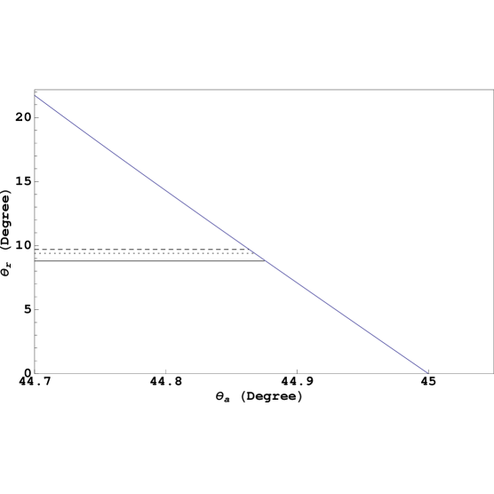
Figure 1: $\theta_{r}$ as a function of $\theta_{a}$. The solid, dotted and dashed lines respectively correspond to the best fit values for DAYA BAY, RENO and T2K collaborations.

Putting $t$ as given in the third relation of Eq.(49) in Eq.(56), we plot $\theta_{r}$ as a function of $\theta_{a}$ in Fig.1 which is if sign is taken negative in Eq.(56). If the sign is positive, $\theta_{a}$ is greater than $45^{\circ}$ and for $\theta_{r}=10^{\circ}$ it is $45.1^{\circ}$. It is clear that one can achieve $\theta_{r}\simeq 7^{\circ}$ to $10^{\circ}$, keeping $\theta_{a}$ around $45^{\circ}$. Thus it covers recently measured values of $\theta_{r}$ by $T2K$, DAYA BAY5 and RENO collaboration6 . It follows from Eq. (55) that TB solar angle is obtained i.e. $\tan 2\theta_{s}=2\sqrt{2}$, if

$$a-\epsilon_{23}+2\tan^{2}\theta_{r}\epsilon_{+}=-\frac{1}{2}(\epsilon_{12}+\epsilon_{13})(1+\frac{3}{2}\sin^{2}\theta_{r})$$ (57)

It remains to determine the parameters in the $\delta M_{\nu}$ given in Eq. (40). It follows from Eqs. (43b), (52), (53) and (54) that

$$|\epsilon_{23}|\simeq a\simeq|\epsilon_{+}|=\frac{1}{4}\frac{|\Delta m^{2}|}{m_{0}^{2}}$$ (58)

$$\frac{\epsilon_{12}+\epsilon_{13}}{\epsilon_{+}}\simeq\sqrt{2}\sin 2\theta_{s}\frac{\epsilon_{-}}{\epsilon_{+}}\simeq 4\times 10^{-2}$$ (59)

On the other hand from Eqs. (11) and (51)

$$\left|\frac{\epsilon_{12}-\epsilon_{13}}{\epsilon_{+}}\right|\simeq 2\sqrt{2}\tan\theta_{r}\simeq 4\times 10^{-1}$$ (60)

Thus it is possible to have TB solar angle $\sin^{2}\theta_{s}=\frac{1}{3}$ and almost maximal atmospheric angle $\sin^{2}\theta_{a}\simeq\frac{1}{2}$ and non zero $\sin^{2}\theta_{r}$ but at the cost of $\nu_{\mu}\rightarrow\nu_{\tau}$ symmetry as the relations (59) and (60) would imply. Finally the oscillation data give only a lower bound on the heaviest of the neutrino mass $m_{h}\geq|\Delta m^{2}|>0.05$eV but cannot fix it. However $m_{0}$ is further constrained by WMAP data, $\sum m_{i}<(0.4-0.7)$eV. Taking $m_{0}\simeq 0.1$eV, we get from Eqs. (10), (58), (59) and (60) that

$$|\epsilon_{23}|\simeq a\simeq|\epsilon_{+}|\simeq 6\times 10^{-2}$$

$$\epsilon_{12}+\epsilon_{13}\simeq 2.4\times 10^{-3}$$

$$|\epsilon_{12}-\epsilon_{13}|\simeq 2.4\times 10^{-2}$$

Then

$$\epsilon_{12}\simeq-\epsilon_{13}\simeq 10^{-2}$$ (61)

if the sign is chosen to be positive for $\frac{\epsilon_{-}}{\epsilon_{+}}$. If the sign is negative, $\epsilon_{12}$ and $\epsilon_{13}$ should be interchanged. This is meant for the rest of the manuscript.

We may remark here that there are four parameters, apart from $m_{o}$, in Eq.(40). There are two mass differences and three mixing angles. Thus the prediction one gets is a relationship between $\theta_{r}$ and $\theta_{a}$ which is shown in Fig.1. All above parameters as well Fig.1 are obtained by using best fit values given in Eq.(10).

All the values given in Eq.(61)are consistent with small perturbations (at least an order of magnitude smaller) to $M_{\nu}=m_{0}I$, $I$ being the unit matrix. It is important to note that Eq. (61) implies approximate $\nu_{\mu}\rightarrow-\nu_{\tau}$ symmetry (instead of $\nu_{\mu}\rightarrow\nu_{\tau}$ symmetry,which would imply $\epsilon_{12}-\epsilon_{13}=0$). On the other hand the exact $\nu_{\mu}\rightarrow-\nu_{\tau}$ symmetry would imply $\epsilon_{12}=-\epsilon_{13}$ i.e. $\epsilon_{12}+\epsilon_{13}=0$. In order to see how this happens for $\theta_{r}\neq 0$, we note from Eqs. (44), (59) and (60) that

$$\frac{\epsilon_{13}}{\epsilon_{12}}=\frac{1-\frac{1}{\sqrt{2}}10^{2}\tan(\theta_{r})}{1+\frac{1}{\sqrt{2}}10^{2}\tan(\theta_{r})}$$ (62)

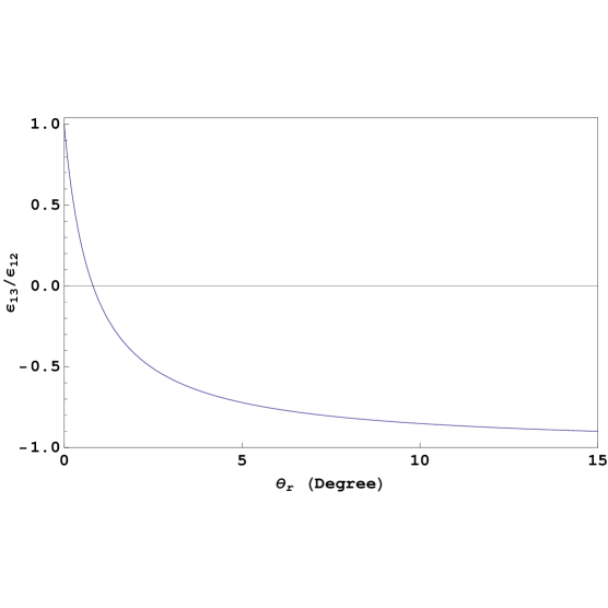
Figure 2: $\displaystyle{\epsilon_{13}/\epsilon_{12}}$ as a function of $\theta_{r}$.

In Fig. 2, we plot $\epsilon_{13}/\epsilon_{12}$ as a function of $\theta_{r}$. We see how the transition from exact $\nu_{\mu}\rightarrow\nu_{\tau}$ symmetry $(\epsilon_{12}/\epsilon_{13}=1)$ at $\theta_{r}=0$ to approximate $\nu_{\mu}\rightarrow-\nu_{\tau}$ symmetry $\left(\displaystyle{\frac{\epsilon_{13}}{\epsilon_{12}}}\simeq-1,\text{e.g. at }\theta_{r}\simeq 10^{\circ},\displaystyle{\frac{\epsilon_{13}}{\epsilon_{12}}}\approx-0.85\right)$ takes place.

3 Summary and Conclusion

We have considered a model of approximate flavor symmetry which has near degenerate neutrino mass. It is shown that it is possible to have nonzero reactor angle while preserving the TB solar angle $\sin^{2}\theta_{s}=\frac{1}{3}$ and near maximal atmospheric angle $\sin^{2}\theta_{a}\simeq 0.5$.The non-zero $\sin\theta_{r}$ implies approximate $\nu_{\mu}\rightarrow-\nu_{\tau}$ symmetry rather than that $\nu_{\mu}\rightarrow\nu_{\tau}$ symmetry.

References

(1) B. Pontecorvo, Sov. Phys. JETP 6 (1957) 429 [Zh. Eksp.
Teor. Fiz. 33 (1957) 549]; Z. Maki, M. Nakagawa and S. Sakata, Prog.
theor. Phys. 28 (1962) 870.
(2) K. Nakamura et al. (Particle Data Group), J. Phys. G 37 (2010) 075021.
(3) T. Schwertz, M. Tortala, and J. W. F Valle, [arXiv: 1108.1376]; G. L. Fogli, E. Lisi, A. Marrone, A. Palazzo and A. M. Rotunno, [arXiv:1106.6028].
(4) K. Abe et al. (T2K collaboration), arXiv:1106.2822.
(5) F. P. An et al. (Daya Bay Collobation), arXiv: 1203.1669[hep-ex].
(6) J.K. Ahn et al (RENO colleboration): arXiv: 1204.0626[hep-ex].
(7) Riazuddin, Phys. Rev. D 81 (2010) 057301.
(8) For a review see, for example, R. N.Mohapatra and A.Y. Smirnov: arXiv:0603118, Ann Rev. Nucl. Part. Sci 59 (2006) 569 .
(9) C.S. Lam, Phys. Lett. B 507 (2001) 214 ; Phys. Rev. D 71 (2003) 093001
(10) P.F. Harrison, D. H. Perkins and W. G. Scott, Phys. Lett. B 530 (2002) 167
(11) S. F. King, arXiv:0903.3199v5.
(12) T. Araki, Phys. Rev. D 84 (2011) 037301 , arXiv: 1106.5211
(13) S. Morisi, K. M. Patel and E. Peinado, Phys. Rev. D 84 (2011) 053002, arXiv: 1107.0696.
(14) S. F. King and C. Luhn, arXiv: 1112.1959.
(15) S. L. Glashow, arXiv: 0912.4976.
(16) Fayyazuddin and Riazuddin, Phys. Rev. D 35 (1987) 2201; Riazuddin, JHEP 10 (2003) 009; Riazuddin, Phys. Rev. D 63 (2001) 033003.
(17) A. Zee, Phys. Lett. B 93 (1980) 389. For a recent discussion of this model, see ref. [16].
(18) Xiao-Gang He and S.K.Majee, arXiv: 1111.2293v.2
(19) J.Matsuda, C.J.Jarlskog, S.Skadhauf and M.Tanimoto, hep-ph0005147; Riazuddin, 3rd reference in [13].