Entanglement of polar symmetric top molecules as candidate qubits

Abstract

Proposals for quantum computing using rotational states of polar molecules as qubits have previously considered only diatomic molecules. For these the Stark effect is second-order, so a sizable external electric field is required to produce the requisite dipole moments in the laboratory frame. Here we consider use of polar symmetric top molecules. These offer advantages resulting from a first-order Stark effect, which renders the effective dipole moments nearly independent of the field strength. That permits use of much lower external field strengths for addressing sites. Moreover, for a particular choice of qubits, the electric dipole interactions become isomorphous with NMR systems for which many techniques enhancing logic gate operations have been developed. Also inviting is the wider chemical scope, since many symmetric top organic molecules provide options for auxiliary storage qubits in spin and hyperfine structure or in internal rotation states.

I Introduction

In principle, a quantum computer can perform a variety of calculations with exponentially fewer steps than a classical computer Bennett ; Deutsch ; Feynman ; Shor ; Grover ; Chuang . This prospect has fostered many proposals for means to implement a quantum computer Seth ; DiVincenzo ; Gershenfeld ; Cory ; Kane ; Loss ; Demille ; wallraff ; Lee ; andre ; yelin . Using arrays of trapped ultracold polar molecules is considered a promising approach, particularly since it appears feasible to scale up such systems to obtain large networks of coupled qubits Demille ; andre ; yelin ; carr ; Book2009 ; Friedrich ; Kotochigova ; Micheli ; Charron ; kuz ; ni ; lics ; YelinDeMille ; Wei1 ; Wei2 . Molecules offer a variety of long-lived internal states, often including spin or hyperfine structure as well as rotational states. The dipole moments available for polar molecules provide a ready means to address and manipulate qubits encoded in rotational states via interaction with external electric fields as well as photons.

Entanglement of qubit states, a major ingredient in quantum computation algorithms, occurs in polar molecule arrays by dipole-dipole interactions. In a previous study, we examined how the external electric field, integral to current designs for quantum computation with polar molecules, affects both the qubit states and the dipole-dipole interaction Wei2 . As in other work concerned with entanglement of electric dipoles, we considered diatomic or linear molecules, for which the Stark effect is ordinarily second-order. Consequently, a sizable external field ($\sim$several kV/cm) is required to obtain the requisite effective dipole moments in the laboratory frame.

In considering the operation of a key quantum logic gate (CNOT), we evaluated a crucial parameter, $\triangle\omega$, due to the dipole-dipole interaction. This is the shift in the frequency for transition between the target qubit states when the control qubit state is changed. For candidate diatomic molecules, under anticipated conditions for proposed designs, $\triangle\omega$ is very small ($\sim$20-60 kHz). It is essential to be able to resolve the $\triangle\omega$ shift unambiguously, but in view of line broadening expected with a sizeable external field, whether that will be feasible remains an open question Wei2 .

This question led us to consider polar symmetric top molecules, for which the Stark effect is first-order in most rotational states. The effective dipole moments are then nearly independent of the field strength. That enables use of a much lower external field (a few V/cm) to address and manipulate the dipoles, improving prospects for resolving the $\triangle\omega$ shift. The constancy of the symmetric top effective dipole moments also makes entanglement properties of electric dipole interactions isomorphous with those for nuclear magnetic resonance systems. This suggests that NMR techniques, extensively developed for quantum computation but limited in application by the small size of nuclear spins and scalability prospects Seth ; Cory2 ; Lieven might find congenial applications with qubit systems comprised of polar symmetric top molecules.

II EIGENSTATES FOR A POLAR SYMMETRIC TOP

The Hamiltonian for a single trapped polar symmetric top molecule in an external electric field may be written

$${\bf H}={\bf H}_{R}+{\bf H}_{S}+{\bf H}_{T}+{\bf H}_{s.q}$$ (1)

The major term is the rotational energy

$${\bf H}_{R}=B{\mathbf{J}}^{2}+(A-B){\mathbf{J}}_{z}^{2}$$ (2)

where $\mathbf{J}$ denotes the total rotational angular momentum and ${\mathbf{J}}_{z}$ its projection on the symmetry axis; A and B, the rotational constants, nominally inversely proportional to the moments of inertia about the principal axes along and perpendicular to the symmetry axis, respectively (actually effective values averaged over vibration and centrifugal distortion of the molecule). The Stark energy from interaction with the external electric field is

$${\bf H}_{S}=-\bm{\mu}\cdot\text{\Large\bm{$\varepsilonup$}}=-{\bf\mu}\text{\Large$\mathbf{\varepsilonup}$}\text{cos}\theta$$ (3)

with $\theta$ the angle between the body-fixed dipole moment $\mu$ (along the symmetry axis) and the direction of the field. The trapping energy is

$${\bf H}_{T}=\frac{p^{2}}{2m}+V_{trap}$$ (4)

but at ultracold temperatures the translational kinetic energy $p^{2}/2m$ is quite small and very nearly harmonic within the trapping potential $V_{trap}$; thus ${\bf H}_{T}$ is nearly constant and for our purposes can be omitted. The remaining term, ${\bf H}_{s,q}$, represents interactions arising from nuclear spins and/or quadrupole moments; here we omit treating these, except for an important effect of the quadrupole interaction in modifying selection rules for transitions between qubit states.

In familiar notation, Zare ; Townes the eigenenergy for ${\bf H}_{R}$ is

$$E_{R}(J,K)=BJ(J+1)+(A-B)K^{2}$$ (5)

For a prolate top, $A>B$; for an oblate top, $A<B$. The Stark energy for ${\bf H}_{S}$ is

$$E_{S}(J,K,M_{J})=-{\bf\mu}\text{\Large$\mathbf{\varepsilonup}$}M_{J}K/J(J+1)$$ (6)

to first order. The second-order term is far smaller Stark (so neglected here) except for $K=0$ or $M_{J}=0$ states (which we will not use as qubits). The corresponding eigenfunction for ${\bf H}_{R}$ can be written as Zare ; Townes

$$|J,K,M\rangle=(-1)^{M-K}\left[\frac{2J+1}{8\pi^{2}}\right]^{\frac{1}{2}}e^{i\phi M}d_{-M-K}^{J}(\theta)e^{i\chi K}$$ (7)

where $\phi$, $\theta$ and $\chi$ are the Euler angles and $d_{-M-K}^{J}(\theta)$ is a Jacobi polynomial (aside from a simple prefactor). Hence, in addition to the polar angle $\theta$ that governs the Stark interaction, the eigenfunction depends on the azimuthal angles $\chi$ and $\phi$ associated with, respectively, the projections of $\mathbf{J}$ on the molecular symmetry axis and on the $\varepsilonup$-field direction.

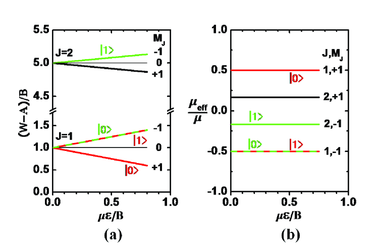
Figure 1: (Color online)Stark states for a polar symmetric top molecule, as functions of $\mu$$\varepsilonup$$/B$. (a) Eigenenergies for $M_{J}=0$ and $\pm 1$ components of $K=1$ levels for $J=1$ and $J=2$ states and (b) corresponding expectation values that determine effective dipole moments, $\mu_{eff}=\langle\text{cos}\rangle$. States used as basis qubits are labeled $|0\rangle$ and $|1\rangle$: type I (green) are $M_{J}=-1$ for $J=2$ and type II (red) are $M_{J}=+1$ and -1 for $J=1$. By virtue of the ordinate scale used, (a) as well as (b) applies to any symmetric top molecule (treated as rigid, without fine or hyperfine structure).

Figure 1 displays for the $K=1$ sublevels of the $J=1$ and 2 symmetric top rotational states the (a) eigenenergies $W=E_{R}+E_{S}$ and (b) expectation values $\langle\text{cos}\rangle=\mu_{eff}/\mu$ for the projection of the dipole moment on the field direction, as functions of $\mu$$\varepsilonup$/$B$. The dependence on $\mu$$\varepsilonup$/$B$ differs markedly from a similar plot for a diatomic molecule (for which $K=0$; cf. Fig. 1 of ref. Wei2 ); there the effective dipole moments are field-dependent and vanish at zero-field. For symmetric top qubit states, to take advantage of the first-order Stark effect, we consider only $K\not=0$ and $M_{J}\not=0$ states. For such states, the effective dipole moments,

$$\mu_{eff}=-\partial E_{S}/\partial\text{\Large$\mathbf{\varepsilonup}$}=\mu M_{J}K/J(J+1)$$ (8)

are just constants independent of the field (except at unusually high fields, where higher order terms become important Stark ). According as $\mu_{eff}$ is positive or negative, the Stark energy drops or climbs as the field strength grows, so the molecular states are termed high field seeking (HFS) or low field seeking LFS), respectively.

II.1 Choice of qubit states

We consider two qualitatively distinct choices for qubit states, designated I and II. The orthodox choice, type I, is exemplified by

$$|0\rangle=|J=1,K=1,M_{J}=-1\rangle\;\;\;\;\;\text{and}\;\;\;\;\;|1\rangle=|J=2,K=1,M_{J}=-1\rangle$$ (9)

For this choice (green curves in Fig. 1), radiation induced transitions between the qubits are fully allowed, in accord with the familiar selection rules, $\triangle J=0,\pm 1$; $\triangle K=0$; $\triangle M=0,\pm 1$ Townes . Also, both the $|0\rangle$ and $|1\rangle$ qubit states are LFS, thereby facilitating trapping by either DC or AC fields or an optical lattice Meerakker . The corresponding eigenenergies, $E_{R}+E_{S}$, are

$$W_{0}=A+B+\frac{\mu\text{\Large$\mathbf{\varepsilonup}$}}{2}\;\;\;\;\;\text{and}\;\;\;\;\;W_{1}=A+5B+\frac{\mu\text{\Large$\mathbf{\varepsilonup}$}}{6}$$ (10)

and the $\text{cos}\theta$ matrix elements are

$$C_{0}=\langle 0|\text{cos}\theta|0\rangle=-\frac{1}{2},\;\;\;\;\;\;\;\;\;\;C_{1}=\langle 1|\text{cos}\theta|1\rangle=-\frac{1}{6},\;\;\;\;\;\;\;\;\;\;C_{X}=\langle 0|\text{cos}\theta|1\rangle=\frac{\sqrt{15}}{10}$$ (11)

We are particularly interested in an unorthodox choice, type II (red curves in Fig. 1). For this, the qubit states are

$$|0\rangle=|J=1,K=1,M_{J}=+1\rangle\;\;\;\;\;\text{and}\;\;\;\;\;|1\rangle=|J=1,K=1,M_{J}=-1\rangle$$ (12)

The eigenenergies are degenerate at zero-field but for $\text{\Large$\mathbf{\varepsilonup}$}>0$ split apart strongly and linearly,

$$W_{0}=A+B-\frac{\mu\text{\Large$\mathbf{\varepsilonup}$}}{2}\;\;\;\;\;\text{and}\;\;\;\;\;W_{1}=A+B+\frac{\mu\text{\Large$\mathbf{\varepsilonup}$}}{2}$$ (13)

and the $\text{cos}\theta$ matrix elements are

$$C_{0}=\langle 0|\text{cos}\theta|0\rangle=\frac{1}{2},\;\;\;\;\;\;\;\;\;\;C_{1}=\langle 1|\text{cos}\theta|1\rangle=-\frac{1}{2},\;\;\;\;\;\;\;\;\;\;C_{X}=\langle 0|\text{cos}\theta|1\rangle=0$$ (14)

These type II qubits render the effective dipole moments constant and equal in magnitude but opposite in sign. However, type II qubits require further specification. As initially defined in Eq.(12), the transition $|0\rangle\leftrightarrow|1\rangle$ between the qubits requires $\triangle M_{J}=\pm 2$. Thus, it is not allowed as a one-photon electric dipole transition (the transition cosine, $C_{X}=0$). It is allowed as a two-photon transition (using the $J=1$, $K=1$, $M_{J}=0$ state as intermediate). Another remedy, simpler to implement, is to use a molecule that contains a nuclear quadrupole moment. Even a small quadrupole coupling constant typically introduces sufficient mixing of Stark states to make $\triangle M_{J}=\pm 2$ transitions become prominent in microwave or radiofrequency spectra Klemperer . In accord with theory Townes ; Coester , in the next subsection we show that modifying the type II qubit choice to exploit the quadrupole hyperfine structure renders $C_{X}\not=0$, enabling $|0\rangle\leftrightarrow|1\rangle$ to occur as a one-photon transition.

In another contrast with type I, for type II qubits $|0\rangle$ is HFS while $|0\rangle$ is LFS. That is also often the case for qubit states considered for diatomic molecules, and is not regarded as a serious handicap Meerakker . Although HFS states are harder to trap, both HFS and LFS can be captured simultaneously in an AC trap or an optical lattice Meerakker .

II.2 Quadrupole perturbation of Stark states

For simplicity, we consider symmetric top molecules having only one atom with a nuclear quadrupole moment, with that atom located on the symmetry axis. We also treat explicitly only cases in which the nuclear spin $I=1$ for that atom, and the quadrupole interaction is much smaller than the Stark energy. The $CH_{3}CN$ molecule Kukolich is a prototypical case: for the ${}^{14}N$ nucleus (spin $I=1$), the quadrupole coupling constant is $eqQ=-4.22\;\text{MHz}$. For conditions in prospect for a quantum computer, usually $\mu$$\varepsilonup$$\;>100\;\text{MHz}$. A first-order perturbation treatment, referred to as the ”strong-field approximation” Townes ; Coester , and governed by the ratio $eqQ/\mu$$\varepsilonup$, hence is appropriate for this example and many others.

When set-up in the usual $|JKM_{J}IM_{I}\rangle$ basis, with $M_{I}$ the projection of the nuclear spin on the $\varepsilonup$-field direction, the Hamiltonian matrix, ${\bf H}_{R}+{\bf H}_{S}+{\bf H}_{Q}$, is diagonal in $J$, $K$, and $I$. The ${\bf H}_{R}$ and ${\bf H}_{S}$ portions are also diagonal in $M_{J}$ and $M_{I}$ whereas ${\bf H}_{Q}$ has off-diagonal elements which connect $M_{J}$ and $M_{I}$ states differing by up to two units. In consequence of the resulting mixing, neither $M_{J}$ nor $M_{I}$ is a ”good” quantum number. Their sum, $M_{J}+M_{I}$ remains good, however, since the total angular momentum along the field must be constant. Accordingly, we modify our choices for the $|0\rangle$ and $|1\rangle$ qubits of Eqs.(9) and (12), that involve $M_{J}=\pm 1$, to specify them further as particular hyperfine components with $M_{J}+M_{I}=0$. In Appendix A we evaluate the contributions from ${\bf H}_{Q}$ to the qubit eigenenergies and cosine matrix elements.

In first-order, the quadrupole interaction simply adds to the qubit eigenvalues of Eq. (10) or (13) a diagonal term given by

$$E_{Q}=eqQ/40\;\;\;\;\;\text{or}\;\;\;\;\;eqQ/56$$ (15)

for $J=1$ or $J=2$, respectively.

The cosine matrix elements of Eqs.(11) and (14) are augmented by terms involving $w=|eqQ|/\mu$$\varepsilonup$, given in Table I. Since typically $w<10^{-2}$, these contributions are insignificant for type I qubits, and for the $C_{0}$ or $C_{1}$ elements for type II qubits, but of major importance in the $C_{X}$ transition element for type II, which would otherwise be zero. Even when $C_{X}$ is very small, conventional power levels suffice to make transitions facile between the $M_{J}=\pm 1$ Stark components Klemperer .

Table 1: Cosine matrix elements for symmetric top qubits^a.

	Type I qubits	Type II qubits
$C_{0}$	$-1/2-0.00168w+0.0418w^{2}$	$1/2-0.00347w-0.0213w^{2}$
$C_{1}$	$-1/6+0.00526w+0.0218w^{2}$	$-1/2-0.00168w+0.0418w^{2}$
$C_{X}$	$\sqrt{15}/10-0.00658w-0.0437w^{2}$	$0+0.153w-0.0108w^{2}$

III TWO INTERACTING DIPOLES

Adding a second trapped polar symmetric top, identical to the first but a distance $r_{12}$ apart, introduces the dipole-dipole coupling interaction,

$$V_{d-d}=\frac{\bm{\mu}_{1}\cdot\bm{\mu}_{2}-3(\bm{\mu}_{1}\cdot{\bf n})(\bm{\mu}_{2}\cdot{\bf n})}{|{\bf r}_{1}-{\bf r}_{2}|^{3}}$$ (16)

Here n denotes a unit vector along ${\bf r}_{12}$. In the presence of an external field, it becomes appropriate to express $V_{d-d}$ in terms of angles related to the field direction (Appendix A in ref. Wei2 ). The result after averaging over azimuthal angles reduces to

$$V_{d-d}=\Omega(1-3\text{cos}^{2}\alpha)\text{cos}\theta_{1}\text{cos}\theta_{2}$$ (17)

where $\Omega=\mu^{2}/r_{12}^{3}$, the angle $\alpha$ is between the ${\bf r}_{12}$ vector and the field direction and polar angles $\theta_{1}$ and $\theta_{2}$ are between the ${\bm{\mu}}_{1}$ and ${\bm{\mu}}_{2}$ dipoles and the field direction.

When set up in a basis of the qubit states (either type I or II) for the pair of molecules, $\{|00\rangle,|01\rangle,|10\rangle,|11\rangle\}$, the $H_{R}+H_{S}$ portion of the Hamiltonian takes the form

$$\left(\begin{array}[]{cccc}W_{0}+W_{0}^{\prime}&0&0&0\\ 0&W_{0}+W_{1}^{\prime}&0&0\\ 0&0&W_{1}+W_{0}^{\prime}&0\\ 0&0&0&W_{1}+W_{1}^{\prime}\end{array}\right)$$ (18)

and the $V_{d-d}$ portion is

$$\Omega_{\alpha}\left(\begin{array}[]{cccc}C_{0}C_{0}^{\prime}&C_{0}C_{X}^{\prime}&C_{X}C_{0}^{\prime}&C_{X}C_{X}^{\prime}\\ C_{0}C_{X}^{\prime}&C_{0}C_{1}^{\prime}&C_{X}C_{X}^{\prime}&C_{X}C_{1}^{\prime}\\ C_{X}C_{0}^{\prime}&C_{X}C_{X}^{\prime}&C_{1}C_{0}^{\prime}&C_{1}C_{X}^{\prime}\\ C_{X}C_{X}^{\prime}&C_{X}C_{1}^{\prime}&C_{1}C_{X}^{\prime}&C_{1}C_{1}^{\prime}\end{array}\right)$$ (19)

where $\Omega_{\alpha}=\Omega(1-3\text{cos}^{2}\alpha)$.The primes attached to quantities for the second dipole indicate that the external field magnitude will differ at its site; that is necessary for addressing the sites and to ensure that the qubit states $|01\rangle$ and $|10\rangle$ differ in energy.

III.1 Evaluating entanglement of eigenstates

The form of the Hamiltonian in Eqs. (18) and (19) is identical to that for two polar diatomic molecules, treated in ref. Wei2 . Thus, we follow the same procedures in evaluating eigenstate properties and entanglement for symmetric tops, merely introducing the appropriate matrix elements for qubits of types I and II (as specified in Sec IIA). We again use unitless reduced variables, $x$ = $\mu$$\varepsilonup$$/B$ and $y=\Omega_{\alpha}/B$; in terms of customary units, these are given by

$$x=\mu\text{\Large$\mathbf{\varepsilonup}$}/B=504\mu(\text{Debye})\text{\Large$\mathbf{\varepsilonup}$}(\text{kV/cm})/B(\text{MHz})$$ (20)

$$y=\Omega_{\alpha}/B=1.51\times 10^{-4}\mu^{2}(\text{Debye})/r^{3}(\mu m)/B(\text{MHz})$$ (21)

Likewise, we use $z=eqQ/B$ for quadrupole coupling terms. The pertinent ranges are $x<1$, $y<10^{-5}$, and $|z|<5\times 10^{-3}$ for candidate symmetric tops (with dipole moments $\mu<4$ D, quadrupole coupling $|eqQ|<10$ MHz, and rotational constants $B>2000$ MHz) under conditions deemed practical for prospective quantum computer designs (field strengths $\varepsilonup$ $<1$ kV/cm, intermolecular spacings $r\sim 0.5\mu m$). Unless otherwise noted, we take $\alpha=90^{o}$. In the pertinent regime, the dependence on $x$, $y$, and $z$ of the eigenenergies is simply linear in all three variables.

Another key variable is $\triangle x=x^{\prime}-x$, specified by the difference in the field strength at adjacent qubit sites. As the site addresses are provided by observing the one-qubit transition, $|0\rangle\leftrightarrow|1\rangle$, the size of $\triangle x$ must be large enough to produce a clearly resolvable Stark shift between the sites. Yet $\triangle x$ must not exceed $X_{R}/N$, where $N$ is the number of sites and $X_{R}$ the range in $x$ of field strengths considered feasible. To benefit from keeping the field strength relatively low, we take $X_{R}\sim 1$; then to accommodate $N$ sites requires $\triangle x<X_{R}/N$. At least for exploratory calculations for up to $N\sim 10^{3}$, we consider $10^{-4}<\triangle x<10^{-2}$ appropriate.

Tables II and III exhibit properties, for qubit types I and II, respectively, of the four eigenstates of the two-dipole system, listed in order of increasing energy ($i=1\rightarrow 4$). The eigenvalues are obtained as simple explicit functions of $x$, $x^{\prime}$, $y$, $z$, applicable to any polar symmetric top molecule and conditions within the pertinent regime specified above. Also indicated, in order of magnitude only, are quantities that express the extent of entanglement among the qubit basis states, but must be evaluated by numerical means. Entanglement is exhibited most directly in the coefficients with which the qubit basis states appear in the eigenfunctions,

$$\Psi_{i}=a_{i}|00\rangle+b_{i}|01\rangle+c_{i}|10\rangle+d_{i}|11\rangle$$ (22)

In Appendix B, we give somewhat cumbersome formulas for these coefficients in terms of $x$, $x^{\prime}$, $y$, $z$. Tables II and III show just orders of magnitude, evaluated for $CH_{3}CN$, under conditions specified in Table IV. This is done to illustrate most simply a major point: In the pertinent range, the entanglement is so feeble that the successive eigenfunctions $\Psi_{i}$ differ only slightly from the respective basis qubits, $\{|00\rangle,|01\rangle,|10\rangle,|11\rangle\}$; there is little admixture with other qubits.

Table 2: Eigenproperties for $N=2$ symmetric top dipoles, type I qubits^a.

$i$	$(E_{i}-2A)/B$	$\Psi_{i}$	$|00\rangle$	$|01\rangle$	$|10\rangle$	$|11\rangle$	$C_{12}$
1	$2+\frac{x}{2}+\frac{x^{\prime}}{2}+\frac{y}{4}+\frac{z}{20}$		$1-O(10^{-15})$	$+O(10^{-8})$	$+O(10^{-8})$	$-O(10^{-8})$	$O(10^{-8})$
2	$6+\frac{x}{2}+\frac{x^{\prime}}{6}+\frac{y}{12}+\frac{3z}{70}$		$-O(10^{-8})$	$1-O(10^{-7})$	$-0.0009$	$+O(10^{-8})$	$0.0018$
3	$6+\frac{x^{\prime}}{2}+\frac{x}{6}+\frac{y}{12}+\frac{3z}{70}$		$-O(10^{-8})$	$-0.0009$	$1-O(10^{-7})$	$+O(10^{-8})$	$0.0018$
4	$10+\frac{x}{6}+\frac{x^{\prime}}{6}+\frac{y}{36}+\frac{z}{28}$		$+O(10^{-8})$	$-O(10^{-8})$	$-O(10^{-8})$	$1-O(10^{-15})$	$O(10^{-8})$

Table 3: Eigenproperties for $N=2$ symmetric top dipoles, type II qubits^a.

$i$	$(E_{i}-2A)/B$	$\Psi_{i}$	$|00\rangle$	$|01\rangle$	$|10\rangle$	$|11\rangle$	$C_{12}$
1	$2-\frac{x}{2}-\frac{x^{\prime}}{2}+\frac{y}{4}+\frac{z}{20}$		$1-O(10^{-17})$	$-O(10^{-9})$	$-O(10^{-9})$	$-O(10^{-12})$	$O(10^{-12})$
2	$2+\frac{x}{2}-\frac{x^{\prime}}{2}-\frac{y}{4}+\frac{z}{20}$		$+O(10^{-9})$	$1-O(10^{-17})$	$-O(10^{-10})$	$+O(10^{-9})$	$O(10^{-9})$
3	$2+\frac{x^{\prime}}{2}-\frac{x}{2}-\frac{y}{4}+\frac{z}{20}$		$+O(10^{-9})$	$+O(10^{-10})$	$1-O(10^{-17})$	$+O(10^{-9})$	$O(10^{-9})$
4	$2+\frac{x}{2}+\frac{x^{\prime}}{2}+\frac{y}{4}+\frac{z}{20}$		$+O(10^{-12})$	$-O(10^{-9})$	$-O(10^{-9})$	$1-O(10^{-17})$	$O(10^{-12})$

Table 4: Parameters for $CH_{3}CN$ molecule.

Properties		Reduced variables
$\mu$	3.92 D	$x=\mu$$\varepsilonup$$/B=0.0107$
$B$	9198.8 MHz	$\triangle x=\mu$($\varepsilonup$′-$\varepsilonup$)$/B=10^{-3}$
$eqQ$	-4.22 MHz	$y=\Omega_{\alpha}/B=2\times 10^{-6}$
$\mu$$\varepsilonup$	988 MHz	$z=eqQ/B=4.6\times 10^{-4}$
$\Omega_{\alpha}$	18.5 kHz	$w=|eqQ|/\mu$$\varepsilonup$ = $4.3\times 10^{-3}$

III.2 Pairwise concurrence of eigenstates

A quantitative measure of entanglement is provided by the pairwise concurrence function, $C_{12}$, which becomes unity when entanglement is maximal and zero when it is entirely lacking. The general prescription for evaluating $C_{12}$ involves somewhat arcane manipulations of the density matrix Wootters . However, it becomes simple here as the entanglement arises entirely from off-diagonal terms in the $V_{d-d}$ matrix of Eq.(19). These terms are small, since they are all proportional to $y$, which is $<10^{-5}$. Otherwise the off-diagonal terms contain either $C_{X}$, or $C_{X}^{2}$, factors essentially independent of $x$ or $x^{\prime}$; for type I qubits, $C_{X}\sim 0.4$ and for type II qubits $C_{X}<10^{-3}$. Accordingly, as seen in Tables II and III, the ground eigenstate, $\Psi_{1}$, and the highest excited eigenstate, $\Psi_{4}$, are almost solely composed of the basis qubits $|00\rangle$ and $|11\rangle$, respectively, especially for type II. In terms of the coefficients in Eq.(22), in this case $C_{12}$ is to good approximation just $2d_{1}$ or $2a_{4}$, for eigenstates 1 and 4, respectively. Thus, for eigenstates 1 and 4, we find

$$C_{12}=K(x,x^{\prime})[\Omega_{\alpha}/B]$$ (23)

with weak dependence on $x$, given by

$$K(x)=0.03752+0.00312x+0.00029x^{2}$$ (24)

and the dependence on $x^{\prime}$ is well represented by $K(x,x^{\prime})=\left[K(x)K(x^{\prime})\right]^{1/2}$ when $\triangle x=x^{\prime}-x<10^{-2}$. The concurrence for a pair of polar diatomic molecules Wei2 has this same form (for small $\Omega_{\alpha}/B$), but the second-order Stark effect makes the $K(x)$ coefficient much larger ($>0.12$ for $x<1$).

The $C_{12}$ function becomes more interesting for the middle eigenstates, $\Psi_{2}$ and $\Psi_{3}$. As seen in Tables II and III, for the conditions we refer to as ”pertinent” these eigenstates are essentially just the $|01\rangle$ and $|10\rangle$ basis qubits, respectively. However, if $\triangle x\rightarrow 0$, the eigenenergies $E_{2}$ and $E_{3}$ become the same. In that limit, even very small $y$ can produce strong entanglement of the $|01\rangle$ and $|10\rangle$ qubits. Figure 2 illustrates how $C_{12}$ varies as $\triangle x$ is scanned over a range from well below to well above $y$; at least in principle that can be done by adjusting the $\varepsilonup$-field and$/$or the spacing of the dipoles. The curve shown is given by

$$C_{12}=2|\alpha_{\pm}|/(1+\alpha_{\pm}^{2})$$ (25)

with

$$\alpha_{\pm}=\frac{(E_{3}-E_{2})\pm\left[(E_{3}-E_{2})^{2}+4\triangle^{2}\right]^{1/2}}{2\triangle}$$ (26)

where $\triangle=C_{X}^{2}\Omega_{\alpha}$. This formula for $C_{12}$ results from omitting all off-diagonal terms in the $V_{d-d}$ matrix except the pair that couple $|01\rangle$ and $|10\rangle$ along the antidiagonal. The eigenstates then become $\Psi_{2}=\Psi_{+}$ and $\Psi_{3}=\Psi_{-}$, with

$$\Psi_{\pm}=\frac{|10\rangle-\alpha_{\pm}|01\rangle}{\sqrt{1+\alpha_{\pm}^{2}}}$$ (27)

In the limit $E_{3}-E_{2}\ll\triangle$ (i.e, $\triangle x\ll y$), where $\alpha_{\pm}\rightarrow\pm 1$ and $C_{12}\rightarrow 1$, the eigenfunctions become maximally entangled states, termed Bell states. Figure 2 also displays points obtained from numerical diagonalization of the Hamiltonian with all elements included in the $V_{d-d}$ matrix. For both type I (green points) and type II (red points), the numerical results agree very closely with the formula given in Eq.(25). It is a striking demonstration of the extent to which matrix elements that connect almost degenerate levels generate entanglement.

III.3 Inducing large entanglement via resonant pulses

Under the ultracold conditions needed to localize trapped molecules in the qubit sites, the two-dipole system is in its ground eigenstate, $\Psi_{1}\sim|00\rangle$, wherein the entanglement is very small. However, the large entanglement often needed for quantum computing can be induced dynamically via resonant pulses to higher eigenstates Jones2 ; Thanks . Several procedures have been presented for accomplishing this to use polar molecules in operating quantum logic gates andre ; yelin ; Charron ; kuz ; lics ; YelinDeMille ; Shioya ; Mishima ; Chen ; Reina ; Sugny . Here we consider just a rudimentary version, exemplified with the CNOT gate, since our chief aim is to compare and contrast the symmetric top qubits of types I and II with the diatomic case treated in ref. Wei2 .

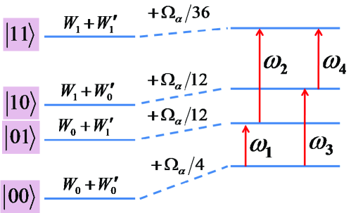
Figure 3: (Color online) Schematic energy levels for type I qubit eigenstates of two symmetric top dipoles. At left are indicated qubit basis states, with corresponding eigenenergies from Eqs.(18) and (19). Contributions from quadrupole coupling are not shown (but included in Tables II and V). At right are transitions that are involved in CNOT operation: $\omega_{1}$ transfers the dipole at site 2 from $|0\rangle$ to $|1\rangle$, with dipole at site 1 remaining in $|0\rangle$, then 2 transfers dipole at site 1 from $|0\rangle$ to $|1\rangle$ with dipole at site 2 remaining in $|1\rangle$. The same result could be reached by $\omega_{3}$ followed by $\omega_{4}$. Transition frequencies are given in Table V.

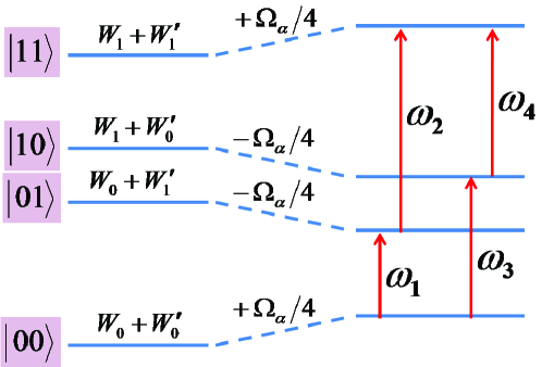
Figure 4: (Color online) Schematic energy levels for type II qubit eigenstates of two symmetric top dipoles; format as in Fig. 3. Eigenenergies, including quadrupole coupling are (not shown) are given in Tables III and transition frequencies in Table V.

Figures 3 and 4 give schematic diagrams, analogous to Fig. 10 of ref. Wei2 , depicting available transitions among the two-dipole eigenstates. Table V lists the corresponding transition frequencies. In contrast to type I, for type II qubits the contributions from both the rotational constants and quadrupole coupling cancel out, hence the transition frequencies depend only on the Stark energy shifts and dipole-dipole interaction. Since the entanglement is so feeble for the eigenstates, as seen in Tables II and III, for a heuristic description we may speak as if the transitions simply occur between the unperturbed basis qubits. A typical procedure applies a $\pi/2$ pulse resonant with the transition frequency $\omega_{1}$ to transfer population from the ground eigenstate $|00\rangle$ to the excited state $|01\rangle$, thereby putting the system into the state $2^{-1/2}(|00\rangle+|01\rangle)$. Then a $\pi$ pulse resonant with the transition $\omega_{2}$ between $|01\rangle$ and $|11\rangle$ will put the system into the state $2^{-1/2}(|00\rangle+|11\rangle)$, which is a completely entangled Bell state. The same process can be done applying a $\pi/2$ pulse to $\omega_{3}$, followed by a $\pi$ pulse to $\omega_{4}$.

Table 5: Transition frequencies between eigenstates of two dipoles^a.

	Type I qubits	Type II qubits
$\omega_{1}/B$	$4-x^{\prime}/3-y/6-z/140$	$x-y/2$
$\omega_{2}/B$	$4-x/3-y/18-z/140$	$x^{\prime}+y/2$
$\omega_{3}/B$	$4-x/3-y/6-z/140$	$x^{\prime}-y/2$
$\omega_{4}/B$	$4-x^{\prime}/3-y/18-z/140$	$x+y/2$
$\triangle\omega/B$	$y/9$	$y$

To carry out such procedures, the transition frequencies need to be unambiguously resolved from each other. As evident in Table V, for both type I and II qubits, $\omega_{1}$ can be resolved from $\omega_{2}$ and $\omega_{3}$ from $\omega_{4}$ simply by adjusting the difference in external field strengths, $\triangle x=x^{\prime}-x$. In frequency units, a Stark shift of $\triangle x=10^{-3}$ for $CH_{3}CN$ is 3 MHz for type I qubits and 9 MHz for type II. The relative difference is far more in favor of type II, because $\omega_{1}=35,869$ MHz for type I whereas it is only 988 MHz for type II. However, for either type such differences are easily resolvable in conventional microwave and radiofrequency spectroscopy.

Resolving $\omega_{1}$ from $\omega_{4}$ and $\omega_{2}$ from $\omega_{3}$ presents an experimental challenge. The frequency difference is governed simply by the dipole-dipole interaction, since

$$\triangle\omega=\omega_{4}-\omega_{1}=\omega_{2}-\omega_{3}=\Omega_{\alpha}(C_{1}-C_{0})(C^{\prime}_{1}-C^{\prime}_{0})$$ (28)

The $\triangle\omega$ shift is the essential feature of a CNOT gate: $\omega_{3}$ transfers the target qubit on dipole 1 from $|0\rangle$ to $|1\rangle$ when the control qubit on dipole 2 is in $|0\rangle$, whereas $\omega_{2}=\omega_{3}-\triangle\omega$ transfers the target from $|0\rangle$ to $|1\rangle$ when the control is in $|1\rangle$. For $\omega_{1}$ and $\omega_{4}$ the roles of target and control sites are exchanged. Unlike the diatomic case Wei2 , for symmetric tops the cosine elements are nearly independent of the external field in the pertinent regime, except via the minor quadrupole terms included in Table I. Thus,

$$\triangle\omega=\Omega_{\alpha}/9\;\;\;\;\;\text{for type I and}\;\;\;\;\;\triangle\omega=\Omega_{\alpha}\;\;\;\;\;\text{for type II}$$ (29)

Here the significant advantage of type II occurs because both $C_{0}$ and $C_{1}$ are large and of opposite sign. In frequency units, for $CH_{3}CN$ the $\triangle\omega$ shift is only 2 kHz for type I and 18 kHz for type II. Again, the relative difference greatly favors type II, since $\triangle\omega/\omega_{1}$ is more than a hundredfold larger than for type I.

As compared with candidate polar diatomic molecules Wei2 , we expect prospects for resolving $\triangle\omega$ for symmetric tops are improved in two ways: (1) The first-order Stark effect enables use of a much less strong external field. That should reduce line broadening caused by nonuniformity and fringing of the electric field. (2) The choice of Stark components for type II qubits lowers the transition frequencies between qubit states down to the radiofrequency range (often factors of 30-50 lower than transitions between rotational states, which occur in the microwave range). In molecular beam spectra, collision free but without trapping in an optical lattice, line widths are typically much smaller in the rf region; e.g., 2 kHz or below for $\triangle J=0$, $\triangle M_{J}=\pm 1$ transitions Klemperer . The effect of the optical lattice on line widths is uncertain. It may introduce broadening via motional shifts, which are strongly dependent on the well depths required for trapping Barker . Such shifts have been avoided for ultracold atoms by use of ”magic” optical trapping conditions Zelevinsky , but there might be less scope to do that for molecules. As yet, no line width data have been reported for ultracold molecules trapped in an optical lattice and subject to a sizable electric field. Thus, although less problematic for type II symmetric top qubits, the feasibility of resolving the $\triangle\omega$ shift remains an open question.

III.4 Comparison with NMR

A motivation for considering symmetric top type II qubits is the resemblance to spin-1/2 NMR, which has been extensively analyzed in the context of quantum computation Cory ; Cory2 ; Cory3 ; Vandersypen ; Price ; Price2 . The resemblance stems from the unorthodox choice of $\pm M_{J}$ Stark components for type II qubits. That renders the effective qubit dipole moments, $\mu_{eff}=\mu\langle\text{cos}\theta\rangle$, which are essentially independent of the external field, equal in size but opposite in spatial orientation. There are further similarities. For the generic $N=2$ case, the corresponding Hamiltonian for NMR resembles our Eqs. (18) plus (19), except for omission of the rotational energy. The molecular dipoles are replaced by nuclear spins, the Stark field by a Zeeman field, and the dipole-dipole interaction by spin-spin coupling. Thereby our $\Omega_{\alpha}$ is replaced by $J_{12}$, the spin-spin coupling parameter. Since the Zeeman energy terms are much larger than the spin-spin coupling, the equivalent of our $V_{d-d}$ matrix is usually approximated as simply diagonal Cory2 . Accordingly, the eigenstates are then just the basis qubits $\{|00\rangle,|01\rangle,|10\rangle,|11\rangle\}$, so entirely lack entanglement. That resembles our type II qubits when $C_{X}=0$, in the absence of quadrupole coupling.

Another, different sort of similarity arises from the choice of NMR qubits as nuclear spins on different atoms within a molecule Vandersypen . Even for atoms of the same kind, chemical shifts cause the effective external magnetic field to differ at different sites. This corresponds to the role of the gradient in electric field, emphasized in Sec.III, wherein $\triangle x>0$ is important both for addressing sites and for resolving the $|01\rangle$ and $|10\rangle$ qubit pairs.

Many procedures for producing dynamical entanglement in NMR systems by means of sequences of radiofrequency pulses have been developed and demonstrated in performing quantum gates and algorithms Cory ; Cory2 ; Cory3 ; Vandersypen ; Price ; Price2 . The prospects for adapting some of these to polar symmetric tops invite systematic study. We will not pursue that here, but mention an example pertinent to resolving $\triangle\omega$, the key frequency shift for implementing the CNOT gate. For NMR the analog of our Eq.(28) holds, with $\triangle\omega=J_{12}$.

Even if $\triangle\omega$ is too small to be well resolved, another general way to perform a CNOT gate has been demonstrated in a NMR spin system Price2 . Because qubits in both sites 1 and 2 are in superposition states of $|0\rangle$ and $|1\rangle$, the qubit at site 1 comprises two populations, one coupled to the qubit at site 2 in the $|0\rangle$ state and the other to the $|1\rangle$ state there. By means of a $\pi/2$ pulse, the qubit at site 1 can be rotated into the transverse plane, where both populations will undergo Larmor precession, but with different frequencies. After a time $\sim 1/\triangle\omega$, the two populations are $180^{o}$ out of phase. Then another $\pi/2$ pulse can be performed to place both populations at site 1 along the z-axis. The net effect is to complete a CNOT gate with the qubit at site 2 controlling that at site 1. At least in principle, such procedures, well developed in NMR, seem applicable to symmetric top type II qubit states.

IV CONCLUSIONS AND PROSPECTS

The seminal proposal by DeMille Demille envisioned a quantum computer using as qubits rotational states of ultracold polar molecules, trapped in an optical lattice, partially oriented in an external electric field and coupled by dipole-dipole interactions. Many aspects and variants have been extensively studied in the decade since, all considering diatomic molecules Micheli ; Charron ; kuz ; ni ; lics ; YelinDeMille ; Wei1 ; Wei2 . As the external field has an essential role, the fact that the Stark effect is second-order for diatomic molecules has major consequences. The field strength must be sufficiently high to induce extensive hybridization of rotational states, so that the molecules undergo pendular oscillations about the field direction; otherwise rotational tumbling averages out the effective dipole moments in the laboratory frame. As discussed in Sec. IIIC, and more fully in ref. Wei2 , line broadening by the high field handicaps resolution of $\triangle\omega$, the key frequency shift for 2-qubit operations.

We find that polar symmetric top molecules offer significant advantages. These come primarily from the first-order Stark effect, available for all states with $K$ and $M_{J}$ nonzero. As symmetric tops in those states precess rather than tumble, the effective dipole moments are independent of the electric field strength (except at high fields). Because there is no need to induce pendular hybridization, a considerably lower external field can be used, thereby improving prospects for resolving the $\triangle\omega$ shift. Moreover, in the first-order Stark effect the $\pm M_{J}$ components are readily resolved (not possible for second-order). This enabled considering the $|J=1,K=1,M_{J}=\pm 1\rangle$ Stark components as the basis qubits (our type II), rather than rotational states (type I). That lowers the transition frequencies between eigenstates (cf. Table V) to the radiofrequency range, again more congenial for resolving the $\triangle\omega$ shift. Even more welcome, the use of $\pm M_{J}$ components as qubits brings forth direct correspondences with spin-1/2 NMR systems. This opens up the prospect of exploiting with symmetric tops a wide repertoire of radiofrequency NMR techniques developed for quantum information processing.

Another prospect for dealing with the small size of the $\triangle\omega$ shift involves spatial rather than frequency resolution. This is exemplified by quantum computer designs employing superconducting flux qubits Groot . For these, the generic $N=2$ Hamiltonian in the case of transversely coupled qubits is much like our Eqs.(18) and (19). Instead of the Stark terms, $\mu$$\varepsilonup$ and $\mu$$\varepsilonup$^′, there appear single-qubit energy splittings, denoted $\triangle_{1}$ and $\triangle_{2}$, respectively, and in place of $\Omega_{\alpha}$ there appears the qubit-qubit coupling energy, denoted by $\mathfrak{J}$ (unrelated to rotational angular momentum or NMR spin-spin). The analog of our $V_{d-d}$ matrix has nonzero elements only along the anti-diagonal (equivalent to setting our $C_{0}$ and $C_{1}=0$). However, for typical conditions, $\mathfrak{J}<<(\triangle_{1}-\triangle_{2})$, the analog reduces just to the simple case described under our Eq.(26) and Fig. 2; the correspondence replaces our $C_{X}^{2}\Omega/(E_{3}-E_{2})$ by $\mathfrak{J}/(\triangle_{1}-\triangle_{2})$. The transitions involved in the CNOT gate (cf. Fig. 1b of ref. Groot ) then occur in degenerate pairs, $\omega_{1}=\omega_{4}$ and $\omega_{2}=\omega_{3}$. Therefore, $\triangle\omega=0$, so frequency-selective operations are impossible. Yet, one transition of each degenerate pair can be selectively suppressed while coherently exciting the other, ”by simultaneously driving both qubits with the resonant frequency of that pair, employing different amplitudes and phases” Groot . This method requires spatial resolution sufficient to enable qubits on different sites to be driven individually. That may not be feasible for our conditions, with polar molecules separated by only 0.5 $\mu$m. Such a method is well suited to a proposed design with molecules trapped in QED cavities spaced $\sim 1$ cm (!) apart along a superconducting transmission line resonator andre .

As in our previous study of entanglement of polar diatomic molecules Wei2 , we provide a generic formulation in terms of reduced variables $(x,\triangle x,y,z,w)$. This makes our results applicable to a broad class of symmetric top molecules and range of conditions envisioned for proposed quantum computers. We also present specific results for the $CH_{3}CN$ molecule Kukolich , regarded as a particularly suitable candidate, particularly for type II qubits. Its large dipole moment enhances the dipole-dipole interaction and hence the $\triangle\omega$ shift, and its nitrogen atom supplies a quadrupole moment that makes the transition dipole $C_{X}$ nonzero, thereby enabling $\triangle M_{J}=\pm 2$ transitions between the type II qubits.

Many aspects important for quantum computing with polar molecules are not discussed here (trapping operations, sources of decoherence, and much more) because extensive analysis given for diatomic molecules Lee ; andre ; yelin ; carr ; Micheli ; Charron ; kuz ; ni ; lics ; YelinDeMille ; Wei1 ; Wei2 pertains as well to symmetric tops. We note an ironic exception. Auxiliary storage qubits are sometimes desired to minimize decoherence or to remove unwanted information Cory2 . Also, ”switchable dipole” schemes have been devised to in effect turn dipole-dipole coupling ”on” or ”off” by transferring qubits between states with very different dipole moments. For diatomic molecules, such maneuvers typically involve excited electronic states; a prototype proposal yelin uses CO, for which the dipole moment in the ground $X^{1}\sum^{+}$ state is only 0.1 D, but in the metastable excited $a^{3}\prod$ state is 1.5 D. For a symmetric top, such things can be accomplished more simply by transfer to states with $K$ or $M_{J}$ zero, where the first-order Stark effect vanishes. For example, in the $J=1$, $K=1$ states of $CH_{3}CN$ under the conditions of Table IV, for $M_{J}=0$ the second-order Stark effect Stark yields an effective dipole moment of only 0.084 D, whereas for $M_{J}=\pm 1$ the first order Stark effect gives an effective moment of 1.96 D. A transfer $M_{J}=\pm 1\rightarrow 0$, without change in the electric field strength, would reduce the dipole-dipole coupling 500-fold.

Symmetric tops offer many other options for qubits. Some, such as hyperfine structure, are also available with diatomic molecules. Others are not, such as doublet structures Weber produced by tunneling through barriers to inversion (e.g., in $NH_{3}$) or internal rotation (e.g., in $CH_{3}CF_{3}$). If inversion is fast ($\sim 1$ Hz for $NH_{3}$ in ground state), the dipole flips rapidly and the Stark effect is second-order, whereas if inversion is slow (e.g. $\sim 1$ year for $AsH_{3}$), it is first-order. For internal rotation involving a three-fold barrier, the tunneling doublets occur as a nondegenerate A state, and a doubly degenerate E state; the Stark effect for A is second- order, for E first-order.

For both diatomic and symmetric top molecules, under conditions considered amenable for proposed quantum computers, the entanglement of eigenstates and the associated pairwise concurrences are very small. Furthermore, it is not needed in the eigenstates, because the entanglement required for computations is actually induced dynamically. The role of dipole-dipole coupling as the source of eigenstate entanglement, via the off-diagonal terms of Eq.(19), therefore is irrelevant. Its important role is determining a different eigenstate property, the $\triangle\omega$ shift, via Eq.(28). The evaluation of $\triangle\omega$ does not require eigenfunctions, only eigenvalues. This is a liberating perspective in considering analysis of multidipole systems well beyond $N=2$.

Mindful of the somewhat metaphysical status often accorded to entanglement Kaiser , we mention that fundamental theory shows that even for symmetric tops, the ”true molecular eigenstates should not have first-order Stark effects” Klemperer2 . That is because the full permutation-inversion group for a molecule shows that the only levels allowed by quantum statistics are nondegenerate. Yet both theory and experiment confirm that a quasi-first-order Stark effect does appear in the presence of even a very weak field ($<$ 0.3 V/cm) that introduces coupling between nearly degenerate states. Hence, the very existence of first-order Stark effect in molecules comes from field-induced entanglement.

APPENDIX A: QUADRUPOLE COUPLING

As outlined in Sec.IIB, we use the ”strong-field” approximation Townes ; Coester , appropriate when the Stark shifts are much larger than hyperfine splittings introduced by quadrupole coupling. We need to evaluate contributions from ${\bf H}_{Q}$ to be added to the qubit eigenvalues of Eqs.(10) and (13). Also, we need to obtain, by diagonalizing ${\bf H}_{S}+{\bf H}_{Q}$, the modified qubit eigenfunctions that arise from mixing of the $M_{J}$ Stark components with the $M_{I}$ nuclear spin components. These are required to determine the quadrupole contributions to the cosine elements of Table I. The requisite matrix elements of the ${\bf H}_{Q}$ Hamiltonian,

$$\langle J,K,I,M_{J},M_{I}|{\bf H}_{Q}|J,K,I,M^{\prime}_{J},M^{\prime}_{I}\rangle$$ (A1)

are given in Eq.(33) of ref. Coester . All contain a common factor,

$$P(J,K,I)=\frac{eqQ}{4(2J-1)(2J+3)(2I-1)}\left(\frac{3K^{2}}{J(J+1)}-1\right)$$ (A2)

For the qubit states we consider,

$$P(1,1,1)=eqQ/40\;\;\;\;\;\text{and}\;\;\;\;\;P(2,1,1)=-eqQ/168$$ (A3)

The elements of ${\bf H}_{Q}$ comprise a $9\times 9$ matrix labeled with $M_{J}=1,0,-1$ and $M_{I}=1,0,-1$. The first order energy of the quadrupole hyperfine components is given by the diagonal elements,

$$E_{Q}=P(J,K,I)\left[3M_{J}^{2}-J(J+1)\right]\left[3M_{I}^{2}-I(I+1)\right]$$ (A4)

Because the sum $M_{F}=M_{J}+M_{I}$ is a good quantum number, the matrix is block diagonal, with five submatrices corresponding to $M_{F}=2,1,0,-1,-2$ (respectively $1\times 1$, $2\times 2$, $3\times 3$, $2\times 2$, $1\times 1$). We deal only with the $M_{F}=0$ block, containing elements connecting the $(M_{J},M_{I})=+1,-1;0,0;\text{and}-1,+1$ hyperfine components:

$$P(1,1,1)\left(\begin{array}[]{ccc}1&-3&6\\ -3&4&-3\\ 6&-3&1\end{array}\right)$$ (A5)

$$P(2,1,1)\left(\begin{array}[]{ccc}-1&-\sqrt{3}&6\\ -\sqrt{3}&4&-\sqrt{3}\\ 6&-\sqrt{3}&-1\end{array}\right)$$ (A6)

To the diagonal elements of these matrices, we add the Stark components, from Eq.(6), $E_{S}=-(\mu$$\varepsilonup$$/J(J+1))M_{J}$, then carry out diagonalization to obtain the $M_{F}=0$ eigenfunctions. As specifying $M_{J}$ automatically specifies $M_{I}$, we denote the eigenfunctions simply by $\Psi(J,\tilde{M}_{J})$, expressed as linear combinations of the basis functions $\phi(J,M_{J})$. Here we revert to wavefunction notation, to avoid confusion with the bra notation used for qubits. Also in labeling the eigenfunctions, we adorn $\tilde{M}_{J}$ with a tilde, to indicate it is no longer a good quantum numbers because the Stark and spin states are mixed. Performing numerical diagonalizations led to recognition that, for $\mu$$\varepsilonup$$\gg eqQ$, the eigenfunctions are well approximated using for each $J$ a single mixing coefficient; for $J=1$:

$$\Psi(1,-\tilde{1})\approx(1-a^{2})\phi(1,-1)-a\phi(1,0)+a\phi(1,+1)$$ (A7)

$$\Psi(1,\tilde{0})\approx a\phi(1,-1)+(1-a^{2})\phi(1,0)-a\phi(1,+1)$$ (A8)

$$\Psi(1,+\tilde{1})\approx-a\phi(1,-1)+a\phi(1,0)+(1-a^{2})\phi(1,+1)$$ (A9)

and for $J=2$:

$$\Psi(2,-\tilde{1})\approx(1-2b^{2})\phi(2,-1)+b\phi(2,0)-\sqrt{3}b\phi(2,+1)$$ (A10)

$$\Psi(2,\tilde{0})\approx-b\phi(2,-1)+(1-b^{2})\phi(2,0)+b\phi(2,+1)$$ (A11)

$$\Psi(2,+\tilde{1})\approx\sqrt{3}b\phi(2,-1)-b\phi(2,0)+(1-2b^{2})\phi(2,+1)$$ (A12)

The coefficients $a$ and $b$ are small positive numbers, determined by $w=|eqQ|/\mu$$\varepsilonup$. From our numerical results, we find

$$a=0.1522w\;\;\;\;\;\text{and}\;\;\;\;\;b=0.1789w$$ (A13)

These values are accurate within 1% for $w<0.1$. Since $M_{J}=\pm 1$ for our qubit states, as defined in Eqs.(9) and (12), we now specify them further as the hyperfine components $\Psi(J,-1)$ and $\Psi(J,+1)$; thus for type I,

$$|0\rangle=|J=1,M_{J}=-1,M_{I}=+1\rangle\;\;\;\;\;\text{and}\;\;\;\;\;|1\rangle=|J=2,M_{J}=-1,M_{I}=+1\rangle$$ (A14)

and for type II,

$$|0\rangle=|J=1,M_{J}=+1,M_{I}=-1\rangle\;\;\;\;\;\text{and}\;\;\;\;\;|1\rangle=|J=1,M_{J}=-1,M_{I}=+1\rangle$$ (A15)

The quadrupole terms in the cosine elements of Table I result from using the mixing coefficients of Eq.(A13) with Eqs.(A7) and (A10) for type I qubits and Eqs.(A7) and (A9) for type II together with Eq.(7) of Sec.II. In particular, for type II this gives $C_{X}\approx a(1-a^{2})$.

Symmetric top molecules, other than $CH_{3}CN$, which contain one nucleus with spin $I=1$ on the symmetry axis, include: $NH_{3}$ and $NF_{3}$, where ${}^{14}N$ has $eqQ=-4.09$ MHz and 7.07 MHz, respectively Kurolich ; Sheridan ; and $CH_{3}D$ and $CF_{3}D$, where ${}^{2}D$ has $eqQ=191$ kHz and 171 kHz, respectively Klemperer ; Kukolich2 . In many halide molecules, such as $CH_{3}X$, the halogen nuclei have $I>1$ and large quadrupole coupling constants Townes . Treatment of such cases requires use of an intermediate or weak-field approximation Coester ; Buckinghama .

APPENDIX B: ENTANGLEMENT OF TWO DIPOLES

For the ranges of reduced variables specified in Sec. III: $x<1$; $10^{-4}<\triangle x<10^{-2}$; $y<10^{-5}$; $|z|<5\times 10^{-3}$; $w<0.1$, we have obtained explicit formulas for the coefficients of the basis qubits in Eq.(22), $\{a_{i},b_{i},c_{i},d_{i}\}$, that determine the two-dipole eigenstate entanglements. Tables VI and VII give these formulas for types I and II qubits, respectively. Also included are corresponding values of the pairwise concurrence, $C_{12}$, for the eigenstates; these conform well to the approximations of Eqs.(25) and (27). The corresponding eigenvalues and orders-of-magnitide of the coefficients, under conditions listed in Table IV, are in Tables II and III. Contributions from quadrupole coupling are not included in Table VI because these only slightly affect the entanglement for type I qubits. The quadrupole contributions are included in Table VII because for type II qubits these are the sole source of eigenvalue entanglement (since without them $C_{X}=0$ and the $V_{d-d}$ matrix of Eq.(19) is diagonal). The quadrupole contributions enter the entanglement coefficients in various powers of the ratio of the quadrupole coupling to the Stark energy, $w^{n}$, ranging from $n=2$ to 4. In the concurrence values, the same dependence on $w^{n}$ appears.

Tables VI and VII both pertain to the regime $\triangle x\gg y$, where the Stark shift between adjacent qubit sites is much larger than the dipole-dipole interaction. At present, this regime appears most relevant for implementation prospects. As illustrated in Fig. 2 and Eq.(27), therein the eigenfunctions differ little from the basis qubit states, and entanglement is slight. The extreme opposite limit, $\triangle x=0$, has been analyzed in ref. Charron ; there the eigenfunctions $\Psi_{2}$ and $\Psi_{3}$ become the maximally entangled Bell states, $2^{-1/2}(|01\rangle\pm|10\rangle)$. An interesting consequence emerged. For operation of the CNOT gate, it was concluded that a preliminary pulse of bandwidth much wider than the dipole-dipole interaction should be applied. It would entirely undo the entanglement by forming $\pm$ combinations of the Bell states and thereby unwed the $|01\rangle$ and $|10\rangle$ qubits.

Table 6: Eigenfunction entanglement coefficients, type I qubits^a

$\Psi_{i}=a_{i}|00\rangle+b_{i}|01\rangle+c_{i}|10\rangle+d_{i}|11\rangle$

$a_{1}=(0.07y)^{2}/2$;              $b_{1}=c_{1}=(0.048+0.0044x)y$;

$d_{1}=-a_{4}=(0.019+0.0017x)y$;      $C_{12}=K(x,x^{\prime})y\approx 2d_{1}$;

$a_{2}=-(0.028+0.0026x)y$;       $b_{2}=1-c_{2}^{2}/2$;       $c_{2}=-0.454y/\triangle x$;

$d_{2}=(0.009+0.0009x)y$;      $C_{12}\approx 2|c_{2}|$;

$a_{3}=-(0.062+0.0058x)y$;         $b_{3}=-c_{2}=0.454y/\triangle x$;      $c_{3}=b_{2}$;

$d_{3}=(0.021+0.0019x)y$;      $C_{12}\approx 2|c_{2}|$;

$a_{4}=-d_{1}=(0.019+0.0017x)y$;      $b_{4}=c_{4}=-(0.016+0.0015x)y$;

$d_{4}=-a_{4}=1-(0.04y)^{2}/2$;      $C_{12}=K(x,x^{\prime})y\approx 2a_{4}$;

Table 7: Eigenfunction entanglement coefficients, type II qubits^a

$\Psi_{i}=a_{i}|00\rangle+b_{i}|01\rangle+c_{i}|10\rangle+d_{i}|11\rangle$

$a_{1}=1-b_{1}^{2}$;                               $b_{1}=c_{1}=-0.0786w^{2}y/z$;

$d_{1}=-0.0118w^{3}y/z$;            $C_{12}=0.0247w^{3}y/z\approx 2d_{1}$;

$a_{2}=d_{2}=a_{3}=d_{3}=0.0743w^{2}y/z$;        $b_{2}=-c_{3}=-0.0225w^{2}y/\triangle x$;

$c_{2}=1-a_{2}^{2}$;      $d_{2}=a_{2}$;      $C_{12}=0.044w^{2}y/\triangle x\approx 2|b_{2}|$;

$a_{3}=d_{3}=a_{2}=d_{2}$;      $b_{3}=c_{2}=1-a_{2}^{2}$;      $c_{3}=-b_{2}=0.0225w^{2}y/\triangle x$;

$d_{3}=a_{3}$;                  $C_{12}=0.044w^{2}y/\triangle x\approx 2|c_{3}|$;

$a_{4}=0.0107w^{3}y/z$;                     $b_{4}=c_{4}=-0.0715w^{2}y/z$;

$d_{4}=1-b_{4}^{2}$;                  $C_{12}=0.0205w^{3}y/z\approx 2a_{4}$;

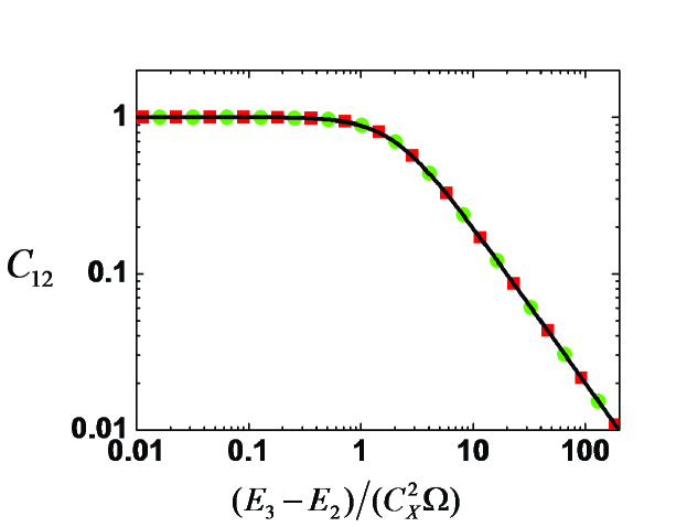
Figure 2: (Color online) Pairwise concurrence $C_{12}$ for eigenstates 2 and 3 of two symmetric top dipoles entangled via dipole-dipole interaction, as a function of the ratio of the difference of the eigenvalues, $(E_{3}-E_{2})$, to the element, $C_{X}^{2}$ that connects the $|01\rangle$ and $|10\rangle$ basis qubits in the $V_{d-d}$ matrix of Eq.(19). The difference $(E_{3}-E_{2})/B=\triangle x/3$ and $\triangle x$, for type I and type II qubits, respectively, as seen in Tables II and III. Points (green for type I, red for II) were obtained from numerical calculations including all elements of the $V_{d-d}$ matrix; curve (black) from the minimalist $2\times 2$ model of Eqs.(25-27). The same $C_{12}$ function applies to spin-1/2 NMR systems, with $E_{3}-E_{2}=g\mu_{N}(H^{\prime}-H)$ and $C_{X}^{2}\Omega_{\alpha}$ replaced by $\frac{1}{2}J_{12}$, where $g$ is the nuclear $g$-factor, $\mu_{N}$ the nuclear magneton, $H$ the magnetic field strength, and $J_{12}$ the spin-spin coupling constant.

References

- (1) C. H. Bennett, Int. J. Theor. Phys. 21, 905 (1982)
- (2) D. Deutsch, Proc. R. Soc. London Ser. A 400, 97 (1985)
- (3) R. P. Feynman, Found. Phys. 16, 507 (1986)
- (4) P. W. Shor, Proceedings of the 35th Annual Symposium on Foundations of Computer Science, edited by S. Goldwater, (IEEE Computer Society Press, Los Alamitos, CA, 1994)
- (5) L. K. Grover, Phys. Rev. Lett. 79, 325 (1997)
- (6) I. L. Chuang, N. Gershenfeld and M. Kubinec, Phys. Rev. Lett. 80, 3408 (1998)
- (7) S. Lloyd, Science 261, 1569 (1993)
- (8) D. P. DiVincenzo, Science 270, 255 (1995)
- (9) N. A. Gershenfeld, and I. L. Chuang, Science 275, 350 (1997)
- (10) D. G. Cory, A. F. Fahmy and T. F. Havel, Proc. Natl. Acad. Sci. 94, 1634 (1997)
- (11) B. E. Kane, Nature 393, 133 (1998)
- (12) D. Loss and D. P. DiVincenzo, Phys. Rev. A 57, 120 (1998)
- (13) A. Wallraff, D. I. Schuster, A. Blais, L. Frunzio,R. S. Huang, J. Majer, S. Kumar, S. M. Girvin and R. J. Schoelkopf, Nature 431, 162 (2004).
- (14) C. Lee and E. A. Ostrovskaya, Phys. Rev. A 72, 062321 (2005).
- (15) D. DeMille, Phys. Rev. Lett. 88, 067901 (2002).
- (16) A. Andre, D. DeMille, J. M. Doyle, M. D. Lukin, S. E. Maxwell, P. Rabl, R. J. Schoelkopf and P. Zoller, Nature Phys. 2, 636 (2006)
- (17) S. F. Yelin, K. Kirby and R. Cote, Phys. Rev. A 74, 050301(R) (2006).
- (18) L. D. Carr, D. DeMille, R. V. Krems and J. Ye, New J. Phys. 11, 055049 (Focus Issue) (2009).
- (19) R. V. Krems, W. C. Stwalley and B. Friedrich, Eds. Cold molecules: theory, experiment, applications (Taylor and Francis, 2009).
- (20) B. Friedrich and J. M. Doyle, ChemPhysChem 10, 604 (2009).
- (21) S. Kotochigova and E. Tiesinga, Phys. Rev. A 73, 041405(R) (2006).
- (22) A. Micheli, G. K. Brennen and P. Zoller, Nature Phys. 2, 341-347 (2006).
- (23) E. Charron, P. Milman, A. Keller and O. Atabek, Phys. Rev. A 75, 033414 (2007); Erratum, Phys. Rev. A 77, 039907 (2008).
- (24) E. Kuznetsova, R. Cote, K. Kirby and S. F. Yelin, Phys. Rev. A 78, 012313 (2008).
- (25) K. K. Ni, S. Ospelkaus, M. H. G. de Miranda, A. Peer, B. Neyenhuis, J. J. Zirbel, S. Kotochigova, P. S. Julienne, D. S. Jin and J. Ye, Science 322, 231 (2008).
- (26) J. Deiglmayr, A. Grochola, M. Repp, K. Mortlbauer, C. Gluck, J. Lange, O. Dulieu, R. Wester and M. Weidemuller, Phys. Rev. Lett. 101, 133004 (2008).
- (27) S. F. Yelin, D. DeMille and R. Cote, Quantum information processing with ultracold polar molecules in Book2009 , p. 629 (2009).
- (28) Q. Wei, S. Kais and Y. Chen, J. Chem. Phys. 132, 121104 (2010).
- (29) Q. Wei, S. Kais, B. Friedrich and D. Herschbach, J. Chem. Phys. 134, 124107 (2011).
- (30) D. G. Cory, R. Laflamme, E. Knill, L. Viola, T. F. Havel, N. Boulant, G. Boutis, E. Fortunato, S. Llloyd, R. Martinez, C. Negrevergne, M. Pravia, Y. Sharf, G. Teklemariam, Y. S. Weinstein and W. H. Zurek, Fortschr. Phys. 48, 875 (2000)
- (31) L. M. K. Vandersypen, C. S. Yannoni and I. L. Chuang, Liquid State NMR Quantum Computing, Encyclopedia of Nuclear Magnetic Resonance, Volume 9: Advances in NMR (Edited by David M. Grant and Robin K. Harris) (John Wiley & Sons, Ltd, Chichester, 2002)
- (32) C. H. Townes and A. L. Schawlow, Microwave Spectroscopy (McGraw-Hill, New York, 1955)
- (33) R. N. Zare, Angular Momentum (John Wiley & Sons, USA, 1988)
- (34) For comparison, for states with or 1 and or 1, the second-order Stark energy is , and the effective dipole moment is .
- (35) S. Y. T. van de Meerakker, H. L. Bethlem, and G. Meijer, Slowing, Trapping, and Storing of Polar Molecules by Means of Electric Fields in Book2009 , pp 509-552 (2009).
- (36) S. C. Wofsy, J. S. Muenter and W. Klemperer, J. Chem. Phys. 53, 4005 (1970)
- (37) F. Coester, Phys. Rev. 77, 454 (1950)
- (38) S. G. Kukolich, J. Chem. Phys. 76, 97 (1982)
- (39) W. K. Wootters, Phys. Rev. Lett. 80, 2245 (1998).
- (40) Our discussion of the CNOT operation is largely drawn from tutorial instruction kindly given us by D. DeMille, amplifying the discussion of Fig.17.2 in ref. wallraff .
- (41) J. A. Jones and M. Mosca, J. Chem. Phys. 109, 1648 (1998)
- (42) K. Shioya, K. Mishima and K. Yamashita, Mol. Phys. 105, 1283 (2007)
- (43) K. Mishima and K. Yamashita, Chem. Phys. 361, 106 (2009)
- (44) J. Chen, C. Li, C. Hwang and Y. Ho, J. Chem. Phys. 134, 134103 (2011)
- (45) J. H. Reina, R. G. Beausoleil, T. P. Spiller and W. J. Munro, Phys. Rev. Lett. 93 250501 (2004).
- (46) D. Sugny, L. Bomble, T. Ribeyre, O. Dulieu, and M. Desouter-Lecomte, Phys. Rev. A 80, 042325 (2009)
- (47) P. F. Barker and S. M. Purcell and M. N. Shneider, Phys. Rev. A 77, 063409 (2008)
- (48) T. Zelevinsky, S. Blatt, M. Boyd, G. Campbell, A. Ludlow and J. Ye,, ChemPhysChem 9, 375 (2008)
- (49) L. M. K. Vandersypen, M. Steffen, G. Breyta, C. S. Yannoni, M. H. Sherwood and I. L. Chuang, Nature 414, 883 (2001).
- (50) D. G. Cory, M. D. Price, T. F. Havel, Phys. D 120, 82 (1998)
- (51) M. D. Price, S. S. Somaroo, A. E. Dunlop, T. F. Havel and D. G. Cory, Phys. Rev. A 60, 2777 (1999)
- (52) M. D. Price, S. S. Somaroo, C. H. Tseng, J. C. Gore, A. F. Fahmy,T. F. Havel and D. G. Cory, J. Magn. Reson. 140, 371 (1999)
- (53) P. C. de Groot, J. Lisenfeld, R. N. Schouten, S. Ashhab, A. Lupascu, C. J. P. M. Harmans, and J. E. Mooij, Nature Phys. 6, 763 (2010)
- (54) W. H. Weber and R. W. Terhune, J. Phys. Chem. 78, 6437 (1983)
- (55) D. Kaiser, How the Hippies Saved Physics (WW.Norton, New York, 2011).
- (56) W. Klemperer, K. K. Lehmann, J. K. G. Watson and S. C. Wofsey, J. Phys. Chem. 97, 2413 (1993)
- (57) S. G. Kurolich and S. C. Wofsy, J. Chem. Phys. 52, 5477 (1970)
- (58) J. Sheridan and W. Gordy, Phys. Rev. 79, 513 (1950)
- (59) S. G. Kukolich, A. C. Nelson and D. J. Ruben, J. Mol. Spec. 40, 33 (1971)
- (60) A. D. Buckinghama and P. J. Stephensa, Mol. Phys. 7, 481 (1964)