Long-term optical variability of PKS 2155-304

Abstract

Context.

Aims. The optical variability of the blazar PKS 2155-304 is investigated to characterise the red noise behaviour at largely different time scales from 20 days to ${\cal O}(>10\mathrm{yrs})$.

Methods. The long-term optical light curve of PKS 2155-304 is assembled from archival data as well as from so-far unpublished observations mostly carried out with the ROTSE-III and the ASAS robotic telescopes. A forward folding technique is used to determine the best-fit parameters for a model of a power law with a break in the power spectral density function (PSD). The best-fit parameters are estimated using a maximum-likelihood method with simulated light curves in conjunction with the Lomb Scargle Periodogram and the first-order Structure Function (SF). In addition, a new approach based upon the so-called Multiple Fragments Variance Function (MFVF) is introduced and compared to the other methods. Simulated light curves have been used to confirm the reliability of these methods as well as to estimate the uncertainties of the best-fit parameters.

Results. The light curve is consistent with the assumed broken power-law PSD. All three methods agree within the estimated uncertainties with the MFVF providing the most accurate results. The red-noise behaviour of the PSD in frequency $f$ follows a power law with $f^{-\beta}$, $\beta=1.8^{+0.1}_{-0.2}$ and a break towards $f^{0}$ at frequencies lower than $f_{\mathrm{min}}=(2.7^{+2.2}_{-1.6}\leavevmode\nobreak\ \mathrm{yrs})^{-1}$.

Conclusions.

1 Introduction

It is widely accepted that the broad-band emission of an active nucleus of a galaxy (AGN) is largely dominated by non-thermal (synchrotron and inverse Compton) emission from relativistic electrons or positrons (or protons) (Ulrich et al. 1997). In the optical band, thermal emission from the central region (broad or narrow-line regions, accretion disk) and stellar emission from the host galaxy additionally contribute. In blazars (to which PKS 2155-304 belongs) the jet emission is commonly considered to be dominant over all other (thermal) contributions consistent with the absence of prominent emission or absorption lines in the optical spectrum. While it is still an open question how and if changes in the accretion rate propagate into variations of the jet emission, there are two common explanations for the variability to be observed from the jet: self-organised criticality (SOC) (Bak et al. 1987), either from the accretion process or jet process resulting in a red noise behaviour, and jet dynamics causing periodic oscillations (Rieger 2004).

Over sufficiently long time scales the average flow of matter drifting from the outer region of the accretion disk towards the inner most stable orbit is believed to be constant. On smaller time scales, the matter may fall in avalanches of different size and duration towards the centre (Dendy et al. 1999). Kawaguchi & Mineshige (1999) showed that this can be simulated in a simple automaton model producing SOC. If the optical emission correlates to the released energy of the avalanches, this model results in a red noise light curve. A more general motivation on SOC in BL Lac objects is given by the models of SOC in compact plasmas (Sivron 1998) and astronomical shocks (Malkov et al. 2000). At long time scales the effect of SOC may be limited by the effective size of the emitting region. Therefore, it is expected that at longer time scales the SOC and therefore the red noise behaviour vanishes.

PKS 2155-304 is an optical bright X-ray selected BL Lac type object ($m_{\mathrm{V}}\approx 14^{\mathrm{mag}}$) at a redshift of $z=0.116$ (Falomo et al. 1993). Ground based observations in the near-infrared have been used to separate the relatively faint ($M_{\mathrm{r}}=-24.4^{\mathrm{mag}}$) elliptical host galaxy from the bright nucleus (Kotilainen et al. 1998). Smith et al. (1992) and Heidt et al. (1997) observed a variation of the optical flux of $2\,\%$ and $10\,\%$ respectively per day. Paltani et al. (1997) found fast variations on the time scales of $t_{\mathrm{min}}<15\,\textrm{min}$ which were limited by the noise of the instruments. They also found that on a time scale of days the variability is compatible with red noise with a power-law index of $\beta=2.4$. X-ray observations indicate a similar power-law behaviour ranging from $1.7$ to $3.5$ during several continuous pointings lasting up to a day (Gaur et al. 2010). Recently, red noise has been detected from PKS 2155-304 at very high energies ($>100$ GeV) on timescales of hours up to frequencies of $\frac{1}{600}\,\textrm{Hz}$ in the power spectral density function (Aharonian et al. 2007).

Searches for periodicities in the optical revealed evidences of a periodicity of $0.7\,\textrm{days}$ (Urry et al. 1993).

In this paper a detailed $\approx 7$ years long light curve of PKS 2155-304 measured with the ROTSE-III telescope system is presented. Archival and almost simultaneous observations are added to the data to obtain a long-term light curve covering timescales up to $\approx 77$ years. Subsequently the intrinsic power spectral density function (PSD) is analysed with the Lomb Scargle Periodogram, the Structure Function and a new method called Multiple Fragments Variance Function. The result is compared to the results of simulated light curves with red noise behaviour with different shapes of the PSDs. The best-fit parameter set for the assumed model is found with a maximum-likelihood analysis.

In Section 2, a summary of the observations is given. In Section 3 the methods and maximum-likelihood analysis used to characterise the long-term behaviour of the optical flux of PKS 2155-304 are described in detail. Readers who are mainly interested in the results, may go directly to Section 4, where the long-term light curve of the object and the results of the methods and maximum-likelihood analysis are presented. The paper closes with a conclusion in Section 5.

2 Summary of observations

2.1 The ROTSE telescope system and data analysis

The ROTSE-III telescope system consists of four robotic telescopes (called ROTSE-IIIa, b, c and d) located in Australia, USA, Namibia, and Turkey. The telescopes are of a Ritchey-Chrétien type with a parabolic primary mirror ($\diameter\,450\,\textrm{mm}$) and a focal length of $850\,\textrm{mm}$. The field of view encompasses $1.85^{\circ}\times 1.85^{\circ}$. Only light with a wavelength between $400$ and $900\,\textrm{nm}$ can pass the broad-band filter. On average each telescope collects $250$ observational frames per night. Typically, the limiting magnitude is $\approx 17.3^{\mathrm{mag}}$ (up to $19^{\mathrm{mag}}$ at perfect conditions) and a few thousand individual objects are detected within each frame. ROTSE-III is equipped with a fully automated computer-controlled data acquisition system (DAQ) as well as an automatic data-reduction pipeline. Akerlof et al. (2003) provides more details on the system.

The observations used for this analysis have been carried out whenever PKS 2155-304 was observable. Observations are taken as pairs of exposures of 20 or 60 s each with a dithering pointing pattern to reduce the impact of hot pixels. Pairs of observations are taken at latency intervals of approximately 45 minutes.

Each frame is dark-field subtracted and flat-field corrected. The thin entrance window makes an additional fringe-pattern correction necessary. After the objects in the frame have been extracted by means of the SExtractor (Bertin 2002) software, their coordinates and instrumental (uncalibrated) magnitudes are matched and adjusted to the USNO A2.0 catalogue. During this process, individual objects are flagged as problematic (e.g. blended point-spread functions, saturated pixels etc.).
The photometric data of all objects detected in a sequence of frames taken on a field are combined in so-called match-structures. During this process, a relative correction of fluctuations in the photometry is applied, which benefits from the large field of view with a correspondingly larger number of detected objects. Details on the data calibration and analyses chain are provided in Rykoff & Smith (2003).

Table 1: Data log of the ROTSE observations.

Total number of frames	12 946
Number of frames with sufficient quality	6 310
Average flux in mJy	15.9
Standard deviation in mJy	6.9

Starting August 24th, 2003, PKS 2155-304 has been observed regularly with the ROTSE-IIIc telescope system in Namibia. Additional observations have been performed with ROTSE-IIIa in Australia since October 10th, 2003. Data up to October 26th, 2010 are presented and analysed in this work. Table 1 shows statistics of the data on PKS 2155-304. To assure high data quality and reduce systematic errors, images with inferior quality reported by the DAQ are rejected. The complete light curve is presented in Section 4.1, Fig. 4. A table containing the data is available at the CDS. Column 1 lists the Julian date of the observation, Column 2 and 3 give the apparent luminosity (R-Band) with the statistical uncertainty.

Since ROTSE does not take use of an R-band filter but calibrates the instrumental magnitude to the catalogue values of stars, the measured R-magnitudes of PKS 2155-304 suffer from a systematic deviation due to the non-star like spectrum. This requires a cross calibration with simultaneous R-band observations taken with other instruments (e.g. the ATOM telescope in Aharonian et al. 2009).

2.2 Archival data and observations

Table 2: Overview of the archival data used in this work.

Period	Number of data points	Reference
1934 - 1940	61	$(1)$
1979 - 1995	134	$(2)\dots(13)$
1980 - 2007	1 721	$(14)\dots(16)$
1998 - 1999	12	$(17)$

(1)  Griffiths et al. (1979); (2) Griffiths et al. (1979), (3) Miller & McAlister (1983), (4) Brindle et al. (1986), (5) Hamuy & Maza (1987), (6) Pica et al. (1988), (7) Treves et al. (1989), (8) Mead et al. (1990), (9) Smith & Sitko (1991), (10) Carini & Miller (1992), (11) Smith et al. (1992), (12) Jannuzi et al. (1993) and (13) Urry et al. (1993) as collected in Zhang & Xie (1996); (14) Campbell (2004), (15) Courvoisier et al. (1995) and (16) Pesce et al. (1997) as collected in Osterman et al. (2007); (17) Tommasi et al. (2001).

Archival (mostly photometric plate) data on PKS 2155-304 covering the period from 1934 to 2007 have been collected from several publications as listed in Table 2.

Furthermore, $397$ mostly simultaneous observations have been obtained with the All Sky Automated Survey (ASAS) (Pojmanski 2002) from November 25th, 2000 till October 28th, 2008. ASAS is a project dedicated to continuous photometric monitoring of approximately $10^{7}$ stars brighter than 14 magnitude to search for transient and variable objects. The data used here were taken with the ASAS-2 instrument located at Las Campanas, Chile. The ASAS-2 consists of a $f=135$ mm, $f/D=1/1.8$ lens system and a Pictor 416 with a KODAK KAF-0400 CCD sensor (512x768 pixel). ASAS has been monitoring the southern hemisphere since 2000.

Where required the magnitudes given for a different wavelength band are adjusted to the R-band by adding a constant offset obtained from observations taken with the ATOM telescope (Aharonian et al. 2009). The apparent luminosities of the whole data set (ROTSE, ASAS and archival data) are converted into flux units with $13.3^{\mathrm{mag}}$ corresponding to $10$ mJy (Aharonian et al. 2005).

2.3 Statistical and systematic uncertainties of the photometry

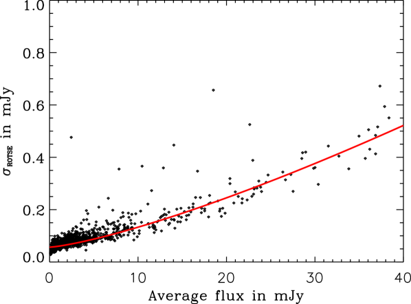
The estimated statistical error is crucial for simulating the detector noise behaviour, and therefore we have carried out a careful analysis of the detector noise as a function of the observed brightness. For the ROTSE-III data, we have estimated the total (statistical and systematic error) from the data: based upon $660$ individual pointings on PKS 2155-304, we have selected $\approx 3\,000$ other objects that are covered in these pointings. For each of these $3\,000$ light curves, the square root of the variance $\sigma_{\mathrm{ROTSE}}$ has been calculated. The correlation between $\sigma_{ROTSE}$ and the flux $\Phi$ of an object follows a power-law shape which has been parametrised with

$$\frac{\sigma_{\mathrm{ROTSE}}(\Phi)}{\mathrm{mJy}} = 0.0764\left(\frac{\Phi}{10\,\mathrm{mJy}}\right)^{1.302}+0.0564.$$ (1)

In order to neglect any variable objects median values have been used to perform a least-squares fit. The median values are calculated from the values within bins of $1$ mJy. The values and the fitted power-law are shown in Fig.1

Figure 1: Standard deviations $\sigma_{\mathrm{ROTSE}}$ of the light curves of $\approx 3\,000$ individual objects represented by the data points. The red curve is the least-squares fit to the medians of the values within $1$ mJy bins.

For the ASAS data, the quoted photometric uncertainty has been parametrised as a function of the total flux:

$$\frac{\sigma_{\mathrm{ASAS}}(\Phi)}{\mathrm{mJy}} = 0.162\left(\frac{\Phi}{10\,\mathrm{mJy}}\right)^{1.128}.$$ (2)

The photometric uncertainty on the archival plate data has been quoted to be in the range of $0.01\ldots 0.1$ magnitudes. These values are used to simulate the absolute uncertainties for the corresponding simulated data points.

3 Time series analysis

Two well-established methods – the Lomb-Scargle Periodogram (LSP) (see Appendix A.1) and the Structure Function (SF) (see Appendix A.2) – as well as a newly developed method called Multiple Fragments Variance Function (MFVF) (see Section 3.1) are used to characterise the timing behaviour of the optical long-term light curve of PKS 2155-304.

3.1 Multiple Fragments Variance Function (MFVF)

Figure 2: Flowchart of the Multiple Fragments Variance Function (MFVF).

We have developed an alternative method to characterise the variability of the source at different timescales in a simple and robust way. The variance

$$\mathrm{var}(a) := \langle(\langle a\rangle-a)^{2}\rangle$$ (3)

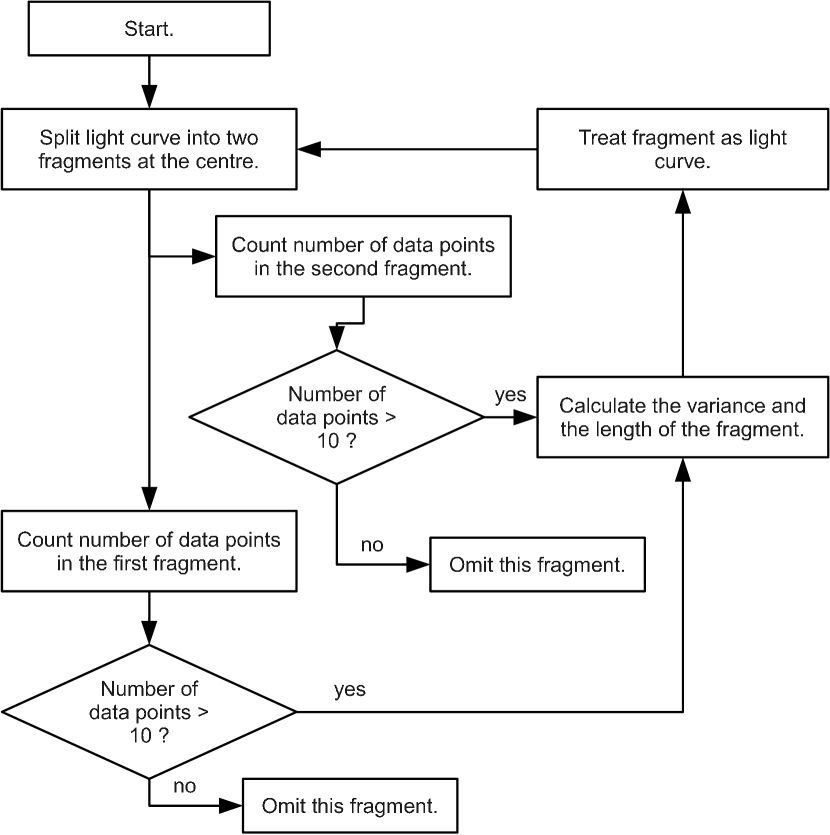
of the entire light curve is computed and subsequently, the light curve is subdivided at the half of the time lengths of the interval into two fragments and the variance for each of the two independent fragments is computed. This process of subdividing the light curve continues recursively until the number of remaining measurements within the fragment drops below a critical value (see Fig. 2 for a flowchart of this process). For the analysis carried out here, the requirement on the minimum number of measurements within the fragment is chosen to be $>10$. This number is a compromise between the limited number of measurements and the smallest timescale resolvable.

The fragment length is calculated by the time difference between the first and last measurement available within this fragment. The variance is therefore calculated for light curve segments which cover intervals with widely different values of duration. Finally, these values are averaged (binned) within 100 bins per decade of fragment length. This function yields information about the variance of the variability depending on the time scale.

Like the SF the MFVF is computed in the time domain. Unlike the other methods it is not sensitive to periodicities. It rather concentrates on information about the mean variability amplitude of the light curve occurring on a specific time scale. Therefore it is a goal-oriented method to find a maximum time scale of the variability. The sampling of the light curve is taken directly into account, so the distorting effect of uneven sampling is limited to an acceptable level (see below). An IDL as well as a Python script for the MFVF can be found at https://sourceforge.net/projects/mfvf/.

3.2 Comparison of the methods with simulated light curves

Since all methods suffer at various degrees from the effect of unevenly sampled light-curves (sampling effects), we use sets of simulated light-curves, in order to take sampling effects and the influence of instrumental noise into account. These simulated light-curves are useful to compare the behaviour of the three methods.

The simulated light curves are generated under the assumption of a red noise with a power spectral density function (PSD) following a power-law ($\mathcal{PSD}\propto f^{-\beta}$ above a characteristic frequency $f_{\mathrm{min}}$). The original recipe for generating pure red-noise light-curves first introduced by Timmer & Koenig (1995) has been extended to include a break at $f_{\mathrm{min}}$. For frequencies below $f_{\mathrm{min}}$, we assume a white noise behaviour ($\mathcal{PSD}=const.$). The normalisation of the simulated light curve is chosen to match the mean flux level and the variance of the measured light curve.
In order to investigate sampling effects the light curves were generated either with an even sampling (ideal case) or with an uneven sampling (realistic case). For both cases the total length $\Delta t_{\mathrm{total}}$ of the light curve and the number of data points $N_{\mathrm{obs}}$ are chosen to match the values of the light curve of PKS 2155-304. For the ideal case the observation times are spread evenly over $\Delta t_{\mathrm{total}}$. This results in an evenly sampled light curve with one measurement every $\Delta t_{\mathrm{total}}/N_{\mathrm{obs}}=3.37$ days and without any gaps.

For the realistic case the sampling is chosen to be exactly the same as it is for the light curve of PKS 2155-304. The raw evenly sampled simulated light curves are sampled down to the actual measurement times. Only for the realistic case each individual flux measurement has been randomised with a Gaussian function in order to account for experimental uncertainties on the measurements (see Section 2.3 for details on these uncertainties). For each data point the variance of the Gaussian errors were chosen individually to simulate the according instrumental noise.

For each case (ideal and realistic), 5 000 independent light curves (covering $\approx 27\,000$ days each) have been simulated with $\beta=2.0$ and $f_{\mathrm{min}}=10^{-3}$ d^-1. For the ideal case, all methods should produce results which are close to the intrinsic behaviour of the light curve. Here, the sampling effects are limited to the periodic sampling and to the finite length of the simulated light curves. By comparing the results from the realistic and ideal case simulations, sampling effects related to the uneven sampling can be investigated.

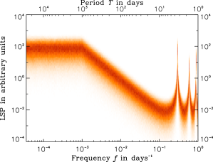
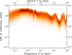
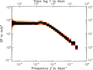
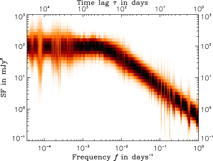
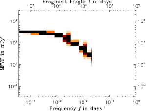
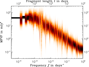
The individual values of the methods are accumulated in two-dimensional histograms. In Fig. 3, the histograms for the LSP (upper panel), SF (middle panel), and MFVF (lower panel) for the ideal case (left side) and the corresponding histograms for the realistic case (right side) are displayed. The resulting probability-density function (PDF) for a fixed value of frequency is shown in logarithmic bins ($10$ per decade).

The ideal case LSP (Fig. 3, upper panel left side) reproduces the simulated shape of a broken power-law with a visible deviation at high frequencies ($>0.1$ days^-1) related to the sampling frequency of $0.297$ days^-1. The LSPs from the uneven sampled light curves (right side) show a considerable flattening deviating from the original red noise behaviour. Additionally, the position of the break is smeared out over roughly half a decade in frequency. The flat (white) noise behaviour is distorted as well, showing a decrease of the LSP for decreasing frequencies. Besides the broad band distortion of the LSP, features in narrow frequency bands appear as a consequence of the sampling effects. Most notably is the drop in the LSP at a frequency of $1$ year^-1 due to the quasi-periodic sampling. The ideal case SF (Fig. 3, middle panel, left side) follows the expected behaviour for red noise $\mathcal{SF}\propto\tau^{\alpha}$ with $\alpha\approx\beta-1$ (Hughes et al. 1992; Lainela & Valtaoja 1993). For values of $\tau\gtrsim 0.3f_{\mathrm{min}}^{-1}$ the SF flattens out indicating the break in the simulated power-law. The break in the SF is smeared out into a gradual roll-over. The realistic case does not deviate systematically from the ideal case.

Finally, the result of analysing the light curve using the MFVF shows a consistent behaviour between the ideal and realistic simulations. In both cases, the simulated break at $f_{\mathrm{min}}^{-1}=1\,000$ d translates into a bend in the slope of the MFVF at a fragment length of $\approx 1\,000$ d. However for the ideal case no fragments shorter than $\approx 40\,\textrm{d}$ are found where the number of observations is greater than $10$ due to the even sampling. Therefore the MFVF is not defined at those time scales.

3.3 Best-fit estimates for $f_{\mathrm{min}}$ and $\beta$

Given that the sampling of the light-curve is generally not even, the results of the methods described above suffer from sampling and instrumental effects. Therefore, it is necessary to apply a forward folding technique to reliably reconstruct $f_{\mathrm{min}}$ and $\beta$. We have simulated $5\,000$ realistic light curves (as described in Section 3.2) for each parameter set on a grid of values of $0.8\leq\beta\leq 7.2$ in steps of $\Delta\beta=0.2$ and $-4.8\leq\log_{10}(f_{\mathrm{min}}/\mathrm{d}^{-1})\leq-2.2$ increasing in steps of $0.2$. For each set of parameters we have generated the PDFs for the LSP, SF and MFVF as described in Section 3.2. For the measured light curve a likelihood-estimator

$$\mathcal{L}(\beta,f_{\mathrm{min}}) = \sum\limits_{i=1}^{N}\log p_{i}(\beta,f_{\mathrm{min}}),$$ (4)

is calculated with $p_{i}(\beta,f_{\mathrm{min}})$ representing the probability to measure a value of e.g. the $\mathcal{LSP}(f_{i})$ for a given set of parameters $\beta$, $f_{\mathrm{min}}$ in the $i$-th bin. $p_{i}(\beta,f_{\mathrm{min}})$ is looked-up directly in the corresponding $\mathrm{PDF}(\beta,f_{\mathrm{min}})$. The best-fit $\mathrm{PDF}(\beta,f_{\mathrm{min}})$ maximises $\mathcal{L}(\beta,f_{\mathrm{min}})$ and determines the best-fit parameter set. It is noteworthy that the PDFs are not necessarily symmetric which requires the use of a likelihood instead of a least-squares function (Emmanoulopoulos et al. 2010). However, given that the individual probabilities are not independent of each other, the likelihood function is not well-defined. Nevertheless, the parameters which maximise the likelihood are good estimators for the best-fit parameters. It is not straightforward to estimate the uncertainties on the best-fit parameters given that the shape of the likelihood function (but not the position of its maximum) are considerably modified by the correlations between the individual probabilities (see also Section 4.3 on tests of the method and estimates for the uncertainties of the parameters). Since all simulated light curves are normalised to the same mean flux level and variance of the measured light curve, the methods are not sensitive to these parameters.

Figure 3: Two dimensional histograms of LSP, SF, and MFVF (from top to bottom) values of artificial light curves with $\beta=2.0$ and $f_{\mathrm{min}}=10^{-3}$ d^-1. On the left side histograms are shown for the case of an even sampling of one measurement every 3.37 days while on the right side, the effects of a realistic (uneven) sampling and simulated instrumental noise are visible (see text for details).

4 Results

4.1 Long-term optical light curve of PKS 2155-304

Figure 4: Optical light curve (R-band) of PKS 2155-304 measured with ROTSE.

Figure 5: Optical long-term light curve (R-band) of the core region of PKS 2155-304. The light curve combines ROTSE observations as well as other archival data (solid black circles: ROTSE, open purple circles: All-Sky-Automated-System, red open squares: Osterman et al. (2007), green solid squares: Zhang & Xie (1996), blue solid circles: Griffiths et al. (1979), black open squares: Tommasi et al. (2001)).

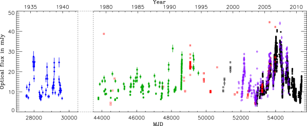
The optical R-band light curve measured with ROTSE is shown in Figure 4. The contribution of the host galaxy ($15.1^{\mathrm{mag}}$) is subtracted here and in the following. The gaps in the light curve are caused by bad weather periods or when PKS 2155-304’s position is too close to the sun. The light curve consists of $6\,310$ individual data points. The peak to peak amplitude observed during this time interval varies from $5$ to $40\,\textrm{mJy}$ indicating a relative variability of $35\,\textrm{mJy}$ or a factor for the flux of $\approx 8$. The variability amplitude is largest when comparing flux states separated by long time intervals (few years) while it decreases when comparing flux states on shorter timescales. This behaviour is typical of red noise.

In addition to the ROTSE-III measurements archival and contemporaneous data on PKS 2155-304, as described in Section 2, have been included in Fig. 5. Overall, the light curve covers the time from 1934 to 2010 with an extended gap between 1940 and 1979. Apparently, the maximum amplitude of variability in the long-term light curve is similar to the observed variability in the seven years of ROTSE-III observations. Before analysing the light curve in detail, this is a first indication that the red noise behaviour does not extend towards time scales much longer than a few decades.

4.2 Results of the time series analysis

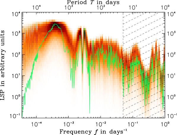
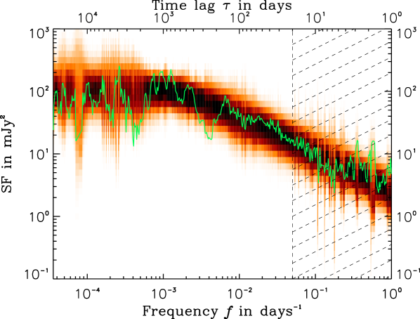
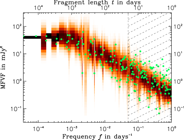
We have applied the three different methods described in Sections A.1, A.2, 3.1 to analyse the variability of the long-term light curve shown in Fig. 5. Based upon the resulting LSP, SF, and MFVF, the best-fit estimators for the power-law index $\beta$ as well as the break frequency $f_{\mathrm{min}}$ have been derived individually following a log-likelihood method described in Section 3.3

The instrumental noise for the archival data might be under- or overestimated. Therefore the variability on small time scales of a simulated light curve could be distorted to an unrealistic case. So we use only bins at time scales $>20$ days for the log-likelihood method to minimise systematic errors arising from this uncertainty.

The LSP of the long-term light curve of PKS 2155-304 is plotted in the top panel of Fig. 6 together with the PDF (histogram in colour scale) of the LSPs of the simulated light curves with the best-fitting parameters. The shape of the measured LSPs is in good agreement with the PDFs derived from simulations. As expected, sampling effects lead to a considerable distortion of the intrinsic power-law shape. Additionally, the uneven sampling produces features in the LSP which again are reproduced in the simulated data-sets.

In a similar fashion, the SF (middle panel in Fig. 6) as well as the MFVF (bottom panel in Fig. 6) are shown together with the PDF for the best fit. For both cases, the simulated and measured data-sets agree well with each other. Both, broad band shape and narrowband features from sampling effects are well reproduced in the simulated data.

For all methods, the resulting best-fit parameters for $\beta$ and $f_{\mathrm{min}}$ with their $1\sigma$ uncertainties are listed in Table 3. The uncertainties for the parameters are estimated as described in Section 4.3. Graphs with the log-likelihood functions for the parameters can be found in Appendix B.

Figure 6: Normalised Lomb Scargle Periodogram (LSP), Structure Function (SF) and Multiple Fragments Variance Function (MFVF) (from top to bottom). The green lines/points are the measured results of the light curve of PKS 2155-304. The histograms in colour scale represent the PDFs obtained from simulated light curves with the best-fit parameter sets $(\beta=5.0,\,f_{\mathrm{min}}=10^{-3.2}$ d${}^{-1})$, $(\beta=1.6,\,f_{\mathrm{min}}=10^{-3.4}$ d${}^{-1})$ and $(\beta=1.8,\,f_{\mathrm{min}}=10^{-3.0}$ d${}^{-1})$ respectively. Only the bins at $f<0.05\,\mathrm{d}^{-1}$ are used for the maximum-likelihood method.

Table 3: Best-fit parameters estimated by the methods separately.

Method	$\beta$	$\log(f_{\mathrm{min}}/\mathrm{d}^{-1})$
LSP	${5.0}^{+1.7}_{-3.0}$	${-3.2}^{+0.1}_{-0.4}$
SF	${1.6}^{+0.4}_{-0.2}$	${-3.4}^{+0.4}_{-0.5}$
MFVF	${1.8}^{+0.1}_{-0.2}$	${-3.0}^{+0.3}_{-0.4}$

4.3 Reliability of the method and estimates of the uncertainties

The likelihood method introduced above suffers from complex correlations between individual probabilities. This in turn requires to confirm that the method of maximising the likelihood estimator does actually provide a meaningful estimator of the underlying true parameters. Furthermore, it is necessary to estimate the statistical uncertainties on the best-fit parameters without relying on the usual method of calculating the second derivatives of the likelihood in the maximum.
Therefore an empiric approach is indicated. We have tested the reliability of the likelihood estimation with simulated light curves created with certain (well known) parameter sets. Again, 5 000 realistic light curves (as described in Section 3.2) have been simulated with the best-fit parameter set which has been found with the respective method. The light curves are analysed with the same methods as applied to the real light curve resulting in a distribution of best-fit parameter sets. The resulting distributions are then used to verify that the simulated parameters are reconstructed reliably and the width of the distributions provide a robust estimate of the uncertainties on the parameters. In Fig. 7 the two-dimensional histograms are displayed as contours (from top to bottom LSP, SF, and MFVF). The cross marks the simulated (input) parameters and the error bars indicate the 1 $\sigma$ confidence region for each parameter of the marginalised distributions which are plotted along the axes.
For the SF and MFVF, the input parameters are well recovered with relatively small uncertainties (see Table 3) while for the LSP, the reconstructed values are spread out over a large interval of $\beta$ resulting in large errors. While $f_{\mathrm{min}}$ is in very good agreement with the results of the SF and the MFVF, $\beta$ differs noticeably. However, this is in accordance to the large uncertainties of $\beta$ for the LSP, which is obviously affected by sampling effects. The LSP’s uncertainties for $\beta$ in the direction for higher values is probably underestimated, because the border of the grid is too close to the maximum of the likelihood.

Figure 7: Distribution of maximum likelihood estimates of simulated light curves with parameters found for PKS 2155-304. The boundaries of the coloured areas are the contours which are quoted as fractions of the $5\,000$ simulated light curves in the legends. The sub plots show the marginalised distributions which are calculated to obtain the $1\,\sigma$ error bars.

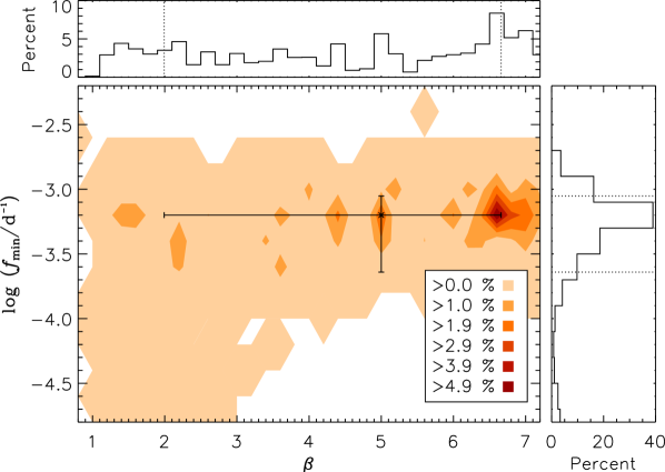
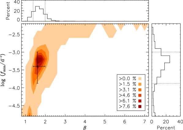
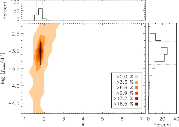
It remains to be demonstrated that the model and its best-fit parameters are a good characterisation of the data. Again, we use an approach relying on $5\,000$ simulated light curves to check the consistency of data and assumed model. As a goodness of fit estimate the value of $\mathcal{L}$ of the observed light curve is compared to the distribution of $\mathcal{L}$ of the light curves simulated with the best-fitting values of $\beta$ and $f_{\mathrm{min}}$. For the three different methods a fraction of $4\leavevmode\nobreak\$% (LSP), $3$ % (SF), and $50$ % (MFVF) of the simulated data are fit worse by the model than the actual data. Therefore the model is a reasonable description of the variability of the optical flux of PKS 2155-304.

5 Conclusion

We have presented an optical light-curve covering seven years of densely sampled (6 310 individual pointings) observations of PKS 2155-304 with the ROTSE-III telescopes in Namibia and Australia. Combined with archival data and ASAS observations, a long-term (sparsely sampled) light-curve going back to 1934 is analysed to characterise the red noise behaviour under the assumption that the power spectral density function (PSD) follows a power-law with slope $\beta$ and a break at a minimum frequency $f_{\mathrm{min}}$. At frequencies below $f_{\mathrm{min}}$, a white noise ($\beta=0$) PSD is assumed. For the analysis only time scales $>20$ days have been considered to avoid systematic errors due to uncertain estimates of the instrumental noise for the simulated light curves. The three different methods for analysing the long-term variability of PKS 2155-304 produce consistent results for simulated light curves with $\beta\approx 1.8$ and $f_{\mathrm{min}}\approx 1/1\,000\leavevmode\nobreak\$d^-1. The most precise result (discussed in the following) is given by the newly introduced Multiple Fragments Variance Function (MFVF), which is a straightforward method in the time domain to reveal information about the mean variability amplitude depending on different time scales. The result obtained with the first-order Structure Function (SF) is in very good agreement with the result of the MFVF. The slope of the Lomb-Scargle Periodogram (LSP) is affected strongly by sampling effects, so the uncertainties of the best-fit parameter $\beta$ are considerably larger for this method than for the MFVF and SF.

The power-law index of the PSD $\beta=1.8^{+0.1}_{-0.2}$ is harder than the value obtained by Paltani et al. (1997) at timescales smaller than 10 d ($\beta=2.4^{+0.3}_{-0.2}$). This may be an indication for an additional break or curvature in the PSD on short timescales. The power-law index of the red noise observed at other energy scales are similar. This hints at a common origin of the observed emission at the base of the jet.

Our analysis confirms the presence of red noise up to timescales of a few years without significant indications for any additional features as e.g. quasi-periodic oscillations. The existence of a break in the PSD at $f_{\mathrm{min}}=1/1\,000\,\mathrm{d}^{-1}$ is found to be significant at the level of $\approx 6\leavevmode\nobreak\ \sigma$ judging from the error on $f_{\mathrm{min}}$ estimated for the MFVF method. This break corresponds to a time scale of $\tau_{\mathrm{max}}\approx 2.7^{+2.2}_{-1.6}\,\textrm{yrs}$ after which the red noise behaviour disappears. In the context of SOC this time scale is linked to the “memory” of the system. At time scales longer than $\tau_{\mathrm{max}}$ the properties of the emission process de-correlate from its past. Due to causal reasons, the spatial dimension of the emission region is constrained to be $r<c\tau_{\mathrm{max}}=0.84^{+0.69}_{-0.50}\leavevmode\nobreak\ \,$pc.

The observed red-noise from PKS 2155-304 extends over five orders of magnitude in the time domain and over twelve orders of magnitude in the photon energy with apparently similar power-law slope. This implies that there is probably a link connecting particle acceleration processes on spatial scales ranging from ${\cal O}(100\,\mathrm{AU})$ to ${\cal O}(1\,\mathrm{pc})$.

Appendix A Standard methods of time series analysis

A.1 Lomb-Scargle Periodogram (LSP)

The normalised LSP (Lomb 1976; Scargle 1982) is a method to estimate the true underlying PSD of the variability of unevenly sampled time series data. For a given set of values $a_{i}:=a(t_{i})$ measured at the times $t_{i}$ the LSP is defined as

$$\mathcal{LSP}(\omega)=\frac{1}{2\sigma^{2}}\left\{\frac{\left[\sum_{j}\left(a_{j}-\bar{a}\right)\,\cos\left(\omega\left(t_{j}-\epsilon\right)\right)\right]^{2}}{\sum_{j}\cos^{2}\left(\omega\left(t_{j}-\epsilon\right)\right)}\right.$$

$$+\left.\frac{\left[\sum_{j}\left(a_{j}-\bar{a}\right)\,\sin\left(\omega\left(t_{j}-\epsilon\right)\right)\right]^{2}}{\sum_{j}\sin^{2}\left(\omega\left(t_{j}-\epsilon\right)\right)}\right\},$$ (5)

with $\omega=2\pi f$, $\sigma^{2}$ being the variance and $\bar{a}$ the mean value of the time-series $a_{i}$. The time delay

$$\epsilon = \frac{1}{2\omega}\tan^{-1}\frac{\sum_{j}\sin\left(2\omega t_{j}\right)}{\sum_{j}\cos\left(2\omega t_{j}\right)}$$ (6)

is required to achieve that $\mathcal{LSP}(\omega)$ is invariant under a change of the phase (Press & Rybicki 1989). In order to weigh widely different frequency scales equally, we calculate the LSP for values of $f$ with a constant interval of 0.01 decades on a logarithmic scale.

A.2 Structure Function (SF)

The first order SF (Simonetti et al. 1985) for a time-lag $\tau$ between any pair of observations is defined as

$$\mathcal{SF}(\tau)=\frac{1}{n}\sum_{t_{i}}\left[a\left(t_{i}+\tau\right)-a\left(t_{i}\right)\right]^{2},$$ (7)

with $n$ being the number of summands. The structure function can only be computed for discrete values of $\tau$ that exist in the time series:

$$\tau\in\left\{\left|t_{i}-t_{j}\right|:t_{i},t_{j}\in T\right\}\;,$$ (8)

where $T$ is the set of times where measurements have been carried out. Commonly, the values of the structure function are combined and averaged in intervals of $\tau$ to smooth fluctuations on time scales shorter than the width of the bins. In order to weigh widely different time scales equally, we choose a constant bin width of $0.01$ decades on a logarithmic scale.

Appendix B Log likelihood

Figure 8: Logarithm of the likelihood for the real light curve being realised by red noise with a certain $\beta$ and $f_{\mathrm{min}}$. Top for the LSP, middle for the SF and bottom for the MFVF. The peaks located in the white shaded areas are marked with a black cross.

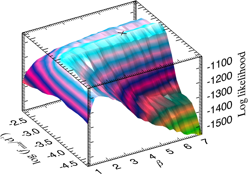
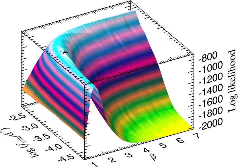
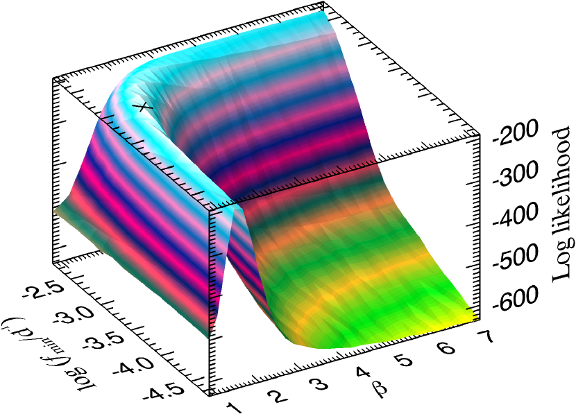
The log-likelihood values for the grid of the parameters are shown in the panels (from top to bottom LSP, SF, and MFVF) of Fig. 8. The log-likelihood functions $\mathcal{L}$ of the SF and MFVF have a similar shape with a ridge-like region with a bend. For the SF and the MFVF the maximum is located in the region where the ridge bends. For the LSP, the maximum of the likelihood is located on a ridge which is oriented along the direction of increasing $\beta$, which obviously does not constrain the best-fit value of $\beta$ very well.