Characterizing exoplanetary atmospheres through infrared polarimetry

Abstract

Planets can emit polarized thermal radiation, just like brown dwarfs. We present calculated thermal polarization signals from hot exoplanets, using an advanced radiative transfer code that fully includes all orders of scattering by gaseous molecules and cloud particles. The code spatially resolves the disk of the planet, allowing simulations for horizontally inhomogeneous planets. Our results show that the degree of linear polarization, $P$, of an exoplanet’s thermal radiation is expected to be highest near the planet’s limb and that this $P$ depends on the temperature and its gradient, the scattering properties and the distribution of the cloud particles. Integrated over the disk of a spherically symmetric planet, $P$ of the thermal radiation equals zero. However, for planets that appear spherically asymmetric, e.g. due to flattening, cloud bands or spots in their atmosphere, differences in their day and night sides, and/or obscuring rings, $P$ is often larger than 0.1%, in favorable cases even reaching several percent at near-infrared wavelengths. Detection of thermal polarization signals can give access to planetary parameters that are otherwise hard to obtain: it immediately confirms the presence of clouds, and $P$ can then constrain atmospheric inhomogeneities and the flattening due to the planet’s rotation rate. For zonally symmetric planets, the angle of polarization will yield the components of the planet’s spin axis normal to the line-of-sight. Finally, our simulations show that $P$ is generally more sensitive to variability in a cloudy planet’s atmosphere than the thermal flux is, and could hence better reveal certain dynamical processes.

1 Introduction

Studying the thermal emission of exoplanets has only recently become possible with the direct detections of young giant planets in wide orbits around their star (e.g. Marois et al., 2008; Lafrenière et al., 2008) and secondary eclipse detections of transiting exoplanets in tight orbits (see Deming & Seager, 2009). These hot planets emit most of their radiation at near-infrared wavelengths and flux measurements at different wavelengths are used to constrain properties of their atmospheres. However, little attention has been given to the information contained within the polarization signals of this planetary thermal radiation.

Incident starlight will usually get polarized when it is scattered by gases and particles in a planetary atmosphere. When integrated over the planetary disk, the reflected starlight can yield a significant net degree of polarization (e.g. Seager et al., 2000; Stam et al., 2004). Also polarization in stellar atmospheres is well-known (e.g. Harrington, 1970) and a dozen polarized brown dwarfs have been identified (e.g. Ménard et al., 2002). Thermal radiation that is emitted by a body can get polarized upon scattering. For a net polarized thermal signal of a spatially unresolved body such as a brown dwarf or an exoplanet to be observable, not only scattering particles are required, but also an asymmetry in the body’s disk. Otherwise, the polarized thermal signals from different parts of the disk will cancel each other completely. With an asymmetric disk, the cancellation will be incomplete and a net polarization signal remains.

For the polarized brown dwarfs, a plausible source of asymmetry is the flattening of the body due to its rotation, as advocated by Sengupta & Marley (2010). Very recently, these authors have extended their work on polarization of flattened objects to planets as well (Marley & Sengupta, 2011). In a planetary atmosphere, sources of asymmetry could arise from horizontal inhomogeneities in temperature or cloud thickness. For instance, strong zonal winds can cause banded structures, as found on all giant planets in our solar system. Furthermore, rings that obscure or shadow part of the planetary disk would cause asymmetries.

Here, we will use simulated signals of horizontally inhomogeneous planets to present processes that polarize thermal planetary radiation, to explore parameters that determine the strength of these thermal polarization signals, and to discuss the value of infrared polarimetry for the characterization of exoplanet atmospheres.

2 Our numerical model

Light is fully described by a flux vector ${\bf F}=(F,Q,U,V)$, with $F$ the total flux, $Q$ and $U$ the linearly polarized fluxes, and $V$ the circularly polarized flux (Hansen & Travis, 1974). Parameters $Q$ and $U$ are defined with respect to a given reference plane. For atmospheric calculations we have a local reference plane with axes parallel and normal to the local planetary horizon. In the following, we will neglect $V$, and express the degree of polarization, $P$, using

$$P=\frac{\sqrt{Q^{2}+U^{2}}}{F}$$ (1)

The angle of polarization, $\chi$, with respect to the reference plane is defined as (see Hansen & Travis, 1974)

$$\tan 2\chi=U/Q.$$ (2)

We calculate the radiative transfer in a locally plane-parallel, vertically inhomogeneous planetary atmosphere for a range of emission angles using a doubling-adding method (Wauben et al., 1994), which fully includes all orders of scattering and polarization. Each atmosphere consists of 40 layers, equally spaced in log pressure, with pressures $p$ between 10^-6 bar (top) and 5 bar (bottom). In order to make comparisons between different model atmospheres we use ad hoc temperature profiles, assuming hydrostatic equilibrium, which are uniform in temperature $T$ for $p<10^{-3}$ bar and $p>1$ bar. In between these pressures the near-infrared emission originates and we assume $dT/d\ln{p}$ is constant there, pivoting around $T=1500$ K at $p=33$ mbar for different temperature profiles. We perform our calculations at $\lambda_{1}=1.05$ $\mu$m, which is in the continuum ($Y$-band), and at $\lambda_{2}=1.11$ $\mu$m, in a water vapor absorption band. The water absorption optical depths are calculated using the HITEMP 2010 database (Rothman et al., 2010), assuming Voigt line shapes and a volume mixing ratio of 5$\cdot$10^-4.

At these infrared wavelengths, the scattering optical thickness of the gas molecules is negligible, but radiation can be scattered by larger cloud/dust particles. We calculate the scattering matrices of the particles in our model atmospheres using Mie-scattering as described by de Rooij & van der Stap (1984) (thus assuming spherical particles). The particles that we use are small compared to the wavelength and have unity single scattering albedo. The scattering of these particles can be described as Rayleigh-scattering, with a nearly isotropic flux phase function and a bell-shaped polarization phase function reaching almost 100% polarization at a single scattering angle of 90^∘. The particles are assumed to be in one of the atmospheric layers and we assume identical cloud optical thicknesses at $\lambda_{1}$ and $\lambda_{2}$, which only have a difference in wavelength of 0.05 $\mu$m. We also performed calculations using larger, non-Rayleigh-like, particles, which will be discussed in Section 3.4.

3 Spatially resolved polarimetry

To understand disk-integrated polarization signals of exoplanets better, we first discuss polarization signals that are spatially resolved across the disk.

Generally, singly scattered radiation is unpolarized for scattering angles equal or close to 0^∘ (assuming unpolarized incoming radiation, Hansen & Travis, 1974). Hence, thermal radiation emitted by low atmospheric layers that is scattered upward by particles in upper layers will have a very low degree of polarization. Radiation that is emitted in a high altitude layer that itself contains scattering particles can also be scattered in the upward direction over a 90^∘ angle and be strongly polarized, in particular when the scattering is Rayleigh-like. However, because the scattering particles in the upper layer will receive emitted radiation from all directions equally, the net polarization of the scattered radiation that emerges from the layer will equal zero. Hence, at the center of a horizontally homogeneous planetary disk, $P$ will usually be low, regardless of the temperature profile.

At the limb of a planetary disk, thermal radiation that is emitted by low atmospheric layers will be scattered by particles in upper layers towards the observer over angles near 90^∘, yielding high values of $P$. Radiation that is emitted in high altitude layers that contain scattering particles themselves will yield relatively low values of $P$, because of the large range of scattering angles. $P$ will not be zero mainly because of contributions of radiation that has been scattered twice or more.

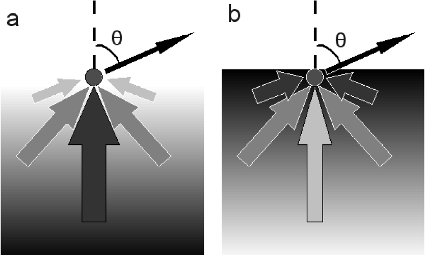
Figure 1: Sketch of thermal radiation with emission angle $\theta$, that is scattered by a particle high in the planetary atmosphere, with dark areas indicating higher temperatures and thus larger thermal fluxes. Panel (a) illustrates a positive temperature gradient, and panel (b) a negative one.

The degree of polarization at the limb thus depends strongly on the temperature structure of the atmosphere. This is related to the limb darkening effect, which is illustrated in Figure 1. For a given optical path length, radiation arriving at an angle towards the scatterer will come from a higher layer in the atmosphere than the light coming from directly below. If there is a temperature gradient, that difference in altitude will correspond to a difference in temperature and hence a difference in thermal flux. If the temperature decreases with decreasing pressure, most thermal radiation emerging from the limb of the planet will have been emitted in the lower atmospheric layers, and will have been scattered at high altitudes towards the observer at angles close to 90^∘, where $P$ of Rayleigh scattered radiation is highest. If the temperature increases with decreasing pressure, most of the thermal radiation that is observed at the planet’s limb will have been emitted and scattered in the upper layers. In this case, the large range of scattering angles will yield relatively low values of $P$ (see Figure 1). If the temperature gradient equals zero, the radiation field around the scatterers is more symmetric, even at the limb, and the net $P$ of radiation emitted towards the observer will be close to zero.

3.1 Dependence on temperature gradient

Figure 2a shows the normalized polarized flux $-Q/F$ for model atmospheres with different temperature profiles and a high altitude cloud layer with an optical thickness of 0.1 at $\lambda_{1}$ and $\lambda_{2}$ for small and large emission angles. In these one-dimensional model calculations, $U=0$, and hence $|Q/F|=P$. A positive (negative) $-Q/F$ indicates that the radiation is polarized parallel (perpendicularly) with respect to the local horizon. The curves in Figure 2a show the strong influence of the temperature gradient on $P$ and that a positive temperature gradient changes the polarization angle $\chi$ by 90^∘.

It is also clear that for positive temperature gradients, $P$ is highest for $\lambda_{2}$, the wavelength in the water vapor absorption band. This can again be understood in terms of the effect shown in Figure 1. In the continuum, the radiation that arrives at the scattering particle originates deeper in the atmosphere than in the water band. Because of our constant temperature gradient, the temperature difference between radiation coming towards the particle from directly below and that coming at an angle will be roughly similar for both wavelengths. However, such a temperature difference corresponds to a relatively larger difference in flux for lower temperatures, meaning that radiation arriving from the colder atmospheric layers probed in the absorption band will have relatively more contributions from directly below and hence will give a larger $P$ at the limb. For negative temperature gradients, $-Q/F$ is negative, which shows that here the emerging signal is dominated by radiation arriving at an angle (see Figure 1b) that is scattered multiple times. In the continuum, there is now relatively less radiation arriving from directly below, giving less positive contributions to the net $-Q/F$ value. Hence, $P$ is higher in the continuum than in the absorption band for atmospheres with a negative temparature gradient and high clouds.

3.2 Dependence on cloud optical thickness

An optically very thin cloud won’t affect the outgoing radiation much as the cloud is almost transparent to the outward-going radiation. Hence, not much radiation is scattered and $P$ will be low. With increasing cloud optical thickness, $P$ will increase, because more radiation is scattered as the transmission of the clouds decreases. On the other hand, the contribution of multiple scattered radiation will also increase with increasing cloud (scattering) optical thickness. This is because the free path length of the radiation can become less than the distance between scattering particles. Multiple scattered radiation arriving at the observer will have been scattered at a range of angles. At the limb, this means that the observed radiation has not only been scattered over angles that produce a high $P$, but it will also have been scattered over angles that produce low $P$. For small emission angles, such as observed near the center of the planetary disk, multiple scattering can actually increase $P$, because it adds radiation that has been scattered at angles where $P$ is large. For very large optical thicknesses, virtually all the thermal radiation will originate from the cloud and be multiple scattered within the cloud itself and $P$ will be relatively low. These various effects of the cloud optical thickness can be seen in Figure 2b: first $P$ increases with cloud optical thickness as more radiation is scattered, then $P$ decreases as multiple scattering becomes important, and finally $P$ stays roughly constant at large cloud optical thicknesses as virtually all radiation originates from multiple scattering within the cloud itself.

3.3 Dependence on cloud top height

In Figure 2, the cloud is located high in the atmosphere. Lowering the cloud does not change $P$ much until the gas absorption optical depth is comparable to the cloud scattering optical thickness. For optically thin clouds, $P$ gradually vanishes as the cloud descents and gaseous absorption starts dominating over scattering. For thicker clouds, $P$ at the limb will first rise slightly before vanishing as multiple scattering effects are reduced. Because gas optical thicknesses depend on wavelength, cloud top heights can have large effects on $P$’s spectral behavior. For instance, in gaseous absorption bands, $P$ can be zero when clouds are below the altitudes where gaseous absorption is high, whereas it can be non-zero at continuum wavelengths. Hence, a case with low clouds can leave peaks in the polarization spectrum at certain wavelengths, whereas in a case with high clouds these wavelengths represent a local minimum in the polarization spectrum.

3.4 Dependence on scattering properties

In the previous calculations, we assumed particles that were small relative to the wavelength (i.e. they are Rayleigh scattering). The polarization signal of a planet will, however, depend on the particles’ scattering properties. With increasing particle size, the maximum value of the polarization phase functions usually decreases and polarization direction changes occur (e.g. Stam et al., 2004). Calculations with Saturn-like particles, whose scattering properties are derived by Tomasko & Doose (1984), and 1-$\mu$m spherical Mg₂SiO₄ particles show that $P$ at the limb will decrease to less than 10% and that the sign of $Q$ will be opposite to that shown in Figure 2. In both of these cases the single scattering albedo of the particles is close to unity.

3.5 Three-dimensional effects

The above calculations were performed using one-dimensional models, which are applicable to atmospheres that are locally horizontally homogeneous. However, large local variations in e.g. temperature or composition can give rise to adjacency effects that affect a planet’s polarization signal. For instance, a hot spot in an atmosphere could be surrounded by a ring of high polarization resulting from radiation that is emitted by the hot spot, which is subsequently scattered by the colder atmosphere around it. Such three-dimensional effects can be the subject for later study.

4 Disk-integrated polarimetry

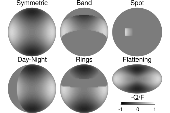
Figure 3: Simulated images of normalized $-Q/F$ across the planetary disk for the model planets presented in this paper. Integrating $-Q/F$ over the disk yields $P=0$ for the spherically symmetric planet, while it will usually leave a net $P$ for the other cases.

To simulate exoplanet signals, we integrate the spatially resolved fluxes across the planetary disk, using a grid with a 2^∘ resolution in latitude and longitude. The reference plane for the polarized fluxes $Q$ and $U$ depends on the location on the planet (Wauben et al., 1994). Before integrating these fluxes, we thus have to rotate the local flux vectors to the planet’s global reference plane (Hovenier & van der Mee, 1983; Stam et al., 2006), which we align with the planet’s spin axis. For spherically symmetric planets, the rotation and subsequent integration yields a complete cancellation of both $Q$ and $U$ of the planetary thermal radiation (see Figure 3).

We have performed calculations for five different asymmetric planets, all illustrated in Figure 3: spherical planets with a band, a spot, obscuring rings (without ring shadows), a day-night difference, and a flattened (ellipsoidal) planet with a horizontally homogeneous atmosphere. Obviously, the parameter space for these calculations is enormous. Here, we present a limited number of cases to provide an indication of the range of polarization signals of inhomogeneous planets and to draw some qualitative conclusions. We model our horizontally inhomogeneous planets using two different atmospheric profiles, and hence two different one-dimensional radiative transfer calculations (at several emission angles). Depending on the case (band, spot, etc.) and viewing geometry, we assign one of the two profiles to the grid points on the planet. We use a temperature gradient of 300 K/$\ln{p}$ everywhere on the planet, but in the clear parts of the planet, temperatures are 250 K lower than in the cloudy parts, which is a modest temperature contrast for hot Jupiters (Showman et al., 2009). In best-fit model calculations of the directly imaged planets around HR 8799 and 2M1207 by Barman et al. (2011b, a) the temperature gradient at pressure higher than 0.1 bar is on average steeper than the 300 K/$\ln{p}$ used here, whereas below this pressure the temperature gradient is more shallow. The temperature profile shown in Marley & Sengupta (2011) shows very similar behaviour for $T_{\mathrm{eff}}$=1000 K, $g$=30 m s^-2 and $f_{\mathrm{sed}}$=2, although temperature gradients are slightly less steep around 0.1 bar. Also best-fit atmospheres of transiting exoplanets have temperatures gradients around 300 K/$\ln{p}$ in the lower atmosphere (Madhusudhan & Seager, 2009; Madhusudhan et al., 2011b). In the near-infrared, most of the thermal emission originates from the region in the atmosphere between 0.1-1 bar for positive temperature gradients (e.g. Showman et al., 2009; Madhusudhan et al., 2011b), and hence our assumed temperature gradient does not seem unreasonably steep. For the cloudy part of the atmosphere, a Rayleigh scattering cloud layer with unity scattering optical thickness is placed at the top of the atmosphere.

Our calculations of ellipsoidal planets can be compared to those by Sengupta & Marley (2010). For a homogeneous cloudy atmosphere and an inclination angle of 90^∘, our $P$ at $\lambda_{1}$ as a function of oblateness compares well with the $I$-band $P$ of Sengupta & Marley (2010) for e.g. $T_{\mathrm{eff}}=1800$ K with $\log(g)=4.5$ and $f_{\mathrm{sed}}$=2 (see their Figure 1). Like Sengupta & Marley (2010), we can reach values of $P$ of several percent for extreme oblatenesses at $\lambda_{1}$, and roughly twice that value at $\lambda_{2}$. Longer wavelengths will give only slightly lower $P$s, given identical temperatures and optical depths, as is shown in Fig. 4 (the cloud optical thickness is kept constant with wavelength). The figure also shows the effect of low clouds, which results in inverted polarization spectra. Also note the large difference in polarization spectra between the two cases, whereas the flux spectra are very similar. Calculations with 1-$\mu$m Mg₂SiO₄ particles, with a cloud optical thickness of unity at 1 $\mu$m and wavelength-variations over the plotted wavelength range determined by Mie theory, result in very similar polarization spectra, scaled down by a factor of $\sim$5.

For the planet with the equatorial cloud band, we varied the band’s latitudinal width and the planet’s inclination angle. A clear planet with a dusty band shows a maximum $P$ (0.5% at $\lambda_{1}$ and 2% at $\lambda_{2}$) for a 40^∘-60^∘ wide band. For a given band width, $P$ decreases with decreasing inclination angle, to increase again slightly when inclination angles get larger and the band reaches the limb. When the planet is seen exactly pole-on, $P=0$ again, as expected. For a dusty planet with a clear band, $P$ can reach 0.5% at $\lambda_{1}$ and 4% at $\lambda_{2}$, depending on the inclination angle.

Except for very special geometries, rings will usually obscure part of a planet either directly or through shadowing. We simulated the presence of cold, optically thick rings for a range of inclination angles by modeling the obscured part of the disk with a 200 K blackbody (see Figure 3). For a ring-planet radius ratio similar to that of Saturn, $P$ is at most 0.3% at $\lambda_{1}$ and 0.8% at $\lambda_{2}$ at a ring inclination angle of $\sim$45^∘. If the rings extend further outwards, and hence cover a larger fraction of the planet’s disk, the maximum value of $P$ increases by a few tenths of a percent. Note that we only modelled the obscuration here. The rings themselves can scatter the thermal radiation from the planet and might also emit significant polarized radiation themselves if they are hot and optically thick. A three-dimensional model of the planet and rings would be needed to model the interplay between planet and rings.

All three cases above have the planet’s spin axis as the axis of symmetry. As a result, the disk-integrated polarized flux $U$ equals zero and the angle of polarization $\chi$ is either parallel or perpendicular to the spin axis, depending on the particles’ microphysical properties and the temperature profile. We now briefly discuss two cases without this type of symmetry.

We simulated an equatorial cloudy hot spot by a dusty square of $20^{\circ}\times 20^{\circ}$ (latitude $\times$ longitude) (see Figure 3). As the planet rotates, $F$ varies mildly, while $P$ and $\chi$ vary significantly (see Figure 4). Here, $P$ reaches 0.1% at $\lambda_{1}$, and 0.6% at $\lambda_{2}$.

The planet with the day-night difference has a dusty and a clear hemisphere (split along longitude lines, parallel to the terminator). As the planet rotates, $P$ depends on which parts of the hemispheres are in view. The maximum $P$ equals 0.6% at $\lambda_{1}$ and 4% at $\lambda_{2}$, and $P=0$ when only one hemisphere is in view. $\chi$ varies similarly to the spot case (Figure 4). Again, flux $F$ varies only mildy compared to $P$.

5 Conclusions and opportunities for exoplanet characterization

We have calculated polarization signals of thermal radiation that is scattered by particles in exoplanet atmospheres. Important parameters that determine the degree of linear polarization $P$ are the particles’ polarization phase function, the optical thickness and the altitude of the particles, and the temperature and its gradient.

For spatially resolved planets, $P$ is usually highest near the planet’s limb. For spatially unresolved planets, inhomogeneities on a planet’s disk can cause a net polarization signal. In the cases we have considered (i.e. a band, a spot, obscuring rings, a day-night difference and a horizontally homogeneous flattened disk), $P$ was typically above 0.1%, and values of several percent were reached in favorable cases. Combining different effects, e.g. a band on a flattened planet, could increase $P$ even further. With a high cloud and a positive temperature gradient, $P$ is higher in gaseous absorption bands than in the surrounding continuum. Unfortunately, little flux is emitted in those bands in this case. Together with telluric absorption, this will make the water absorption bands of planets with a positive temperature gradient less suitable for detection of infrared polarization in exoplanets using ground-based telescopes. Fortunately, $P$ is at most a factor of a few lower in the atmospheric windows, whereas the flux can be several magnitudes higher, giving more opportunities for detection there.

Currently, exoplanetary thermal radiation is detected either during secondary eclipses of transiting planets or through direct imaging of planets at large orbital distances. In the former case the combined light of the star and planet is measured, and although these usually tidally locked planets are expected to display large temperature inhomogoneities, measuring a 1% polarization signal of the planet will be very challenging, as sensitivities of $\sim$10^-6 need to be reached. Indeed, direct imaging, where the planet is spatially resolved from its star, promises to be a more suitable method to detect polarized exoplanets, especially with new instruments like Gemini/GPI and VLT/SPHERE.

There are several reasons why planets like those in the HR 8799 system might be more prone to producing polarized signals than brown dwarfs, which can be polarized by a few percent. Firstly, the surface gravity of planets is lower than that of brown dwarfs, making them more flattened for a given rotation rate (see also Marley & Sengupta, 2011). Secondly, broadband flux measurements suggest the HR 8799 planets to be more cloudy than most brown dwarfs, which might be a common feature of young planets (Madhusudhan et al., 2011a). Thirdly, the effective temperatures in the planets’ atmospheres are lower than those in known polarized brown dwarfs and, given a certain temperature gradient, lower temperatures will yield higher $P$.

A detection of an infrared polarized signal will immediately confirm the presence of scattering particles in the planetary atmosphere. In addition, the polarization angle $\chi$ will reveal the components of the planet’s spin axis normal to the line-of-sight for a zonally symmetric planet. For such planets, both $P$ and $F$ will show little variability. On the other hand, if the polarization is caused by moving clouds or hot spots, both $P$ and $\chi$ will vary in time, and stronger than $F$. Hence, a time series of $P$ and $\chi$ will give insight into the underlying source, and a periodic signal could even yield atmospheric rotation rates. However, some cases, like a banded and an oblate planet, may give very similar flux and polarization spectra and disentangling the two cases might be very difficult. Knowledge of the gravity on a planet will perhaps help in such a case, as the gravity is strongly connected to the possible oblateness.

Together with flux measurements, polarimetry can also constrain particle properties, like their scattering albedo and size. Using polarimetry, one could for instance distinguish between absorbing iron particles and scattering silicate particles, which yield similar fits to flux spectra (Madhusudhan et al., 2011a). Fig. 4 also shows that the polarization spectrum is much more sensitive to e.g. cloud top heights than the flux spectrum. Furthermore, the broadband polarization is sensitive to the atmospheric temperature gradient, which is not easily obtained from broadband flux measurements.

Figure 2: Normalized polarized fluxes $-Q/F$ at $\lambda=1.05\mu$m (solid lines) and 1.11 $\mu$m (dashed lines) for atmospheres with (a) different temperature gradients and a high altitude cloud with optical thickness 0.1, and (b) a temperature gradient of 300 $K/\ln{p}$ and different cloud optical thicknesses. Thick lines indicate emission angles of 80^∘ and thin lines those of 30^∘.

Figure 4: Normalized $F$ and $P$ as a function of wavelength for a homogeneous, flattened planet with oblateness of 0.3. Solid lines indicate models with clouds at the top of the atmosphere, dotted lines with clouds at 0.015 bar. $P$ is only plotted for $F>4\cdot 10^{-3}$ as small integration errors at these low flux levels give rise to very noisy $P$ spectra there.

Figure 5: Normalized $F$, $P$, and $\chi$ at $\lambda_{2}$ of a rotating planet with a 20^∘x20^∘ dusty hot spot on its equator. The longitude denotes the distance of the spot with respect to the sub-observer point.

References

- Barman et al. (2011a) Barman, T. S., Macintosh, B., Konopacky, Q. M., & Marois, C. 2011a, ApJ, 733, 65
- Barman et al. (2011b) Barman, T. S., Macintosh, B., Konopacky, Q. M., & Marois, C. 2011b, ApJ, 735, L39+
- de Rooij & van der Stap (1984) de Rooij, W. A. & van der Stap, C. C. A. H. 1984, A&A, 131, 237
- Deming & Seager (2009) Deming, D. & Seager, S. 2009, Nat, 462, 301
- Hansen & Travis (1974) Hansen, J. E. & Travis, L. D. 1974, Space Sci. Rev., 16, 527
- Harrington (1970) Harrington, J. P. 1970, Ap&SS, 8, 227
- Hovenier & van der Mee (1983) Hovenier, J. W. & van der Mee, C. V. M. 1983, A&A, 128, 1
- Lafrenière et al. (2008) Lafrenière, D., Jayawardhana, R., & van Kerkwijk, M. H. 2008, ApJ, 689, L153
- Madhusudhan et al. (2011a) Madhusudhan, N., Burrows, A., & Currie, T. 2011a, ArXiv e-prints
- Madhusudhan et al. (2011b) Madhusudhan, N., Harrington, J., Stevenson, K. B., et al. 2011b, Nature, 469, 64
- Madhusudhan & Seager (2009) Madhusudhan, N. & Seager, S. 2009, ApJ, 707, 24
- Marley & Sengupta (2011) Marley, M. S. & Sengupta, S. 2011, ArXiv e-prints
- Marois et al. (2008) Marois, C., Macintosh, B., Barman, T., et al. 2008, Science, 322, 1348
- Ménard et al. (2002) Ménard, F., Delfosse, X., & Monin, J. 2002, A&A, 396, L35
- Rothman et al. (2010) Rothman, L. S., Gordon, I. E., Barber, R. J., et al. 2010, J. Quant. Spectro. Rad. Trans., 111, 2139
- Seager et al. (2000) Seager, S., Whitney, B. A., & Sasselov, D. D. 2000, ApJ, 540, 504
- Sengupta & Marley (2010) Sengupta, S. & Marley, M. S. 2010, ApJ, 722, L142
- Showman et al. (2009) Showman, A. P., Fortney, J. J., Lian, Y., et al. 2009, ApJ, 699, 564
- Stam et al. (2006) Stam, D. M., de Rooij, W. A., Cornet, G., & Hovenier, J. W. 2006, A&A, 452, 669
- Stam et al. (2004) Stam, D. M., Hovenier, J. W., & Waters, L. B. F. M. 2004, A&A, 428, 663
- Tomasko & Doose (1984) Tomasko, M. G. & Doose, L. R. 1984, Icarus, 58, 1
- Wauben et al. (1994) Wauben, W. M. F., de Haan, J. F., & Hovenier, J. W. 1994, A&A, 282, 277