Non-Newtonian characteristics of peristaltic flow of blood in micro-vessels

Abstract

Of concern in the paper is a generalized theoretical study of the non-Newtonian characteristics of peristaltic flow of blood through micro-vessels, e.g. arterioles. The vessel is considered to be of variable cross-section and blood to be a Herschel-Bulkley type of fluid. The progressive wave front of the peristaltic flow is supposed sinusoidal/straight section dominated (SSD) (expansion/contraction type); Reynolds number is considered to be small with reference to blood flow in the micro-circulatory system. The equations that govern the non-Newtonian peristaltic flow of blood are considered to be non-linear. The objective of the study has been to examine the effect of amplitude ratio, mean pressure gradient, yield stress and the power law index on the velocity distribution, wall shear stress, streamline pattern and trapping. It is observed that the numerical estimates for the aforesaid quantities in the case of peristaltic transport of the blood in a channel are much different from those for flow in an axisymmetric vessel of circular cross-section. The study further shows that peristaltic pumping, flow velocity and wall shear stress are significantly altered due to the non-uniformity of the cross-sectional radius of blood vessels of the micro-circulatory system. Moreover, the magnitude of the amplitude ratio and the value of the fluid index are important parameters that affect the flow behaviour. Novel features of SSD wave propagation that affect the flow behaviour of blood have also been discussed.
Keywords: Non-Newtonian Fluid; Flow Reversal; Wall Shear Stress; Trapping; SSD Wave.

1 Introduction

Peristaltic transport of fluids through different vessels of human physiological systems is known to physiologists as a natural mechanism of pumping materials. The phenomenon of peristalsis has important applications [1, 2, 3, 4] in the design and construction of many useful devices of biomedical engineering and technology, artificial blood devices such as heart-lung machine, blood pump machine, dialysis machine etc. Apart from physiological studies, many of the essential fluid mechanical characteristics of peristalsis have also been elucidated in analyses of different engineering problems carried out by several researchers. These characteristics become more prominent when the flow is induced by progressive waves of area contraction/expansion along the length of the boundary of a fluid-filled distensible tube. Benefits that can be derived from studies on peristaltic movement have been elaborately discussed in our earlier communications [5, 6, 7, 8, 9, 10, 11, 12, 13, 14]. Further discussion on peristalsis was made by several other researchers (cf. Guyton and Hall [15], Jaffrin and Shapiro [16], Srivastava and Srivastava [31], Vajravelu et al. [18], Hayat et al. [19]).

Nomenclature
$R,\theta,Z$	Cylindrical co-ordinates
$c$	Speed of the travelling wave
$d$	Wave amplitude
$a_{0}$	Radius of the micro-vessel at the inlet
$R_{0}$	Radius of the plug flow region
$H$	Displacement of the wall in the radial direction
$I$	Identity matrix
$n$	Flow index number
$k$	Reciprocal of n
$k_{1}$	A parametric constant
$P$	Fluid pressure
$Q$	Flux at any location
$t$	Time
$Re$	Reynolds number
$U,V,W$	Velocity components in Z-, R- and $\theta$- directions respectively
$\delta$	Wave number
$\Delta P$	Pressure difference between the ends of the vessel segment
$\dot{\gamma}$	Strain rate of the fluid
$\lambda$	Wave length of the travelling wave motion at the wall
$\lambda_{c}$	A portion of length at which SSD expansion/contraction waves are confined
$\mu$	Blood viscosity
$\mu_{0}$	A constant denoting the limiting viscosity of blood
$\nu$	Kinematic viscosity of blood
$\phi$	Amplitude ratio
$\Pi$	The second invariant of the strain-rate tensor
$\Pi_{0}$	Limiting value of $\Pi$ defined by (17)
$\rho$	Density of blood
$\tau_{0}$	Yield stress of blood
$\tau_{h}$	Wall shear stress

A theoretical foundation of peristaltic transport in inertia-free Newtonian flows driven by sinusoidal transverse waves of small amplitude was suggested by Fung and Yih [20]. Shapiro et al. [21] presented the closed form solution for an infinite train of peristaltic waves for small Reynolds number flow, where the wave length is large and wave amplitude is arbitrary. The said investigations witnessed a variety of important applications that are very useful in explaining the functioning of various physiological systems, such as flows in ureter, gastro-intestinal tract, small blood vessels of the micro-circulatory system and glandular ducts. Conditions for the the existence of physiologically significant phenomena of trapping and reflux in peristaltic transport were also presented in the aforesaid communication by Shapiro et al. [21]. References to some of the earlier literatures on peristaltic flow of physiological fluids are available in communications of Jaffrin and Shapiro [16] as well as Srivastava and Srivatava [17], while brief reviews of some recent literatures have been made by Tsiklauri and Beresnev [22], Mishra and Rao [23], Yaniv et al. [24], Jimenez-Lozano et al. [25], Nadeem and Akbar [26], Hayat et al. [19] as well as by Pandey and Chaube [27]. Several other studies dealing with analysis of different problems of peristaltic transport of various physiological fluids were reported by different investigators, e.g. Takabatake and Ayukawa [28], Jimenez-Lozano and Sen [29], Bohme and Friedrich [30], Srivastava and Srivastava [31], Provost and Schwarz [32] and Chakraborty [33].

Past experimental observations indicate that the non-Newtonian behaviour of whole blood mainly owes its origin to the presence of erythrocytes. As early as in the sixth decade of the last century, different groups of scientists, viz. Rand et al. [34], Bugliarello et al. [35] and Chien et al. [36] made an observation that the non-Newtonian character of blood is prominent as soon as the hematocrit rises above 20$\%$. However, it plays a dominant role, when hematocrit level lies between 40$\%$ and 70$\%$. It is known that the nature of blood flow in small vessels (radius $<$0.1 mm) at low shear rate ($<20sec^{-1}$) can be represented by a power law fluid (cf. Charm and Kurland [37, 38]). However, Merrill et al. [39] observed that Casson model is somewhat satisfactory for blood flowing in tubes of 130-1000$\mu$ diameter. Later on Scott-Blair and Spanner [40] also reported that blood obeys Casson model for moderate shear rate flows. Further, they observed that Herschel-Bulkley model is more appropriate than Casson model, more particularly for cow’s blood. However, they did not report any difference between Casson and Herschel-Bulkley plots over the range where Casson plot is valid for blood.

It is known that most vessels of physiological system are of varying cross-sectional diameter (cf. Wiedman [44], Wiederhielm [45], Lee and Fung [46]). Some initial attempts to perform theoretical studies pertaining to peristaltic transport of physiological fluids in vessels of varying cross section were made by several researchers (cf. Srivastava and Srivastava [17], Wiederhielm [45], Lee and Fung [46], Gupta and Seshadri [47], Srivastava and Srivastava [48]). In all these studies, the physiological fluids were considered either as Newtonian fluids or non-Newtonian fluids described by Casson/power-law models. However, different flow characteristics have not been adequately explained in these studies. Herschel-Bulkley models are, of course, more suitable to represent some physiological fluids like blood, because the fluids represented by this model describe very well material flows with a non-linear constitutive relationship depicting the behaviour of shear-thinning/shear-thickening fluids that are of much relevance in the field of biomedical engineering ([49]). Moreover, among the various types of non-Newtonian models used to represent blood, Herschel-Bulkley fluid model is more general. Use of this model has the advantage that the corresponding results for fluids represented by Bingham plastic model, power law model and Newtonian fluid model can be derived from those of the Herschel-Bulkley fluid model, as different particular cases. Also, Herschel-Bulkley fluid model yields more accurate results than many other non-Newtonian models.

In view of all the above, a study concerning the analysis of a non-linear problem of peristaltic flow of blood in a vessel of the micro-circulatory system has been undertaken here, by treating blood as a non-Newtonian fluid of Herschel-Bulkley type and the vessel to be of varying cross-section. It is worthwhile to mention that although flow through axisymmetric tubes is qualitatively almost similar to the case of flow in channels, magnitude of different physiological quantities associated with flow and pressure differ appreciably. Since for blood flow in the micro-circulatory system, the Reynolds number is low and since the ratio between the radius of the tube and the wave length is small, the theoretical analysis has been performed by using the lubrication theory [21]. Based upon the analytical study, extensive numerical calculations have been made. Keeping a specific situation of micro-circulation in view, the pumping performance has been investigated numerically. The computational results are presented for the velocity distribution of blood, the wall shear stress distribution as well as the streamline pattern and trapping. Influence of SSD wave front on various flow variables concerned with peristaltic transport has been discussed. The plots give a clear view of the qualitative variation of various fluid mechanical parameters. The results presented for shear thinning and shear thickening fluids are quite relevant in the context of various studies of blood rheology. It is important to mention here that normal blood usually behaves like a shear thinning fluid for which with the increase in shear rate, the viscosity decreases. As mentioned in [41, 42, 43], in the case of hardened red blood cell suspensions, the fluid behaviour is similar to that of a shear thickening fluid for which the fluid viscosity is enhanced due to increase in shear rate.

The study provides some novel information by which we can have a better insight of blood flows taking place in the micro-circulatory system. More particularly, it has an important bearing on the clinical procedure of extra-corporeal circulation of blood through the use of the heart-lung machine that may result in damage of erythrocytes owing to high variation of the wall shear stress. In addition, the results should find useful application in the development of roller pumps and arthro-pumps by which fluids are transported in living organs.

2 Formulation

A non-linear problem concerning the peristaltic motion of blood in a micro-vessel will be studied here, by considering blood as an incompressible viscous non-Newtonian fluid. The non-Newtonian viscous behaviour will be represented by Herschel-Bulkley fluid model. The vessel will be considered to be of varying cross-sectional radius. However, it will be considered as an axisymmetric vessel and the flow that takes place through it as also axisymmetric.

$~{}~{}~{}~{}~{}~{}~{}~{}~{}~{}~{}~{}~{}~{}~{}~{}~{}(a)~{}~{}~{}~{}~{}~{}~{}~{}~{}~{}~{}~{}~{}~{}~{}~{}~{}~{}~{}~{}~{}~{}~{}~{}~{}~{}~{}~{}~{}~{}~{}~{}~{}~{}~{}~{}~{}~{}~{}~{}~{}~{}~{}~{}~{}~{}~{}~{}~{}~{}~{}~{}~{}~{}~{}~{}~{}~{}~{}~{}~{}~{}~{}~{}~{}(b)~{}~{}~{}~{}~{}~{}~{}~{}~{}~{}~{}~{}~{}~{}~{}~{}~{}~{}~{}~{}~{}~{}~{}~{}$

(c)

Figure 1: A physical sketch of the problem for a tapered vessel in the case of (a) Sinusoidal wave, (b) SSD expansion wave and (c) SSD contraction wave

We take (R,$\theta$,Z) as the cylindrical coordinates of the location of any fluid particle, Z being measured in the direction of wave propagation. $R=H$ (cf. Fig. 1) represents the wall of the micro-vessel and the flow is supposed to be induced by either a progressive sinusoidal wave or an SSD expansion/contraction wave train propagating with a constant speed $c$ travelling down the wall, such that

$$H=a(Z)+d~{}\sin\left(\frac{2\pi}{\lambda}(Z-ct)\right),$$ (1)

$$H=\left\{\begin{array}[]{r@{\quad: \quad}l}a(Z)+d~{}\sin\left(\frac{\pi}{\lambda_{c}}(Z-ct)\right)&if~{}~{}0\leq Z-ct\leq\lambda_{c}\\ a(Z)&if~{}~{}\lambda_{c}\leq Z-ct\leq\lambda,\\ \end{array}\right.$$ (4)

$$H=\left\{\begin{array}[]{r@{\quad: \quad}l}a(Z)-d~{}\sin\left(\frac{\pi}{\lambda_{c}}(Z-ct)\right)&if~{}~{}0\leq Z-ct\leq\lambda_{c}\\ a(Z)&if~{}~{}\lambda_{c}\leq Z-ct\leq\lambda;\\ \end{array}\right.$$ (7)

The SSD expansion/contraction waves defined by equations (4) and (7) are confined to a portion of length $\lambda_{c}$. Let us consider a(Z)=$a_{0}+k_{1}$Z, where $a(Z)$ represents the radius of the vessel at any axial distance Z from the inlet, $a_{0}$ is the radius at the inlet and $k_{1}(<$1) is a constant whose magnitude depends on the length of the vessel as well as on the dimensions of the inlet and the exit; $b$ is the wave amplitude, $t$ is the time variable and $\lambda$ denotes the wave length.

3 Analysis

Using the fixed frame of reference we shall perform the analysis of the non-linear problem. For the model formulated in the preceding section, flow of blood in the micro-vessel can be assumed to be governed by the partial differential equations

$$\nabla\cdot{\bf V}=0$$ (8)

$$\rm{and~{}~{}~{}~{}}\rho\frac{d{\bf V}}{dt}=\nabla\sigma+\rho f,$$ (9)

where ${\bf V}$ is the velocity, f the body force per unit mass, $\rho$ the fluid density and $\frac{d}{dt}$ the material time-derivative. $\sigma$ represents the Cauchy stress tensor defined by
$~{}~{}~{}~{}~{}~{}~{}~{}~{}~{}~{}~{}~{}~{}~{}~{}~{}~{}~{}~{}~{}~{}~{}~{}~{}~{}~{}~{}~{}~{}~{}~{}~{}~{}~{}~{}~{}~{}~{}~{}~{}~{}~{}~{}~{}~{}~{}~{}~{}~{}~{}~{}~{}\sigma=-PI+T$,
$~{}~{}~{}~{}~{}~{}~{}~{}~{}~{}~{}~{}~{}~{}~{}~{}~{}~{}~{}~{}~{}~{}~{}~{}~{}~{}~{}~{}~{}~{}~{}~{}~{}~{}~{}~{}~{}~{}~{}~{}~{}~{}~{}\rm{in~{}which}~{}~{}T=2\mu E_{ij}+\eta IS$,
$~{}~{}~{}~{}~{}~{}~{}~{}~{}~{}~{}~{}~{}~{}~{}~{}~{}~{}~{}~{}~{}~{}~{}~{}~{}~{}~{}~{}~{}~{}~{}~{}~{}~{}~{}~{}~{}~{}~{}~{}~{}~{}~{}~{}~{}~{}~{}\rm{and}~{}~{}S=\nabla\cdot{\bf V}$,
$E_{ij}$ being the symmetric part of the velocity gradient, defined by
$~{}~{}~{}~{}~{}~{}~{}~{}~{}~{}~{}~{}~{}~{}~{}~{}~{}~{}~{}~{}~{}~{}~{}~{}~{}~{}~{}~{}~{}~{}~{}~{}~{}~{}~{}~{}~{}~{}~{}~{}~{}~{}~{}~{}~{}~{}~{}~{}~{}~{}~{}~{}E_{ij}=\frac{1}{2}[L+L^{T}]$,
$~{}~{}~{}~{}~{}~{}~{}~{}~{}~{}~{}~{}~{}~{}~{}~{}~{}~{}~{}~{}~{}~{}~{}~{}~{}~{}~{}~{}~{}~{}~{}~{}~{}~{}~{}~{}~{}~{}~{}~{}~{}~{}~{}~{}~{}~{}~{}~{}\rm{where}~{}~{}L=\nabla{\bf V}$.
$-PI$ represents the indeterminate part of the stress due to the constraint of incompressibility, while $\mu$ and $\eta$ denote viscosity parameters.

As mentioned in Sec. 1, blood in micro-vessels is considered in the present study as a Herschel-Bulkley fluid [50, 51]. It may be mentioned that Herschel-Bulkley model is the representative of the combined effect of Bingham plastic and power-law behavior of the fluid. When strain-rate $\dot{\gamma}$ is low such that $\dot{\gamma}<\frac{\tau_{0}}{\mu_{0}}$, the fluid behaves like a viscous fluid with constant viscosity $\mu_{0}$. But as the strain rate increases and the yield stress threshold ($\tau_{0}$) is reached, the fluid behavior is better described by a power law of the form

$$\mu=\frac{\tau_{0}+\alpha\left\{\dot{\gamma}^{n}-\left(\frac{\tau_{0}}{\mu_{0}}\right)^{n}\right\}}{\dot{\gamma}},$$

in which $\alpha$ and n denote respectively the consistency factor and the power law index. $n<1$ corresponds to a shear thinning fluid, while for a shear thickening fluid $n>1$.

In the case of a uniformly circular vessel, if the length of the vessel is an integral multiple of the wavelength and the pressure difference between the ends of the vessel is a constant, the flow is steady in the wave frame. Since in the present study, the geometry of wall surface is considered non-uniform, the flow is inherently unsteady in the laboratory frame as well as in the wave frame of reference. Disregarding the body forces (i.e. taking f=0) the Herschel-Bulkley equations that are being considered here as the governing equations of the incompressible fluid motion in the micro-vessel, in the fixed frame of reference may be put in the form

$$\rho\left(\frac{\partial U}{\partial t}+U\frac{\partial U}{\partial Z}+V\frac{\partial U}{\partial R}\right)=-\frac{\partial P}{\partial Z}+\frac{1}{R}\frac{\partial(R\tau_{RZ})}{\partial R}+\frac{\partial\tau_{ZZ}}{\partial Z}$$ (10)

$$\rho\left(\frac{\partial V}{\partial t}+U\frac{\partial V}{\partial Z}+V\frac{\partial V}{\partial R}\right)=-\frac{\partial P}{\partial R}+\frac{1}{R}\frac{\partial(R\tau_{RR})}{\partial R}+\frac{\partial\tau_{RZ}}{\partial Z}$$ (11)

$$with~{}\tau_{ij}=2\mu E_{ij}=\mu\left(\frac{\partial U_{i}}{\partial X_{j}}+\frac{\partial U_{j}}{\partial X_{i}}\right)~{},$$ (12)

$$\mu=\left\{\begin{array}[]{r@{\quad: \quad}l}\mu_{0}{}&for~{}\Pi\leq\Pi_{0},\\ \alpha\Pi^{n-1}+\tau_{0}\Pi^{-1}&for~{}\Pi\geq\Pi_{0}\end{array}\right.$$ (15)

$$\Pi=\sqrt{2E_{ij}E_{ij}}$$ (16)

The limiting viscosity $\mu_{0}$ is considered such that

$$\mu_{0}=\alpha\Pi_{0}^{n-1}+\tau_{0}\Pi_{0}^{-1}.$$ (17)

The following non-dimensional variables will be introduced in the analysis that follows:

$$\bar{Z}=\frac{Z}{\lambda},~{}~{}\bar{R}=\frac{R}{a_{0}},~{}~{}\bar{U}=\frac{U}{c},~{}\bar{V}=\frac{V}{c\delta},~{}\delta=\frac{a_{0}}{\lambda},~{}\bar{P}=\frac{a_{0}^{n+1}P}{\alpha c^{n}\lambda},~{}\bar{t}=\frac{ct}{\lambda},~{}h=\frac{H}{a_{0}},~{}\phi=\frac{d}{a_{0}},$$

$$Re=\frac{\rho a_{0}^{n}}{\alpha c^{n-2}},~{}\bar{\lambda}_{c}=\frac{\lambda_{c}}{\lambda},~{}\bar{\tau}_{0}=\frac{\tau_{0}}{\alpha\left(\frac{c}{a_{0}}\right)^{n}},~{}\bar{\tau}_{RZ}=\frac{\tau_{RZ}}{\alpha\left(\frac{c}{a_{0}}\right)^{n}},~{}\bar{\Psi}=\frac{\Psi}{a_{0}c}.~{}~{}~{}~{}~{}~{}~{}~{}$$ (18)

The equation governing the flow of the fluid can now be rewritten in the form (dropping the bars over the symbols)

$$Re\delta\left(\frac{\partial U}{\partial t}+U\frac{\partial U}{\partial Z}+V\frac{\partial U}{\partial R}\right)=-\frac{\partial P}{\partial Z}+\frac{1}{R}\frac{\partial\left(\Phi\left(R\frac{\partial U}{\partial R}+R\delta^{2}\frac{\partial V}{\partial Z}\right)\right)}{\partial R}+2\delta^{2}\frac{\partial\left(\Phi\frac{\partial U}{\partial Z}\right)}{\partial Z}$$ (19)

$$Re\delta^{3}\left(\frac{\partial V}{\partial t}+U\frac{\partial V}{\partial Z}+V\frac{\partial V}{\partial R}\right)=-\frac{\partial P}{\partial R}+\delta^{2}\frac{1}{R}\frac{\partial\left(R\Phi\frac{\partial V}{\partial R}\right)}{\partial R}+\delta^{2}\frac{\partial\left(\Phi\left(\frac{\partial U}{\partial R}+\delta^{2}\frac{\partial V}{\partial Z}\right)\right)}{\partial Z}$$ (20)

$$where~{}~{}~{}\Phi=\left|\sqrt{2\delta^{2}\left\{\left(\frac{\partial V}{\partial R}\right)^{2}+\left(\frac{V}{R}\right)^{2}+\left(\frac{\partial U}{\partial Z}\right)^{2}\right\}+\left(\frac{\partial U}{\partial R}+\delta^{2}\frac{\partial V}{\partial Z}\right)^{2}}\right|^{n-1}$$

$$+\tau_{0}\left|\sqrt{2\delta^{2}\left\{\left(\frac{\partial V}{\partial R}\right)^{2}+\left(\frac{V}{R}\right)^{2}+\left(\frac{\partial U}{\partial Z}\right)^{2}\right\}+\left(\frac{\partial U}{\partial R}+\delta^{2}\frac{\partial V}{\partial Z}\right)^{2}}\right|^{-1}$$ (21)

We now use the long wavelength approximation ($\delta\ll 1$) and the lubrication approach [21, 23]. Then the governing equations stated earlier describing the flow in the laboratory frame of reference in terms of the dimensionless variables (18), assume the form

$$0=-\frac{\partial P}{\partial Z}+\frac{1}{R}\frac{\partial(R\frac{\partial U}{\partial R}|\frac{\partial U}{\partial R}|^{n-1}+\tau_{0})}{\partial R}$$ (22)

$$\rm{and~{}~{}~{}}0=-\frac{\partial P}{\partial R}.$$ (23)

Also the form of the boundary conditions will now be

$$\Psi=0,~{}\frac{\partial U}{\partial R}=\frac{\partial\left(\frac{1}{R}\frac{\partial\Psi}{\partial R}\right)}{\partial R}=0,~{}\tau_{RZ}=0~{}at~{}R=0;~{}~{}$$ (24)

$$\rm{and~{}~{}~{}}U=\frac{1}{R}\frac{\partial\Psi}{\partial R}=0~{}at~{}R=h.~{}~{}~{}~{}~{}~{}~{}~{}~{}~{}~{}~{}~{}~{}~{}~{}~{}~{}~{}~{}~{}~{}~{}~{}~{}~{}~{}~{}~{}~{}~{}$$ (25)

The solution of equation (22) subject to the conditions (24) and (25) is found to be given by

$$U(R,Z,t)=\frac{1}{(k+1)P_{1}}\left[(P_{1}h-\tau_{0})^{k+1}-(P_{1}R-\tau_{0})^{k+1}\right],0\leq R\leq h$$ (26)

where $P_{1}=-\frac{1}{2}\frac{\partial P}{\partial Z}\rm{~{}~{}and~{}}~{}k=\frac{1}{n}$.
If $R_{0}$ be the radius of plug flow region (where $\mu_{0}=\infty$),

$$\frac{\partial U}{\partial R}=0~{}~{}at~{}R=R_{0}.$$

It follows from (26) that

$$R_{0}=\tau_{0}/P_{1}.$$

If $\tau_{RZ}=\tau_{h}$ at R=h, we find $h=\tau_{h}/P$.

$$Thus~{}~{}~{}\frac{R_{0}}{h}=\frac{\tau_{0}}{\tau_{h}}=\tau~{}(say),~{}~{}0<\tau<1.~{}~{}~{}~{}~{}~{}~{}~{}~{}~{}~{}~{}$$ (27)

Then the expression of the plug velocity turns out to be

$$U_{P}=\frac{(P_{1}h-\tau_{0})^{k+1}}{(k+1)P_{1}}.~{}~{}~{}~{}~{}~{}~{}~{}~{}~{}~{}~{}~{}~{}~{}~{}~{}~{}~{}~{}~{}~{}~{}~{}~{}~{}~{}~{}~{}$$ (28)

In order to determine the stream function $\Psi$ we use the boundary conditions
$~{}~{}~{}~{}~{}~{}~{}~{}~{}~{}~{}~{}~{}~{}~{}~{}~{}~{}~{}~{}~{}~{}~{}~{}~{}~{}~{}~{}~{}~{}~{}~{}~{}~{}\Psi_{P}=0~{}~{}at~{}R=0~{}\\ ~{}~{}~{}~{}~{}~{}~{}~{}~{}~{}~{}~{}~{}~{}~{}~{}~{}~{}~{}~{}~{}~{}~{}~{}~{}~{}~{}~{}and~{}\Psi=\Psi_{P}~{}at~{}R=R_{0}$.
Integrating (26) and (28), the stream function is found in the form

$$\Psi=\frac{P_{1}^{k}}{k+1}\left[\frac{R^{2}}{2}(h-R_{0})^{k+1}-\frac{(R-R_{0})^{k+2}((k+2)R+R_{0})}{(k+2)(k+3)}\right],~{}~{}~{}~{}R_{0}\leq R\leq h$$ (29)

$$\rm{and}~{}~{}\Psi_{P}=\frac{P_{1}^{k}(h-R_{0})^{k+1}R^{2}}{2(k+1)},~{}~{}~{}~{}~{}~{}0\leq R\leq R_{0}$$ (30)

The instantaneous rate of volume flow through the micro-vessel, $\bar{Q}$ is given by

$$\bar{Q}(Z,t)=2\int_{0}^{R_{0}}RUdR+2\int_{R_{0}}^{h}RUdR~{}~{}~{}~{}~{}~{}~{}~{}~{}~{}~{}~{}~{}~{}~{}~{}$$

$$=\frac{P_{1}^{k}(h-R_{0})^{k+1}(h^{2}(k^{2}+3k+2)+2R_{0}h(k+2)+2R_{0}^{2})}{(k+1)(k+2)(k+3)},~{}~{}k=\frac{1}{n}.$$ (31)

From (31), we have

$$P_{1}=-\frac{1}{2}\frac{\partial P}{\partial Z}=\left[\frac{\bar{Q}(Z,t)(k+1)(k+2)(k+3)}{(h-R_{0})^{k+1}(h^{2}(k^{2}+3k+2)+2R_{0}h(k+2)+2R_{0}^{2})}\right]^{n}~{}~{}~{}~{}~{}~{}~{}~{}~{}~{}~{}~{}~{}~{}~{}$$

$$=\left[\frac{\bar{Q}(Z,t)(k+1)(k+2)(k+3)}{h^{k+3}(1-\tau)^{k+1}((k^{2}+3k+2)+2\tau(k+1)+2\tau^{2})}\right]^{n}.~{}~{}~{}~{}~{}~{}~{}~{}~{}~{}~{}~{}~{}~{}~{}$$ (32)

The average pressure difference per wave length can now be calculated by using the formula

$$\Delta P=\int_{0}^{1}\int_{0}^{1}\left(\frac{\partial P}{\partial Z}\right)dZdt~{}.$$ (33)

We observe that when $n=1,~{}\tau=0~{}and~{}k_{1}=0$, the equations (26), (29), (31) and (32) reduce to those obtained by Shapiro et al. [21] for a Newtonian fluid. Our results also match with those of Lardner and Shack [52], when the eccentricity of the elliptical motion of cilia tips is set equal to zero in their analysis for a Newtonian fluid flowing on a uniform channel. Also, for $n=1~{}and~{}R_{0}=0$, equation (32) tallies with that obtained by Gupta and Seshadri [47] for a Newtonian fluid of constant viscosity.

To obtain the quantitative results, the instantaneous rate of volume flow $\bar{Q}(Z,t)$ has been considered to be periodic in (Z-t) [47, 48], so that $\bar{Q}$ appearing in equation (32) can be represented as

$$\bar{Q}^{n}(Z,t)=\left\{\begin{array}[]{r@{\quad: \quad}l}Q^{n}+\phi^{2}\sin^{2}2\pi(Z-t)+\frac{2\phi(1+k_{1}\lambda Z)\sin 2\pi(Z-t)}{a_{0}}-\frac{\phi^{2}}{2}{}&for~{}sinusoidal~{}wave,{}\\ Q^{n}+h^{2}-1-\frac{\lambda_{c}\phi^{2}}{2}-\frac{4\lambda_{c}\phi}{\pi}&for~{}SSD~{}expansion~{}wave,{}\\ Q^{n}+h^{2}-1-\frac{\lambda_{c}\phi^{2}}{2}+\frac{4\lambda_{c}\phi}{\pi}{}&for~{}SSD~{}contraction~{}wave.{}\end{array}\right.$$ (37)

In (37), $Q$ represents the time-averaged flow flux. Since the right hand side of equation (33) cannot be integrated in closed form, for non-uniform/uniform geometry, for further investigation of the problem under consideration, we had to resort to the use of software Mathematica. This helped us calculate the numerical estimate of the pressure difference, $\Delta P$ given by (33).

4 Quantitative Investigation

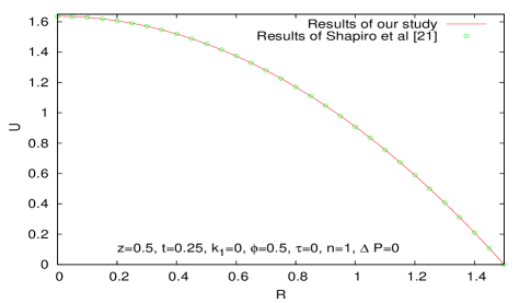
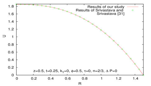
$~{}~{}~{}~{}~{}~{}~{}~{}~{}~{}~{}~{}~{}~{}~{}~{}~{}(a)~{}~{}~{}~{}~{}~{}~{}~{}~{}~{}~{}~{}~{}~{}~{}~{}~{}~{}~{}~{}~{}~{}~{}~{}~{}~{}~{}~{}~{}~{}~{}~{}~{}~{}~{}~{}~{}~{}~{}~{}~{}~{}~{}~{}~{}~{}~{}~{}~{}~{}~{}~{}~{}~{}~{}~{}~{}~{}~{}~{}~{}~{}~{}~{}~{}~{}~{}(b)~{}~{}~{}~{}~{}~{}~{}~{}~{}$

Figure 2: Variation of axial velocity in the radial direction at Z=0.5, (a) Newtonian fluid, (b) Shear-thinning fluid

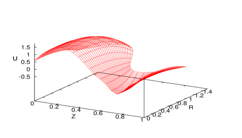
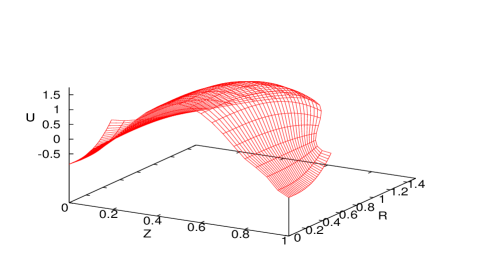
$~{}~{}~{}~{}~{}~{}~{}~{}~{}~{}~{}~{}~{}~{}~{}~{}~{}(a)~{}~{}~{}~{}~{}~{}~{}~{}~{}~{}~{}~{}~{}~{}~{}~{}~{}~{}~{}~{}~{}~{}~{}~{}~{}~{}~{}~{}~{}~{}~{}~{}~{}~{}~{}~{}~{}~{}~{}~{}~{}~{}~{}~{}~{}~{}~{}~{}~{}~{}~{}~{}~{}~{}~{}~{}~{}~{}~{}~{}~{}~{}~{}~{}~{}~{}~{}(b)~{}~{}~{}~{}~{}~{}~{}~{}~{}$
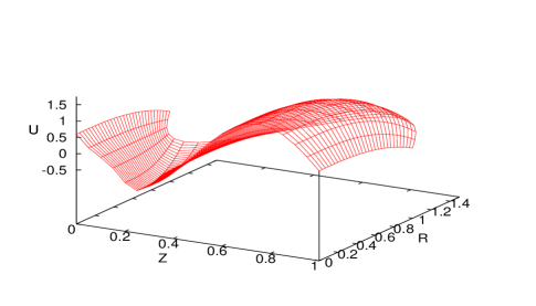
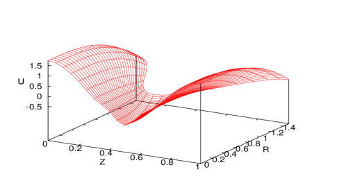
$~{}~{}~{}~{}~{}~{}~{}~{}~{}~{}~{}~{}~{}~{}~{}~{}~{}(c)~{}~{}~{}~{}~{}~{}~{}~{}~{}~{}~{}~{}~{}~{}~{}~{}~{}~{}~{}~{}~{}~{}~{}~{}~{}~{}~{}~{}~{}~{}~{}~{}~{}~{}~{}~{}~{}~{}~{}~{}~{}~{}~{}~{}~{}~{}~{}~{}~{}~{}~{}~{}~{}~{}~{}~{}~{}~{}~{}~{}~{}~{}~{}~{}~{}~{}~{}(d)~{}~{}~{}~{}~{}~{}~{}~{}~{}$

Figure 3: Aerial view of the velocity distribution at different instants of time, when $n=2/3,~{}k_{1}=0,~{}\Delta P=0,~{}\tau=0.1,~{}\phi=0.5$ for a non-Newtonian fluid of shear thinning type (a) t=0.0 (b) t=0.25 (c) t=0.5 (d) t=0.75

Theoretical estimates of different physical quantities that are of relevance to the physiological problem of blood flow in the micro-circulatory system have been obtained on the basis of the present study. For this purpose, the following data that are valid in the physiological range [15, 17, 41, 53] have been used:
$a_{0}=10~{}to~{}60\mu m$, $\phi=$ 0.1  to  0.9, $\frac{a_{0}}{\lambda}=0.01~{}to~{}0.02$, $\Delta P=-300~{}to~{}50$;  $\tau=0.0$  to  0.2; Q=0  to 2, n= $\frac{1}{3}$ to 2. The value of $k_{1}$ for the non-uniform geometry of the micro-vessel, has been chosen to match with physiological system. Thus for arterioles, which are of converging type, the width of the outlet of one wave length has been taken to be $25\%$ less than that of the inlet; in the case of diverging vessels (e.g. venules), the width of the outlet of one wave length has been taken $25\%$ more than that of the inlet.

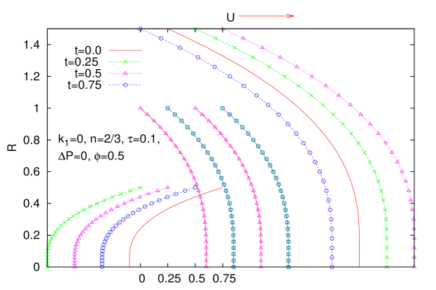
Figure 4: Velocity distribution at different instants of time.

4.1 Distribution of Velocity

For different values of the amplitude ratio $\phi$, flow index number n, $k_{1}$ and $\tau$, Figs. 2-6 present the distribution of axial velocity of blood in the cases of free pumping, pumping and co-pumping zones. Fig. 2 shows that the results computed on the basis of our study for the particular case of a Newtonian fluid and shear-thinning fluid ($n=2/3$) tally well with the results reported by Shapiro et al. [21] and Srivastava and Srivastava [31], respectively when the amplitude ratio $\phi=0.5$. Since the velocity profiles along with the radius of the blood vessels change with time, we have investigated the distribution of velocity at a time interval of a quarter of a wave period. Fig. 3 gives us the aerial view of a few typical axial velocity distributions for a Newtonian fluid and a shear-thinning fluid (n=2/3) flowing in uniform micro-vessels, while Fig. 4 presents the velocity distribution in a vessel at different instants of time. Fig. 5 reveals that at any instant of time, there exists a retrograde flow region. However, the forward flow region is predominant in this case, since the time-averaged flow rate is positive. For a shear-thinning fluid (n=2/3), the present study indicates that there exist two stagnation points on the axis. For example, at time t=0.25, one of the stagnation points lies between Z=0.0 and Z=0.25, while the other lies between Z=0.75 and Z=1.0. Similar observations were made numerically by Takabatake and Ayukawa [28] for a Newtonian fluid. Figs. 5(a)-(b) depict that in both the regions, as $\tau$ increases, the magnitude of velocity decreases for both types of fluids mentioned above. It can be observed from Fig. 5(c-d) that for a Herschel-Bulkley fluid (with n=2/3) when $\Delta P=0$, the velocity in both the regions of backward and forward flows is enhanced as the value of $\phi$ increases in the interval $0<\phi<0.6$, but beyond $\phi=0.6$, the velocity in the backward flow region decreases with $\phi$ increasing. These observations (cf. Figs. 5(c,d)) are in contrast to the case of two dimensional channel flow.

$~{}~{}~{}~{}~{}~{}~{}~{}~{}~{}~{}~{}~{}~{}~{}~{}~{}~{}~{}~{}~{}~{}~{}~{}(a)~{}~{}~{}~{}~{}~{}~{}~{}~{}~{}~{}~{}~{}~{}~{}~{}~{}~{}~{}~{}~{}~{}~{}~{}~{}~{}~{}~{}~{}~{}~{}~{}~{}~{}~{}~{}~{}~{}~{}~{}~{}~{}~{}~{}~{}~{}~{}~{}~{}~{}~{}~{}~{}(b)~{}~{}~{}~{}~{}~{}~{}~{}~{}~{}~{}~{}~{}~{}~{}$
$~{}~{}~{}~{}~{}~{}~{}~{}~{}~{}~{}~{}~{}~{}~{}~{}~{}~{}~{}~{}~{}~{}~{}~{}(c)~{}~{}~{}~{}~{}~{}~{}~{}~{}~{}~{}~{}~{}~{}~{}~{}~{}~{}~{}~{}~{}~{}~{}~{}~{}~{}~{}~{}~{}~{}~{}~{}~{}~{}~{}~{}~{}~{}~{}~{}~{}~{}~{}~{}~{}~{}~{}~{}~{}~{}~{}~{}~{}(d)~{}~{}~{}~{}~{}~{}~{}~{}~{}~{}~{}~{}~{}~{}~{}$
$~{}~{}~{}~{}~{}~{}~{}~{}~{}~{}~{}~{}~{}~{}~{}~{}~{}~{}~{}~{}~{}~{}~{}~{}~{}~{}~{}~{}~{}~{}~{}(e)~{}~{}~{}~{}~{}~{}~{}~{}~{}~{}~{}~{}~{}~{}~{}~{}~{}~{}~{}~{}~{}~{}~{}~{}~{}~{}~{}~{}~{}~{}~{}~{}~{}~{}~{}~{}~{}~{}~{}~{}~{}~{}~{}~{}~{}~{}~{}~{}~{}~{}~{}~{}~{}~{}~{}~{}~{}~{}~{}~{}~{}~{}~{}~{}~{}~{}~{}(f)~{}~{}~{}~{}~{}~{}~{}~{}~{}~{}~{}~{}~{}~{}~{}$

$~{}~{}~{}~{}~{}~{}~{}~{}~{}~{}~{}~{}~{}~{}~{}~{}~{}~{}~{}~{}~{}~{}~{}~{}~{}~{}~{}(g)~{}~{}~{}~{}~{}~{}~{}~{}~{}~{}~{}~{}~{}~{}~{}~{}~{}~{}~{}~{}~{}~{}~{}~{}~{}~{}~{}~{}~{}~{}~{}~{}~{}~{}~{}~{}~{}~{}~{}~{}~{}~{}~{}~{}~{}~{}~{}~{}~{}~{}~{}~{}~{}~{}~{}~{}~{}~{}~{}~{}~{}~{}~{}~{}~{}~{}~{}~{}~{}(h)~{}~{}~{}~{}~{}~{}~{}~{}~{}~{}~{}~{}~{}~{}~{}$
$~{}~{}~{}~{}~{}~{}~{}~{}~{}~{}~{}~{}~{}~{}~{}~{}~{}~{}~{}~{}~{}~{}~{}~{}~{}~{}~{}(i)~{}~{}~{}~{}~{}~{}~{}~{}~{}~{}~{}~{}~{}~{}~{}~{}~{}~{}~{}~{}~{}~{}~{}~{}~{}~{}~{}~{}~{}~{}~{}~{}~{}~{}~{}~{}~{}~{}~{}~{}~{}~{}~{}~{}~{}~{}~{}~{}~{}~{}~{}~{}~{}~{}~{}~{}~{}~{}~{}~{}~{}~{}~{}~{}~{}~{}~{}~{}~{}(j)~{}~{}~{}~{}~{}~{}~{}~{}~{}~{}~{}~{}~{}~{}~{}$
$~{}~{}~{}~{}~{}~{}~{}~{}~{}~{}~{}~{}~{}~{}~{}~{}~{}~{}~{}~{}~{}~{}~{}~{}~{}~{}~{}(k)~{}~{}~{}~{}~{}~{}~{}~{}~{}~{}~{}~{}~{}~{}~{}~{}~{}~{}~{}~{}~{}~{}~{}~{}~{}~{}~{}~{}~{}~{}~{}~{}~{}~{}~{}~{}~{}~{}~{}~{}~{}~{}~{}~{}~{}~{}~{}~{}~{}~{}~{}~{}~{}~{}~{}~{}~{}~{}~{}~{}~{}~{}~{}~{}~{}~{}~{}~{}~{}(l)~{}~{}~{}~{}~{}~{}~{}~{}~{}~{}~{}~{}~{}~{}~{}$

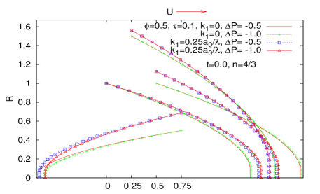
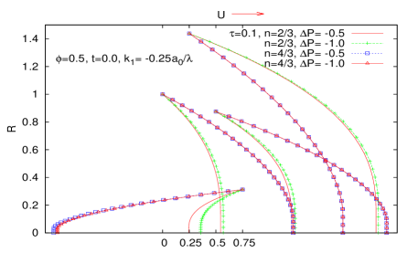
$~{}~{}~{}~{}~{}~{}~{}~{}~{}~{}~{}~{}~{}~{}~{}~{}~{}~{}~{}~{}~{}~{}~{}~{}~{}~{}~{}(m)~{}~{}~{}~{}~{}~{}~{}~{}~{}~{}~{}~{}~{}~{}~{}~{}~{}~{}~{}~{}~{}~{}~{}~{}~{}~{}~{}~{}~{}~{}~{}~{}~{}~{}~{}~{}~{}~{}~{}~{}~{}~{}~{}~{}~{}~{}~{}~{}~{}~{}~{}~{}~{}~{}~{}~{}~{}~{}~{}~{}~{}~{}~{}~{}~{}~{}~{}~{}~{}(n)~{}~{}~{}~{}~{}~{}~{}~{}~{}~{}~{}~{}~{}~{}~{}$
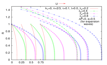
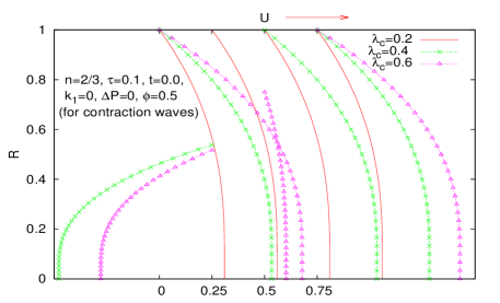
$~{}~{}~{}~{}~{}~{}~{}~{}~{}~{}~{}~{}~{}~{}~{}~{}~{}~{}~{}~{}~{}~{}~{}~{}~{}~{}~{}(o)~{}~{}~{}~{}~{}~{}~{}~{}~{}~{}~{}~{}~{}~{}~{}~{}~{}~{}~{}~{}~{}~{}~{}~{}~{}~{}~{}~{}~{}~{}~{}~{}~{}~{}~{}~{}~{}~{}~{}~{}~{}~{}~{}~{}~{}~{}~{}~{}~{}~{}~{}~{}~{}~{}~{}~{}~{}~{}~{}~{}~{}~{}~{}~{}~{}~{}~{}~{}~{}(p)~{}~{}~{}~{}~{}~{}~{}~{}~{}~{}~{}~{}~{}~{}~{}$

Figure 5: Distribution of velocity in various cases. The figures reveal that flow reversal occur due to the contraction of the wave.

In Figs. 5(e)-(k), it is worthwhile to observe the significant influence of the rheological fluid index ’n’ on the velocity distribution for flows in uniform/non-uniform vessels. These figures reveal that the parabolic nature of the velocity profiles is disturbed due to the non-Newtonian effect. Magnitude of the velocity decreases at the maximum expansion region; while in the remaining regions, a reverse trend is noticed, when there is an increase in the value of ’n’ (cf. Figs. 5(e-g,j-k)). For a converging vessel, the magnitude of the velocity is greater than that of a uniform vessel; however, for a diverging vessel, our observation is altogether different. Figs. 5(l)-(n) illustrate the influence of pressure on velocity distribution for shear thinning /shear thickening fluids. The results presented for shear-thickening fluid have been computed by taking $n=4/3$, while those for shear-thinning fluid correspond to $n=2/3$. It may be noted that in the case of a uniform/diverging vessel, if $\Delta P$ decreases, the flow reversal tends to decrease; however, for a converging tube, although there is reduction in the region of flow reversal, the change is not too significant for shear thickening fluid. It is important to mention that flow reversal takes place due to change in sign of the vorticity or the shear stress along the wavy wall.

The results corresponding to SSD wave propagation are presented in Figs. 5(o-p). It is seen that for SSD expansion waves, there is no backward flow and that the magnitude of the velocity is considerably less in this case as compared to the case of sinusoidal wave propagation (cf. Fig. 4). Moreover, as $\lambda_{c}$ increases, velocity is seen to rise except around Z=0.25 where it decreases when $\lambda_{c}$ exceeds 0.6. For SSD contraction waves, Fig. 5(n) shows that if $\lambda_{c}=0.2$, there is no backward flow within one wave length. If $\lambda_{c}>0.3$, backward flow is observed from Z=0.15 to Z=0.7.

$~{}~{}~{}~{}~{}~{}~{}~{}~{}~{}~{}~{}~{}~{}~{}~{}~{}~{}~{}~{}~{}~{}~{}~{}~{}~{}~{}(a)~{}~{}~{}~{}~{}~{}~{}~{}~{}~{}~{}~{}~{}~{}~{}~{}~{}~{}~{}~{}~{}~{}~{}~{}~{}~{}~{}~{}~{}~{}~{}~{}~{}~{}~{}~{}~{}~{}~{}~{}~{}~{}~{}~{}~{}~{}~{}~{}~{}~{}~{}~{}~{}~{}~{}~{}~{}~{}~{}~{}~{}~{}~{}~{}~{}~{}~{}~{}~{}(b)~{}~{}~{}~{}~{}~{}~{}~{}~{}~{}~{}~{}~{}~{}~{}$
$~{}~{}~{}~{}~{}~{}~{}~{}~{}~{}~{}~{}~{}~{}~{}~{}~{}~{}~{}~{}~{}~{}~{}~{}~{}~{}~{}(c)~{}~{}~{}~{}~{}~{}~{}~{}~{}~{}~{}~{}~{}~{}~{}~{}~{}~{}~{}~{}~{}~{}~{}~{}~{}~{}~{}~{}~{}~{}~{}~{}~{}~{}~{}~{}~{}~{}~{}~{}~{}~{}~{}~{}~{}~{}~{}~{}~{}~{}~{}~{}~{}~{}~{}~{}~{}~{}~{}~{}~{}~{}~{}~{}~{}~{}~{}~{}~{}(d)~{}~{}~{}~{}~{}~{}~{}~{}~{}~{}~{}~{}~{}~{}~{}$
$~{}~{}~{}~{}~{}~{}~{}~{}~{}~{}~{}~{}~{}~{}~{}~{}~{}~{}~{}~{}~{}~{}~{}~{}~{}~{}~{}(e)~{}~{}~{}~{}~{}~{}~{}~{}~{}~{}~{}~{}~{}~{}~{}~{}~{}~{}~{}~{}~{}~{}~{}~{}~{}~{}~{}~{}~{}~{}~{}~{}~{}~{}~{}~{}~{}~{}~{}~{}~{}~{}~{}~{}~{}~{}~{}~{}~{}~{}~{}~{}~{}~{}~{}~{}~{}~{}~{}~{}~{}~{}~{}~{}~{}~{}~{}~{}~{}(f)~{}~{}~{}~{}~{}~{}~{}~{}~{}~{}~{}~{}~{}~{}~{}$
$~{}~{}~{}~{}~{}~{}~{}~{}~{}~{}~{}~{}~{}~{}~{}~{}~{}~{}~{}~{}~{}~{}~{}~{}~{}~{}~{}(g)~{}~{}~{}~{}~{}~{}~{}~{}~{}~{}~{}~{}~{}~{}~{}~{}~{}~{}~{}~{}~{}~{}~{}~{}~{}~{}~{}~{}~{}~{}~{}~{}~{}~{}~{}~{}~{}~{}~{}~{}~{}~{}~{}~{}~{}~{}~{}~{}~{}~{}~{}~{}~{}~{}~{}~{}~{}~{}~{}~{}~{}~{}~{}~{}~{}~{}~{}~{}~{}(h)~{}~{}~{}~{}~{}~{}~{}~{}~{}~{}~{}~{}~{}~{}~{}$

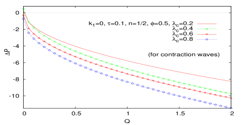
(i)

Figure 6: Pressure difference versus flow rate. It may be observed that the area of the pumping region increases when the amplitude ratio $\phi$ is enhanced. In addition, the variation of the vessel radius in both converging and diverging cases as well as SSD expansion/contraction wave modes have significant impact on the pressure difference ($\Delta$P) as well as on the volumetric flow rate (Q).

4.2 Pumping Behaviour

The pumping characteristics can be determined through the variation of time averaged flux with difference in pressure across one wave length (cf. [21]). It is known that if the flow is steady in the wave frame, the instantaneous pressure difference between two stations one wave length apart is a constant. Since the pressure gradient is a periodic function of $(Z-t)$, pressure rise per wave length $\Delta P_{\lambda}$ is equal to $\lambda$ times the time-averaged pressure gradient. In addition, the relation between the fixed frame and the wave frame flux rates turns out to be linear, as in the case of inertia-free peristaltic flow of a Newtonian fluid. From the said relation, it is possible to calculate the amount of flow pumped by peristaltic waves, even in the absence of mean pressure gradient. The region in which $\Delta P=0$ is regarded to as the free pumping zone, while the region where $\Delta P>0$ is said to be the pumping zone. The situation when $\Delta P<0$ is favourable for the flow to take place and the corresponding region is called the co-pumping zone. Since the present study is concerned with peristaltic transport of a non-Newtonian fluid, the aforesaid relationship between the pressure difference and the mean flow rate is nonlinear.

Fig. 6 illustrates the variation of volumetric flow rate of the fluid by way of propagation of peristaltic waves, for different values of the amplitude ratio $\phi$, flow index number n, as well as the parameters $\tau$ and $k_{1}$. Shapiro et al. [21] used lubrication theory to show that in the case of a Newtonian fluid, the flow rate averaged over one wave length varies linearly with pressure difference. But for our study of the peristaltic transport of a non-Newtonian fluid, the relationship between the pressure difference and the mean flow rate is found to be non-linear (cf. Figs 6). The plots presented in this figure show that for a non-Newtonian fluid, the mean flow rate Q increases as $\Delta P$ decreases. Figs. 6(a-b) indicate that area of the pumping region increases with an increase in the amplitude ratio $\phi$ for both shear thinning and shear thickening fluids. Figs. 6(c-e) illustrate the influence of the rheological parameter ‘n’ on the pumping performance in uniform/diverging/converging vessels. It may be noted that the pumping region ($\Delta P>0$) significantly increases as the value of ‘n’ increases, while in the co-pumping region ($\Delta P<0$) the pressure-difference decreases when Q exceeds a certain value. Figs. 6(f-g) show that Q is not significantly affected by the value of the parameter $\tau$ in the case of free pumping. We further find that for both shear-thinning and shear thickening fluids, pumping region increases with $\tau$ increasing. Moreover, when Q exceeds a certain critical limit, $\Delta P=0$, pressure difference decreases with an increase in $\tau$.

The effect of SSD wave propagation on pumping is revealed in Figs. 6(h-i). Unlike sinusoidal wave form, Q increases significantly in pumping, free-pumping as well as co-pumping regions for SSD expansion wave fronts as $\lambda_{c}$ increases. For SSD contraction wave fronts, our observation is altogether different from SSD expansion wave fronts. However, $Q\leq 0$ when $\Delta P<0$ for shear-thinning fluids in the case of contraction waves. This observation is in contrast to the case of sinusoidal wave propagation.

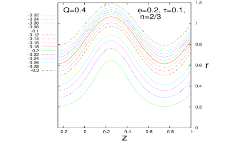
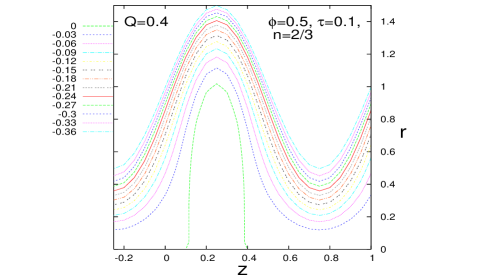
$~{}~{}~{}~{}~{}~{}~{}~{}~{}~{}~{}~{}~{}~{}~{}~{}~{}~{}~{}~{}~{}~{}~{}~{}~{}~{}~{}(a)~{}~{}~{}~{}~{}~{}~{}~{}~{}~{}~{}~{}~{}~{}~{}~{}~{}~{}~{}~{}~{}~{}~{}~{}~{}~{}~{}~{}~{}~{}~{}~{}~{}~{}~{}~{}~{}~{}~{}~{}~{}~{}~{}~{}~{}~{}~{}~{}~{}~{}~{}~{}~{}~{}~{}~{}~{}~{}(b)~{}~{}~{}~{}~{}~{}~{}~{}~{}~{}~{}~{}~{}~{}~{}~{}~{}~{}~{}~{}~{}~{}~{}~{}~{}$
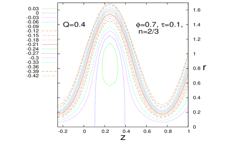
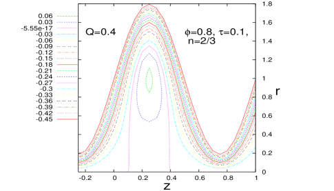
$~{}~{}~{}~{}~{}~{}~{}~{}~{}~{}~{}~{}~{}~{}~{}~{}~{}~{}~{}~{}~{}~{}~{}~{}~{}~{}~{}(c)~{}~{}~{}~{}~{}~{}~{}~{}~{}~{}~{}~{}~{}~{}~{}~{}~{}~{}~{}~{}~{}~{}~{}~{}~{}~{}~{}~{}~{}~{}~{}~{}~{}~{}~{}~{}~{}~{}~{}~{}~{}~{}~{}~{}~{}~{}~{}~{}~{}~{}~{}~{}~{}~{}~{}~{}~{}~{}(d)~{}~{}~{}~{}~{}~{}~{}~{}~{}~{}~{}~{}~{}~{}~{}~{}~{}~{}~{}~{}~{}~{}~{}~{}~{}$

Figure 7: Streamline patterns for peristaltic flow of a shear-thinning fluid for different values of $\phi$ when n=2/3, Q=0.4, $k_{1}=0$, $\tau=0$

4.3 Streamlines and Trapping

It is known that one of the important characteristics of peristaltic transport is the phenomenon of trapping. It occurs when streamlines on the central line are split to enclose a bolus of fluid particles circulating along closed streamlines in the wave frame of reference. Then the trapped bolus moves with a speed equal to the wave propagation velocity. This physical phenomenon may be responsible for the formation of thrombus in blood. Let us consider the wave frame transformations (x,y) moving with a velocity c away from a fixed frame (X,Y) such that $x=X-ct,~{}y=Y,~{}u=U-c,~{}v=V,~{}p(x,y)=P(X,Y,t),$ in which (u,v) and (U,V) are the velocity components, p and P stand for pressure in wave frame and fixed frame of reference respectively. Under the purview of the present study, Figs. 7-10 give an insight into the changes in the pattern of streamlines and trapping that occurs due to changes in the values of different parameters that govern the flow of blood in the wave frame of reference. Figs. 7 provide the streamline patterns and trapping in the case of a shear-thinning fluid for different values of $\phi$. With an increase in $\phi$, the bolus is found to appear in a distinct manner. Streamlines for different values of the fluid index ‘n’ are depicted in Fig. 8. This figure indicates that occurrence of trapping is strongly influenced by the value of the fluid index. Fig. 9 shows that trapped bolus increases in size and also that it has a tendency to move towards the boundary as the flow rate increases. Here it is important to note that the bolus appearing for small values of $\tau$ decreases in size with an increase in $\tau$ (Figs. 10).

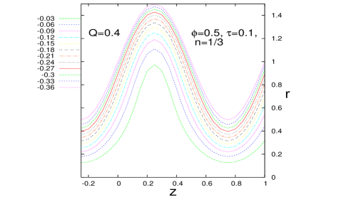
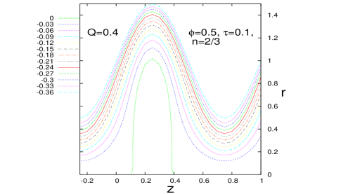
$~{}~{}~{}~{}~{}~{}~{}~{}~{}~{}~{}~{}~{}~{}~{}~{}~{}~{}~{}~{}~{}~{}~{}~{}~{}~{}~{}(a)~{}~{}~{}~{}~{}~{}~{}~{}~{}~{}~{}~{}~{}~{}~{}~{}~{}~{}~{}~{}~{}~{}~{}~{}~{}~{}~{}~{}~{}~{}~{}~{}~{}~{}~{}~{}~{}~{}~{}~{}~{}~{}~{}~{}~{}~{}~{}~{}~{}~{}~{}~{}~{}~{}~{}~{}~{}~{}(b)~{}~{}~{}~{}~{}~{}~{}~{}~{}~{}~{}~{}~{}~{}~{}~{}~{}~{}~{}~{}~{}~{}~{}~{}~{}$
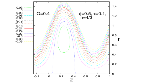
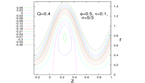
$~{}~{}~{}~{}~{}~{}~{}~{}~{}~{}~{}~{}~{}~{}~{}~{}~{}~{}~{}~{}~{}~{}~{}~{}~{}~{}~{}(c)~{}~{}~{}~{}~{}~{}~{}~{}~{}~{}~{}~{}~{}~{}~{}~{}~{}~{}~{}~{}~{}~{}~{}~{}~{}~{}~{}~{}~{}~{}~{}~{}~{}~{}~{}~{}~{}~{}~{}~{}~{}~{}~{}~{}~{}~{}~{}~{}~{}~{}~{}~{}~{}~{}~{}~{}~{}~{}(d)~{}~{}~{}~{}~{}~{}~{}~{}~{}~{}~{}~{}~{}~{}~{}~{}~{}~{}~{}~{}~{}~{}~{}~{}~{}$

Figure 8: Streamline patterns and trapping in the case of peristaltic flow for different values of the physiological fluid index ‘n’ when $\phi=0.5,~{}\tau=0.1,~{}k_{1}=0,~{}Q=0.4$. The figures show that the occurrence of trapping is highly dependent on the value of the fluid index ‘n’.

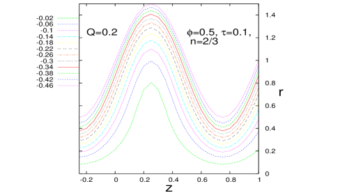
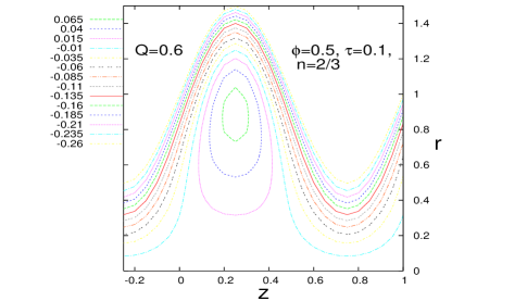
$~{}~{}~{}~{}~{}~{}~{}~{}~{}~{}~{}~{}~{}~{}~{}~{}~{}~{}~{}~{}~{}~{}~{}~{}~{}~{}~{}(a)~{}~{}~{}~{}~{}~{}~{}~{}~{}~{}~{}~{}~{}~{}~{}~{}~{}~{}~{}~{}~{}~{}~{}~{}~{}~{}~{}~{}~{}~{}~{}~{}~{}~{}~{}~{}~{}~{}~{}~{}~{}~{}~{}~{}~{}~{}~{}~{}~{}~{}~{}~{}~{}~{}~{}~{}~{}~{}(b)~{}~{}~{}~{}~{}~{}~{}~{}~{}~{}~{}~{}~{}~{}~{}~{}~{}~{}~{}~{}~{}~{}~{}~{}~{}$
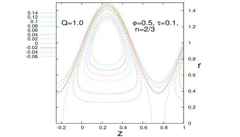
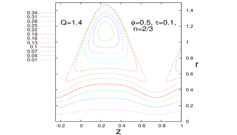
$~{}~{}~{}~{}~{}~{}~{}~{}~{}~{}~{}~{}~{}~{}~{}~{}~{}~{}~{}~{}~{}~{}~{}~{}~{}~{}~{}(c)~{}~{}~{}~{}~{}~{}~{}~{}~{}~{}~{}~{}~{}~{}~{}~{}~{}~{}~{}~{}~{}~{}~{}~{}~{}~{}~{}~{}~{}~{}~{}~{}~{}~{}~{}~{}~{}~{}~{}~{}~{}~{}~{}~{}~{}~{}~{}~{}~{}~{}~{}~{}~{}~{}~{}~{}~{}~{}~{}~{}~{}~{}~{}~{}~{}~{}(d)~{}~{}~{}~{}~{}~{}~{}~{}~{}~{}~{}~{}~{}~{}~{}~{}~{}~{}~{}~{}~{}~{}~{}~{}~{}$

Figure 9: Streamline patterns and trapping for the effect of $Q$, when $n=2/3,~{}\phi=0.5,~{}k_{1}=0,\tau=0.1$

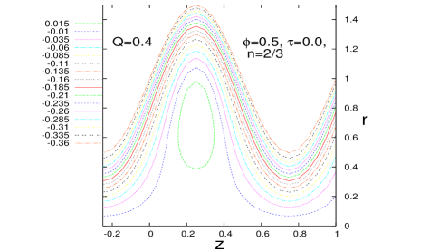
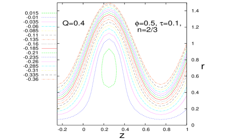
$~{}~{}~{}~{}~{}~{}~{}~{}~{}~{}~{}~{}~{}~{}~{}~{}~{}~{}~{}~{}~{}~{}~{}~{}~{}~{}~{}(a)~{}~{}~{}~{}~{}~{}~{}~{}~{}~{}~{}~{}~{}~{}~{}~{}~{}~{}~{}~{}~{}~{}~{}~{}~{}~{}~{}~{}~{}~{}~{}~{}~{}~{}~{}~{}~{}~{}~{}~{}~{}~{}~{}~{}~{}~{}~{}~{}~{}~{}~{}~{}~{}~{}~{}~{}~{}~{}(b)~{}~{}~{}~{}~{}~{}~{}~{}~{}~{}~{}~{}~{}~{}~{}~{}~{}~{}~{}~{}~{}~{}~{}~{}~{}$
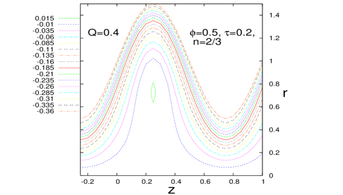
$~{}~{}~{}~{}~{}~{}~{}~{}~{}~{}~{}~{}~{}~{}~{}~{}~{}~{}~{}~{}~{}~{}~{}~{}~{}~{}~{}(c)~{}~{}~{}~{}~{}~{}~{}~{}~{}~{}~{}~{}~{}~{}~{}~{}~{}~{}~{}~{}~{}~{}~{}~{}~{}~{}~{}~{}~{}~{}~{}~{}~{}~{}~{}~{}~{}~{}~{}~{}~{}~{}~{}~{}~{}~{}~{}~{}~{}~{}~{}~{}~{}~{}~{}~{}~{}~{}~{}~{}~{}~{}~{}(d)~{}~{}~{}~{}~{}~{}~{}~{}~{}~{}~{}~{}~{}~{}~{}~{}~{}~{}~{}~{}~{}~{}~{}~{}~{}~{}~{}~{}~{}$

Figure 10: Streamline patterns for different values of $\tau$ in the case of peristaltic flow when $n=2/3,~{}\phi=0.5,~{}k_{1}=0,~{}Q=0.4$. It may be observed that the size of the bolus reduces with the increase in the value of $\tau$. The bolus totally disappears for $\tau\geq 0.3$.

4.4 Distribution of Wall Shear Stress

If the shear stress generated on the wall of a blood vessel exceeds a certain limit, the constituents of blood are likely to be damaged. The magnitude of the wall shear stress has a vital role in the process of molecular convection at high Prandtl or Schmidt number [54]. In view of these observations, it is important to study the shear stress that is developed during the hemodynamical flow of blood in small arteries. The wall shear stress distributions for the present study are plotted in Figs. 11 under varied conditions. The distributions of wall shear stress at four different time instants during one complete wave period have been presented in Fig. 11(a). It may be observed from this figure that at each of these instants of time, there exist two peaks in the wall shear stress distribution, with a gradual ramp in between; however, negative peak of wall shear stress $\tau_{min}$ is not as large as the maximum wall shear stress $\tau_{max}$. The transition from $\tau_{min}$ to $\tau_{max}$ of wall shear takes place in some zone between the minimum and maximum radii of the vessel. At the location where the maximum occlusion occurs, wall shear stress along with the pressure is maximum. Since the pressure gradient to the left of this location takes a positive value, the local instantaneous flow will take place towards the left of $\tau_{max}$. This may lead to some serious consequences. For example, if the shear rate at the crest exceeds some limit, a dissolving wavy wall will have a tendency to level out. Moreover, some bio-chemical reaction between the wall material and the constituents of blood may set in. As a result of this, the products of the chemical reaction may be deposited on the endothelium and consequently wall amplitude may increase at a rapid rate. This is likely to lead to clogging of the blood vessel.

$~{}~{}~{}~{}~{}~{}~{}~{}~{}~{}~{}~{}~{}~{}~{}~{}~{}~{}~{}~{}~{}~{}~{}~{}~{}~{}~{}(a)~{}~{}~{}~{}~{}~{}~{}~{}~{}~{}~{}~{}~{}~{}~{}~{}~{}~{}~{}~{}~{}~{}~{}~{}~{}~{}~{}~{}~{}~{}~{}~{}~{}~{}~{}~{}~{}~{}~{}~{}~{}~{}~{}~{}~{}~{}~{}~{}~{}~{}~{}~{}~{}~{}~{}~{}~{}~{}~{}~{}~{}~{}~{}~{}~{}~{}~{}~{}~{}(b)~{}~{}~{}~{}~{}~{}~{}~{}~{}~{}~{}~{}~{}~{}~{}$
$~{}~{}~{}~{}~{}~{}~{}~{}~{}~{}~{}~{}~{}~{}~{}~{}~{}~{}~{}~{}~{}~{}~{}~{}~{}~{}~{}(c)~{}~{}~{}~{}~{}~{}~{}~{}~{}~{}~{}~{}~{}~{}~{}~{}~{}~{}~{}~{}~{}~{}~{}~{}~{}~{}~{}~{}~{}~{}~{}~{}~{}~{}~{}~{}~{}~{}~{}~{}~{}~{}~{}~{}~{}~{}~{}~{}~{}~{}~{}~{}~{}~{}~{}~{}~{}~{}~{}~{}~{}~{}~{}~{}~{}~{}~{}~{}~{}(d)~{}~{}~{}~{}~{}~{}~{}~{}~{}~{}~{}~{}~{}~{}~{}$
$~{}~{}~{}~{}~{}~{}~{}~{}~{}~{}~{}~{}~{}~{}~{}~{}~{}~{}~{}~{}~{}~{}~{}~{}~{}~{}~{}(e)~{}~{}~{}~{}~{}~{}~{}~{}~{}~{}~{}~{}~{}~{}~{}~{}~{}~{}~{}~{}~{}~{}~{}~{}~{}~{}~{}~{}~{}~{}~{}~{}~{}~{}~{}~{}~{}~{}~{}~{}~{}~{}~{}~{}~{}~{}~{}~{}~{}~{}~{}~{}~{}~{}~{}~{}~{}~{}~{}~{}~{}~{}~{}~{}~{}~{}~{}~{}~{}(f)~{}~{}~{}~{}~{}~{}~{}~{}~{}~{}~{}~{}~{}~{}~{}$

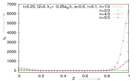
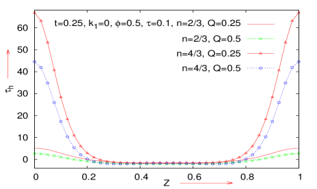
$~{}~{}~{}~{}~{}~{}~{}~{}~{}~{}~{}~{}~{}~{}~{}~{}~{}~{}~{}~{}~{}~{}~{}~{}~{}~{}~{}(g)~{}~{}~{}~{}~{}~{}~{}~{}~{}~{}~{}~{}~{}~{}~{}~{}~{}~{}~{}~{}~{}~{}~{}~{}~{}~{}~{}~{}~{}~{}~{}~{}~{}~{}~{}~{}~{}~{}~{}~{}~{}~{}~{}~{}~{}~{}~{}~{}~{}~{}~{}~{}~{}~{}~{}~{}~{}~{}~{}~{}~{}~{}~{}~{}~{}~{}~{}~{}~{}(h)~{}~{}~{}~{}~{}~{}~{}~{}~{}~{}~{}~{}~{}~{}~{}$
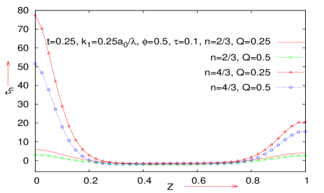
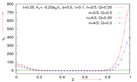
$~{}~{}~{}~{}~{}~{}~{}~{}~{}~{}~{}~{}~{}~{}~{}~{}~{}~{}~{}~{}~{}~{}~{}~{}~{}~{}~{}(i)~{}~{}~{}~{}~{}~{}~{}~{}~{}~{}~{}~{}~{}~{}~{}~{}~{}~{}~{}~{}~{}~{}~{}~{}~{}~{}~{}~{}~{}~{}~{}~{}~{}~{}~{}~{}~{}~{}~{}~{}~{}~{}~{}~{}~{}~{}~{}~{}~{}~{}~{}~{}~{}~{}~{}~{}~{}~{}~{}~{}~{}~{}~{}~{}~{}~{}~{}~{}~{}(j)~{}~{}~{}~{}~{}~{}~{}~{}~{}~{}~{}~{}~{}~{}~{}$
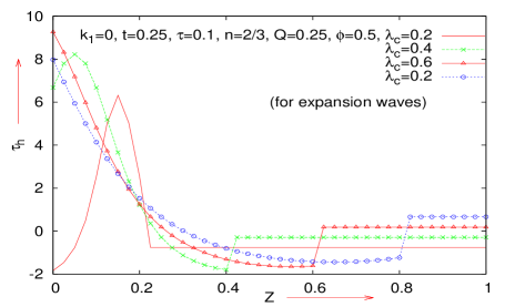
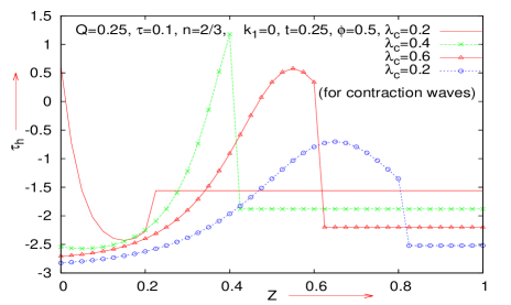
$~{}~{}~{}~{}~{}~{}~{}~{}~{}~{}~{}~{}~{}~{}~{}~{}~{}~{}~{}~{}~{}~{}~{}~{}~{}~{}~{}(k)~{}~{}~{}~{}~{}~{}~{}~{}~{}~{}~{}~{}~{}~{}~{}~{}~{}~{}~{}~{}~{}~{}~{}~{}~{}~{}~{}~{}~{}~{}~{}~{}~{}~{}~{}~{}~{}~{}~{}~{}~{}~{}~{}~{}~{}~{}~{}~{}~{}~{}~{}~{}~{}~{}~{}~{}~{}~{}~{}~{}~{}~{}~{}~{}~{}~{}~{}~{}~{}(l)~{}~{}~{}~{}~{}~{}~{}~{}~{}~{}~{}~{}~{}~{}~{}$

Figure 11: Wall shear stress distribution in different situations. Wall shear stress attains its maximum/minimum at the location where the radius of the vessel is smallest/largest.

The peaks of the wall shear stress distribution on both sides of $\tau_{max}$ are small and hence the local instantaneous flow will occur in the direction of propagation of the peristaltic waves. For a Herschel-Bulkley fluid, Figs. 11(b-c) show that in the contracting region where occlusion takes place, there is a remarkable increase in the wall shear stress due to an increase in the value of $\phi$ for both shear-thinning and shear-thickening fluids. With an increase in $\phi$, magnitude of $\tau_{min}$ increases in the expanding region for shear-thinning/shear-thickening fluids, although the effect is not very prominent. It may be observed from Fig. 11(d) that $\tau_{max}$ increases with increase in $\tau$, while $\tau$ has little effect on $\tau_{min}$.

The quantum of influence of the rheological fluid index ’n’ on the distribution of wall shear stress is shown in Figs. 11(e-g) for uniform/non-uniform blood vessels. In all types of vessels studied here, $\tau_{max}$ increases with increase in ‘n’. It is very important to mention that the difference of shear stress between the outlet and the inlet in the case of a converging vessel is exceedingly large in comparison to the case of a diverging vessel. As the time averaged flow rate increases, Figs. 11(h-j) indicate very clearly that the wall shear stress tends to decrease for all types of vessels examined here. One can observe from Figs. 11(k-l) that $\tau_{h}$ changes its values within the region of SSD wave activation; beyond this, it maintains a constant value.

5 Summary and Conclusion

The present paper deals with a study of the peristaltic motion of blood in the micro-circulatory system, by taking into account the non-Newtonian nature of blood and the non-uniform geometry of the micro-vessels, e.g. arterioles and venules. The non-Newtonian viscosity of blood is considered to be of Herschel-Bulkley type. The effects of amplitude ratio, mean pressure gradient, yield stress and the rheological fluid index n on the distribution of velocity and wall shear stress as well as on the pumping phenomena, formation of the streamline pattern and the occurrence of trapping are investigated under the purview of the lubrication theory. Experimental observations have revealed that in the case of roller pumps, the fluid elements are prone to significant damage. Moreover, during the process of transportation of fluids in living structures executed by using arthro-pumps, the fluid particles are likely to be appreciably damaged. Qualitative and quantitative studies of the present problem for the wall shear stress have a significant bearing on extracorporeal circulation. When the heart-lung machine is used for patient care, the erythrocytes of blood are likely to be damaged. Thus the present study bears the potential of significant application in biomedical engineering and technology.

The study reveals that at any instant of time, there is a retrograde flow region for Herschel-Bulkley type of non-Newtonian fluids like blood when $\Delta P\leq 0$. The regions of forward/retrograde flow advance at a faster rate, if the values of n and $\phi$ are raised. In the case of a uniform/diverging tube, the flow reversal decreases when $\Delta P$ tends to be negative; however, for a converging tube such an observation is not very prominent. In addition, this study shows that non-uniform geometry of the vessel affects quite significantly the distributions of velocity and the wall shear stress as well as pumping and other flow characteristics. It is also observed that the amplitude ratio $\phi$ and the rheological fluid index ‘n’ are very sensitive parameters that change the peristaltic pumping characteristics and the distribution of velocity and wall shear tress. The parabolic nature of the velocity profiles is also significantly disturbed by the numerical value of the rheological fluid index ‘n’.

From the present study we may conclude that for the peristaltic flow of blood through propagation of SSD expansion waves, the pumping performance is better than that in the case of sinusoidal wave propagation and that the backward flow region is totally absent in SSD expansion wave propagation mode. On the basis of this study one may also draw the conclusion that backward flow originates due to the contraction of vessels.

Acknowledgment: The authors wish to convey their thanks to all the reviewers (anonymous) for their comments and suggestions based upon which the present version of the manuscript has been prepared. One of the authors, S. Maiti, is thankful to the Council of Scientific and Industrial Research (CSIR), New Delhi and the University Grants Commission (UGC), New Delhi for awarding an SRF and the Dr. D. S. Kothari Post Doctoral Fellowship respectively during this investigation. The other author, Prof. J. C. Misra, wishes to express his deep sense of gratitude to Professor (Dr.) Manoj Ranjan Nayak, President of the Sikha O Anusandhan University, Bhubaneswar for providing a congenial environment and facilities for doing research.

References

- [1] Chen, G.Q., Wu, Z., Taylor dispersion in a two-zone packed tube, Int. J. Heat Mass Transfer 55(1-3), (2012) 43-52.
- [2] Jaggy C., Lachat M., Leskosek B., Zünd G. and Turina M., Affinity pump system: a new peristaltic blood pump for cardiopulmonary bypass, Perfusion 15(1) (2000), 77-83.
- [3] Hansbro S. D., Sharpe D. A., Catchpole R., Welsh K. R., Munsch C. M., McGoldrick J. P. and Kay P. H., Haemolysis during cardiopulmonary bypass: an in vivo comparison of standard roller pumps, nonocclusive roller pumps and centrifugal pumps, Perfusion 14(1) (1999), 3-10.
- [4] Nisar A., Afzulpurkar N., Mahaisavariya B. and Tuantranont A., MEMS-based micropumps in drug delivery and biomedical applications, Sens. Actuators B 130 (2008), 917–942.
- [5] Misra J. C. and Pandey S. K., Peristaltic transport of particle-fluid suspension in a cylindrical tube, Comput. Math. Appl 28(4) (1994), 131-145.
- [6] Misra J. C. and Pandey S. K., Peristaltic transport of a non-Newtonian fluid with a peripheral layer, Int. J. Eng. Sci. 37 (1999), 1841-1858.
- [7] Misra J. C. and Maiti S., Peristaltic transport of rheological fluid: model for movement of food bolus through esophagus, Appl. Math. Mech. 33(3) (2012), 15-32.
- [8] Misra J. C. and Pandey S. K. Peristaltic flow of a multi layered power-law fluid through a cylindrical tube. Int. J. Eng. Sci. 39 (2001), 387-402.
- [9] Misra J. C. and Maiti S., Peristaltic pumping of blood through small vessels of varying cross-section, Trans. ASME J. App. Mech. 22(8) (2012), 061003 (19 pages).
- [10] Misra J. C. and Pandey S. K., Peristaltic transport of blood in small vessels: study of a mathematical model, Compu. Math. Appl 43 (2002), 1183-1193.
- [11] Misra J. C. and Pandey S. K., Peristaltic transport of physiological fluids, in Biomathematics: Modelling and Simulation, J.C. Misra (Ed.), World Scientific Publishing Company, London/USA/Singapore, 167-193, (2006).
- [12] Misra J. C., Maiti S.. and Shit G. C, Peristaltic Transport of a Physiological Fluid in an Asymmetric Porous Channel in the Presence of an External Magnetic Field, J. Mech. Med. Biol. 8(4) (2008), 507-525.
- [13] Maiti S., Misra J. C., Peristaltic Flow of a Fluid in a Porous Channel: a Study Having Relevance to Flow of Bile, Int. J. Eng. Sci. 49 (2011), 950-966.
- [14] Maiti S., Misra J. C., Peristaltic Transport of a Couple Stress Fluid: Some Applications to Hemodynamics, J. Mech. Med. Biol. 12(3) (2012), 1250048 (21 pages).
- [15] Guyton A. C. and Hall J. E., Text Book of Medical Physiology, Elsevier: Saunders Co (2006).
- [16] Jaffrin M. Y. and Shapiro A. H., Peristaltic pumping, Annu. Rev. Fluid Mech. 3 (1971), 13-36.
- [17] Srivastava L. P. and Srivastava V. P., Peristaltic transport of blood: Casson model II, J. Biomech. 17 (1984), 821-829.
- [18] Vajravelu K., Sreenadh S., Lakshminarayana P., The influence of heat transfer on peristaltic transport of a Jeffrey fluid in a vertical porous stratum, Commun. Non-linear Sci. Numer. Simul. 16 (2011), 3107-3125.
- [19] Hayat T., Saleem N. and Ali N., Effect of induced magnetic field on peristaltic transport of a Carreau fluid, Commun. Non-linear Sci. Numer. Simul. 15 (2010), 2407-2423.
- [20] Fung Y. C. and Yih C. S., Peristaltic Transport, J. Appl. Mech. 35 (1968), 669-675.
- [21] Shapiro A. H. Jaffrin M. Y. and Weinberg S. L., Peristaltic pumping with long wavelength at low Reynolds number, J. Fluid Mech. 37 (1969), 799-825.
- [22] Tsiklauri D. and Beresnev I., Non-Newtonian effects in the peristaltic flow of a Maxwell fluid, Phys. Rev. E 64 (2001), 036303.
- [23] Mishra M. and Rao A. R., Peristaltic transport in a channel with a porous peripheral layer: model of a flow in gastrointestinal tract, J. Biomech. 38 (2005), 779-789.
- [24] Yaniv S., Jaffa A. J., Eytan O. and Elad D., Simulation of embryo transport in a closed uterine cavity model, Euro. J. Obst. Gynecol. Reprodu. Biol. 144S (2009), S50-S60.
- [25] Jimenez-Lozano J., Sen M. and Dunn P. F., Particle motion in unsteady two-dimensional peristaltic flow with application to the ureter, Phys. Rev. E 79 (2009), 041901.
- [26] Nadeem S. and Akbar N. S., Influence of heat transfer on a peristaltic transport of Herschel–Bulkley fluid in a non-uniform inclined tube, Commun. Non-linear Sci. Numer. Simul. 14 (2009), 4100-4113.
- [27] Pandey S. K. and Chaube M.K., Peristaltic flow of a micropolar fluid through a porous medium in the presence of an external magnetic field, Commun. Non-linear Sci. Numer. Simulat. 16 (2011), 3591-3601.
- [28] Takabatake S. and Ayukawa K., Numerical study of two-dimensional peristaltic flows, J. Fluid Mech. 122 (1982), 439-465.
- [29] Jimenez-Lozano J. and Sen M., Particle dispersion in two-dimensional peristaltic flow, Phys. Fluids 22 (2010), 043303.
- [30] Bohme G. and Friedrich R., Peristaltic transport of viscoelastic liquids, J. Fluid Mech. 128 (1983), 109-122
- [31] Srivastava L. M. and Srivastava V. P., Peristaltic transport of a non-Newtonian fluid: appliocations to the vas deferens and small intestine, Annals. Biomed. Eng. 13 (1985), 137-153.
- [32] Provost A. M. and Schwarz W. H., A theoretical study of viscous effects in peristaltic pumping, J. Fluid Mech. 279 (1994), 177-195.
- [33] Chakraborty S., Augmentation of peristaltic micro-flows through electro-osmotic mechanisms, J. Phys. D: Appl. Phys. 39 (2006), 5356-5363.
- [34] Rand P. W., Lacombe E., Hunt H. E. and Austin W. H., Viscosity of normal blood under normothermic and hypothermic conditions, J. Appl. Physiol. 19 (1964 ), 117-122.
- [35] Bugliarello G., Kapur C. and Hsiao G., The profile viscosity and other characteristics of blood flow in a non-uniform shear field, Proc IVth International Congress on Rheology, 4 (1965), Symp of Biorheol (Ed. Copley A L), 351-370, Interscience, New York
- [36] Chien S., Usami S., Taylor H. M., Lundberg J. L. and Gregerson M. T., Effects of hematocrit and plasma proteins on human blood rheology at low shear rates, J. Appl. Physiol. 21 (1966), 81-87.
- [37] Charm S. E. and Kurland G. S., Viscometry of human blood for shear rates of 0-100, 000 sec-1, Nature 206 (1965), 617-629.
- [38] Charm S. E. and Kurland G. S., Blood Flow and Microcirculation, New York: John Wiley (1974).
- [39] Merrill F. W., Benis A. M., Gilliland E. R., Sherwood T. K. and Salzman E. W., Pressure flow relations of human blood in hollow fibers at low flow rates, J. Appl. Physiol. 20 (1965), 954-967.
- [40] Scott-Blair G. W. and Spanner D. C., An Introduction to Bioreheology, Elsevier, Amsterdam (1974).
- [41] Fung Y. C., Biomechanics, Mechanical Properties of Living Tissues, Springer Verlag, New York (1981).
- [42] White F. M., Viscous Fluid Flow, McGraw-Hill, New York (1974).
- [43] Xue H., The modified Casson’s equation and its application to pipe flows of shear thickening fluid, Acta Mech. Sinica 21 (2005), 243-248.
- [44] Wiedman M. P., Dimensions of blood vessels from distributing artery to collecting vein, Circ. Research 12 (1963), 375-381.
- [45] Wiederhielm C. A., Analysis of small vessel function, In Physical Bases of Circulatory Transport: Regulation and Exchange, edited by Reeve, E. B. and Guyton, A. C., 313-326 W. B.Saunders, Philadelphia (1967).
- [46] Lee J. S. and Fung Y. C., Flow in non-uniform small blood vessels, Microvas. Research 3 (1971), 272-287.
- [47] Gupta B. B. and Seshadri V. J., Peristaltic pumping in non-uniform tubes, J. Biomech. 9 (1976), 105-109.
- [48] Srivastava L. M. and Srivastava V. P., Peristaltic transport of a physio-logical fluid, part I: Flow in non-uniform geometry, Biorheol 20 (1983), 153-166.
- [49] Malek J., Necas J. and Rajagopal K. R., Global existence of solutions for fluids with pressure and shear dependent viscosities, Appl. Math. Lett. 15 (2002), 961-967.
- [50] Herschel W. H. and Bulkley R., Konsistenzmessungen von Gummi-Benzollosungen, Kolloid Zeitschrift 39 (1926), 291-300.
- [51] Sahu K. C., Valluri P., Spelt P. D. M., and Matar O. K., Linear instability of pressure-driven channel flow of a Newtonian and a Herschel-Bulkley fluid, Phys. Fluids 19 (2007), 122101.
- [52] Lardner T. J. and Shack W. J., Cilia transport, Bull. Math. Biol 34 (1972), 325-335.
- [53] Barbee K. A., Davies P. F. and Lal R., Shear stress-induced reorganization of the surface topography of living endothelial cells imaged by atomic force microscopy, Circul Research 74 (1994 ), 163-171.
- [54] Higdon J. J. L., Stokes flow in arbitrary two-dimensional domains: shear flow over ridges and cavities, J. Fluid Mech. 159 (1985), 195-226.