Holographic View on Quantum Correlations and Mutual Information between Disjoint Blocks of a Quantum Critical System.

Abstract

In ($d+1$) dimensional Multiscale Entanglement Renormalization Ansatz (MERA) networks, tensors are connected so as to reproduce the discrete, ($d+2$) holographic geometry of Anti de Sitter space (AdS_d+2) with the original system lying at the boundary. We analyze the MERA renormalization flow that arises when computing the quantum correlations between two disjoint blocks of a quantum critical system, to show that the structure of the causal cones characteristic of MERA, requires a transition between two different regimes attainable by changing the ratio between the size and the separation of the two disjoint blocks. We argue that this transition in the MERA causal developments of the blocks may be easily accounted by an AdS_d+2 black hole geometry when the mutual information is computed using the Ryu-Takayanagi formula. As an explicit example, we use a BTZ AdS₃ black hole to compute the MI and the quantum correlations between two disjoint intervals of a one dimensional boundary critical system. Our results for this low dimensional system not only show the existence of a phase transition emerging when the conformal four point ratio reaches a critical value but also provide an intuitive entropic argument accounting for the source of this instability. We discuss the robustness of this transition when finite temperature and finite size effects are taken into account.

1 Introduction

Entanglement entropy (EE) is by now regarded as a valuable tool to witness the amount of entanglement in quantum field theories and many body systems. By partitioning a given system ${\mathcal{S}}$ into two complementary sets ${\mathcal{A}}$ and $\widetilde{\mathcal{A}}$ such that ${\mathcal{S}}={\mathcal{A}}\cup\widetilde{\mathcal{A}}$, the reduced density matrix $\rho_{\mathcal{A}}$ (i.e, the density matrix for an observer accessing only the degrees of freedom of the subsystem ${\mathcal{A}}$), is obtained by tracing the full density matrix $\rho$ over the degrees of freedom contained in $\widetilde{\mathcal{A}}$ i.e, $\rho_{\mathcal{A}}=\rm{Tr}_{\widetilde{\mathcal{A}}}(\rho)$. The EE accounts for the amount of quantum correlations between the complementary regions ${\mathcal{A}}$ and $\widetilde{\mathcal{A}}$ and is defined as the von Neumann entropy of $\rho_{\mathcal{A}}$,

$$S_{\mathcal{A}}=-\rm{Tr}(\rho_{\mathcal{A}}\log\rho_{\mathcal{A}})~{}.$$ (1)

A standard approach to compute the entanglement entropy makes use of the replica trick Holzhey94 ; cargliozzi ; Calabrese04 . The replica trick may be applied when the density matrix for the full system is represented by a path integral (as in the vacuum or in a thermal state); then, one can rather easily obtain the EE (1) of the subsystem ${\mathcal{A}}$ from the knowledge of,

$$S_{\mathcal{A}}=-\frac{\partial}{\partial n}{\rm Tr}\rho_{\mathcal{A}}^{n}|_{n=1}~{}.$$ (2)

In Calabrese04 , it has been shown that, for $d=1$ quantum critical models, ${\rm Tr}\rho_{\mathcal{A}}^{n}=c_{n}(\ell_{\mathcal{A}}/\epsilon)^{-(c/6)(n-1/n)}$, where $\ell_{\mathcal{A}}$ is the length of the interval ${\mathcal{A}}$, $c$ is the central charge of the conformal field theory (CFT) describing the given system at criticality and $\epsilon$ is an ultraviolet cutoff. Using (2), one obtains that the EE is given by,

$$S_{\mathcal{A}}=\frac{c}{3}\log\left(\frac{\ell_{\mathcal{A}}}{\epsilon}\right)+s_{1}~{},$$ (3)

where $s_{1}$ is a non universal constant.

Using an alternative approach based on holography Ryu and Takayanagi (RT) derived a celebrated formula yielding the EE of the region ${\mathcal{A}}$ provided that the (boundary) conformal field theory describing the critical system admits an holographic gravity dual Ryu106 ; Ryu06 . In the RT approach, the EE is obtained from the computation of a minimal surface in the dual higher dimensional gravitational geometry (bulk theory); as a result, the entanglement entropy $S_{\mathcal{A}}$ in a CFT_d+1 is given by the celebrated area law relation,

$$S_{\mathcal{A}}=\frac{{\rm Area}(\gamma_{\mathcal{A}})}{4G^{(d+2)}_{N}}~{},$$ (4)

where $d$ is the spatial dimension of the boundary CFT, $\gamma_{\mathcal{A}}$ is the $d$-dimensional static minimal surface in AdS_d+2 whose boundary and area are given by $\partial{\mathcal{A}}$ and ${\rm Area}(\gamma_{\mathcal{A}})$, respectively. $G^{(d+2)}_{N}$ is the $d+2$ dimensional Newton constant. The RT proposal is physically appealing since looking for the minimal surface $\gamma_{\mathcal{A}}$ separating the degrees of freedom contained in region ${\mathcal{A}}$ from those contained in $\widetilde{\mathcal{A}}$ amounts to search for the severest entropy bound on the information hidden in the AdS_d+2 region related with $\widetilde{\mathcal{A}}$. For $d=1$, eq. (4) becomes Ryu106 ,

$$S_{\mathcal{A}}=\frac{{\rm Length}(\gamma_{\mathcal{A}})}{4G^{(3)}_{N}}~{}.$$ (5)

Although the RT formula has not been rigorously proven its validity is supported by very comforting evidence. For instance, one may show headrick07 that it provides a simple tool to prove the strong subadditivity of EE, i.e given two regions $A$ and $B$,

$$S_{A}+S_{B}\geq S_{A\cup B}+S_{A\cap B}~{};$$ (6)

furthermore, eq. (4) together with (6) may be used also (at least in the context of strongly coupled gauge theories, i.e at a t’Hooft coupling $\lambda\gg 1$) to derive the concavity property of coplanar Wilson loops defined on curves $C_{A}=\partial A$ and $C_{B}=\partial B$ lying in the same two dimensional plane. Namely,

$$\left\langle W(C_{A})\right\rangle\left\langle W(C_{B})\right\rangle\leq\left\langle W(C_{A\cup B})\right\rangle\left\langle W(C_{A\cap B})\right\rangle~{},$$ (7)

where $C_{A\cup B}=\partial(A\cup B)$ and $C_{A\cap B}=\partial(A\cap B)$. To derive (7) one only needs to note that, from the Maldacena conjecture AdSCFTbible00 , the expectation value of a Wilson loop defined along a curve $C$ is related to the area of the minimal surface $\gamma$ bounded by $C$ by,

$$\left\langle W(C)\right\rangle\simeq\exp(-\sqrt{\lambda}\rm{Area}(\gamma))~{}.$$ (8)

If in (8) one takes $C=C_{A}=\partial A$ and $\gamma=\gamma_{A}$, using (4) one can establish, up to a constant that $S_{A}\sim-\log\left\langle W(\partial A)\right\rangle$. Similar arguments yield $S_{B}\sim-\log\left\langle W(\partial B)\right\rangle$, $S_{A\cup B}\sim-\log\left\langle W(\partial(A\cup B))\right\rangle$ and $S_{A\cap B}\sim-\log\left\langle W(\partial(A\cap B))\right\rangle$. As a result, using (6), one gets (7).

The minimal curves used in the RT formula, allow also to compute the two point functions of conformal primary operators of ${\rm CFT}_{d+1}$ with an holographic gravity dual that is an asymptotically ${\rm AdS}_{d+2}$ space-time. The holographic computation of the correlation functions of these operators yields susskind98 ,

$$\langle{\cal O}(x_{i}){\cal O}(x_{j})\rangle\sim\exp(-\Delta\,{\rm Length}(\gamma_{ij}))~{},$$ (9)

where $\Delta$ is the operator scaling dimension and $\gamma_{ij}$ is minimal curve in the bulk geometry connecting the boundary points $x_{i}$ and $x_{j}$.

Very interesting issues Furukawa09 , Calabrese09 arise if one regards ${\mathcal{A}}$ as the union of several disjoint regions ${\mathcal{A}}=\cup_{i}A_{i}$ and $\widetilde{\mathcal{A}}$ as its complement. In the simplest case one may consider two disjoint blocks $A$ and $B$ such that ${\mathcal{A}}=A\cup B$. In the analysis of those situations it is most convenient to compute the mutual information (MI) between regions $A$ and $B$, which is defined by

$$I_{(A:B)}=S_{A}+S_{B}-S_{A\cup B}~{}.$$ (10)

MI measures the amount of correlation (classical and quantum) between the spatially disconnected regions $A$ and $B$ and acts as an upper bound on the quantum correlations between operators defined in those regions wolf08 ; namely,

$$I_{(A:B)}\geq\frac{(\langle{\cal O}_{A}{\cal O}_{B}\rangle-\langle{\cal O}_{A}\rangle\langle{\cal O}_{B}\rangle)^{2}}{2|{\cal O}_{A}|^{2}|{\cal O}_{B}|^{2}}~{}.$$ (11)

The correlators $\langle{\cal O}_{A}{\cal O}_{B}\rangle$ as well as $I_{(A:B)}$ for two spatially disconnected regions disclose relevant information about the spatial distribution of entanglement in a given state of the system. However, for two disjoint blocks, neither the MI nor the quantum correlation functions happen to be a proper measure of the entanglement since $A\cup B$ is not a pure state. A true measure of entanglement, requires the computation of negativity VidalG02 which is a quite challenging task using field theory methods.

By means of the replica trick, the computation of $I_{(A:B)}$ requires the knowledge of $S_{A\cup B}=-\rm{Tr}(\rho_{A\cup B}\,\log\rho_{A\cup B})$ with $\rho_{A\cup B}\equiv\rm{Tr}_{\widetilde{\mathcal{A}}}\,\rho$, for which very little is known so far. For two spatially separated regions $A$ and $B$, the only exact result for $S_{A\cup B}$, has been obtained for free massless fermions in two dimensions Casini04 ; Casini05 but it remains unknown in its general form for other physically relevant theories such as the free compactified boson Calabrese09 . In a recent paper Calabrese09 , ${\rm Tr}\rho_{A\cup B}^{n}$ for two disjoint intervals $A$ and $B$ - of length ${\mathit{l}}$ ($|u_{1}-v_{1}|=|u_{2}-v_{2}|={\mathit{l}}$) separated by a distance ${\mathit{d}}=|v_{1}-u_{2}|$- has been computed yielding,

$${\rm Tr}\rho_{A\cup B}^{n}=c_{n}^{2}\left(\frac{|u_{1}-v_{1}||u_{2}-v_{2}|}{|u_{1}-u_{2}||v_{1}-v_{2}||u_{1}-v_{2}||v_{1}-u_{2}|}\right)^{\frac{c}{6}(n-1/n)}{\cal F}_{n}(x)~{},$$ (12)

with $x$ being the conformal four-point ratio defined as

$$x=\frac{|u_{1}-v_{1}||u_{2}-v_{2}|}{|u_{1}-u_{2}||v_{1}-v_{2}|}=\frac{{\mathit{l}}^{2}}{({\mathit{l}}+{\mathit{d}})^{2}}~{}.$$ (13)

The function ${\cal F}_{n}(x)$ depends explicitly on the full operator content of the theory and is, of course, model dependent. However, the analytic continuation of ${\cal F}_{n}(x)$ to $n=1$ in eq. (12) is hard to attain and this makes the computation of $I_{(A:B)}$ between disconnected regions a rather difficult task within this approach.

In a recent work headrick10 , using the RT formula for $d=1$ quantum critical system, it has been predicted the occurrence of a phase transition probed by the computation of the MI between two disjoint intervals of the boundary CFT_d+1; namely, as the conformal four point ratio crosses a critical value the MI vanishes. Using exact methods, the vanishing of the MI has been confirmed to occur also for the critical XX spin chain korepin11 . This result is quite surprising from a quantum information point of view since, when the MI vanish, the $\rho_{A\cup B}$ factorizes into $\rho_{AB}=\rho_{A}\otimes\rho_{B}$, implying that the two blocks are completely decoupled from each other and, thus, also the entanglement should be rigorously zero. In headrick10 it has been pointed out that,

$$I_{(A:B)}(x)=\begin{cases}0\,,\quad&x<1/2\\ (c/3)\log\left(x/(1-x)\right)\,,\quad&x\geq 1/2\end{cases}\,,$$ (14)

where $x$ is the conformal four point ratio defined in (13). Equation (14) states that $I_{(A:B)}=0$ for $x<1/2$ and it has a discontinuous first derivative at $x_{0}=1/2$. As argued in headrick10 , the discontinuity in the first derivative of the MI occurs since the shape of the geodesics (i.e., of the minimal surfaces in the bulk connecting the two disjoint intervals of the boundary critical system) changes, as $x$ varies, due to the switching between two saddle points of the Euclidean action headrick10 ; Fursaev06 much similar to the one observed in hawkingpage82 .

In this paper, inspired by the analysis carried in swingle09 ; swingle10 ; Evenbly11 , we exploit the holographic structure of the Multiscale Entanglement Renormalization Ansatz (MERA) tensor networks, to analyze the correlations between disjoint blocks of a critical system described by a $(d+1)$ dimensional conformal field theory lying at the boundary of an asymptotically AdS_d+2 spacetime. In order to get an hint on the pertinent ansatz for the metric to be used, we observe that, when computing the quantum correlations between two disjoint blocks of a boundary quantum critical system, the structure of the causal cones characteristic of MERA Vidal07 ; VidalG07 implies the existence of two different regimes attainable by changing a parameter depending on the ratio between the size and the separation of the disjoint blocks. We argue that this transition may be accounted by an AdS_d+2 black hole geometry and use the RT formula to compute the MI between the two disjoint regions of the boundary critical system. As an explicit example, we use a BTZ $\rm{AdS}_{3}$ black hole to compute the MI and the quantum correlations between two disjoint intervals of a one dimensional boundary critical system: here, our analysis not only confirms the existence of a phase transition emerging when the conformal four point ratio reaches a critical value but also provides a rather intuitive entropic argument accounting for the source of this instability. Finally, we investigate how the holographic computation of the MI between two disjoint blocks may be affected by finite size (and temperature) effects. Besides its appealing beauty, we feel that a remarkable merit of the holographic approach is that it can help in establishing fruitful connections between the phase transition analyzed in headrick10 ; Fursaev06 and analogous phase transitions exhibited by disconnected operators such as the one occurring for disconnected Wilson loops found in gross98 .

The paper is organized as follows: in Section 2, we review the MERA induced AdS/CFT duality swingle09 ; Evenbly11 and analyze its relationship with the RT holographic formula Ryu06 ; Ryu106 ; there, we argue that, when considering two disjoint blocks of the boundary CFT describing the critical system, the MERA induced AdS/CFT duality leads rather naturally to the emergence of an AdS black hole as the relevant space time metric in the dual bulk space. In Section 3 we briefly review the geometrical properties arising when the space time metric in the bulk is described by an $\rm{AdS}_{3}$ BTZ black hole; there we point out also how a BTZ black hole metric in the MERA induced dual $\rm{AdS}_{3}$ space easily accounts for the finite temperature corrections to the EE. In Section 4 we use the RT formula Ryu06 ; Ryu106 to compute the MI and the quantum correlations between two disjoint intervals in the $\rm{CFT}_{2}$ dual to the $\rm{AdS}_{3}$ BTZ geometry; there we show that the RT formula, when computed using the $\rm{AdS}_{3}$ BTZ geometry, naturally accounts for the phase transition discovered in headrick10 and provide an entropic argument accounting for the emergence of this instability. Finally, in Section 5 we summarize our results. In the appendix A we use our approach to compute the MI and quantum correlations between disjoint intervals of the boundary quantum critical system when the metric of the MERA induced $\rm{AdS}_{3}$ space is described by a spinning BTZ black hole.

2 MERA induced AdS/CFT duality

In swingle09 , it was firstly observed that MERA Vidal07 may give rise to a realization of the AdS/CFT correspondence AdSCFTbible00 . This observation has been subsequently developed in Evenbly11 . MERA is a real space renormalization group technique based on a series of consecutive coarse-graining transformations reducing the amount of entanglement in a block of lattice sites of a critical system before truncating its Hilbert space. Namely, by renormalizing the amount of entanglement in a given system, the MERA procedure controls the growth of the sites Hilbert space dimension along successive scaling transformations. This entanglement renormalization procedure may be encoded in a tensor network arranged in a set of different levels $\{w_{k}\}_{k=0}^{M}$ accounting for the consecutive renormalization steps and, for quantum systems at criticality, it shows a characteristic fractal structure. The tensor network implements a renormalization group transformation which is local in space and scales local operators into local operators. Furthermore, using MERA, it has been shown that quantum correlations in the ground state of one and two dimensional critical quantum many body systems, could be arranged in layers corresponding to different length scales i.e to different steps in the renormalization process.

As pointed out in swingle09 ; swingle10 ; Evenbly11 , the entanglement structure in a quantum critical many body system, defines a higher dimensional geometry via the renormalization process described by the scale invariant MERA tensor network. The emerging geometry can be engineered as follows: all the sites in the MERA tensor network are arranged in layers, each representing a different scale (coarse graining renormalization step). As a result, besides the coordinates labelling the position and the time $t$, in MERA, one may add a ”radial” coordinate $z$ labelling the hierarchy of scales. Then, the higher dimensional geometry defined by MERA may be usefully visualized by locating cells around all the sites of the tensor network representing the quantum state: these cells are unit cells filling up the emerging ”bulk” geometry and the size of each cell is defined to be proportional to the entanglement entropy of the site in the cell. As a result of this procedure a gravity dual picture of the bulk emerges quite naturally from the entanglement of the degrees of freedom of the critical system lying on the boundary VanRaamsdonk2009 .

The discrete geometry emerging at the critical point is a discrete version of Anti de Sitter space (AdS) swingle09 ; Evenbly11 . For a one-dimensional quantum critical system with a space coordinate labelled by $X$, the continuous isometry $w\to w+\alpha$, $X\to e^{\alpha}X$ of the metric

$$ds^{2}\sim dw^{2}+e^{-2w}\,dX^{2}~{},$$ (15)

is replaced by the MERA’s discretized version, $w\to w+k$, $X\to 2^{k}X$ or $X\to 3^{k}X$ depending on the binary or ternary implementation of the renormalization algorithm VidalG07 . The analog of $w=\log{z}$ in the tensor network is simply the variable labelling the number of renormalization steps carried out by the MERA algorithm.

When considering a continuous version of MERA cmera11 , the discrete AdS-like geometry given by (15), approaches its continuous version i.e the 3-dimensional AdS space with the scale invariant metric,

$$ds^{2}=\frac{\ell^{2}}{z^{2}}\left(-dt^{2}+dz^{2}+dX^{2}\right)~{}.$$ (16)

In (16), $\ell$ is a constant called the AdS radius; it has the dimension of a length and it is related with the curvature of the AdS space. With this choice of the space time coordinates the one dimensional quantum critical system lies at the boundary ($z=0$) of the bulk geometry.

2.1 Ryu-Takayanagi formula in the MERA induced AdS/CFT correspondence.

There is a striking relationship between the RT formula and the computation of the entanglement entropy in MERA. Using MERA, the reduced density matrices and hence the quantum correlations are determined by the structure of the causal cones Vidal07 . The causal cone ${\mathcal{CC}}({\mathcal{B}})$ of a block ${\mathcal{B}}$ of $l$ sites of the boundary critical system, is determined by grouping - following all the levels of the MERA tensor network- all the renormalizing operators and sites which may affect the sites in the block ${\mathcal{B}}$. As a result, to compute the entropy $S_{{\mathcal{B}}}$ of the block ${\mathcal{B}}$ it is necessary to trace out any site in the bulk geometry defined by the tensor network which does not lie in the ${\mathcal{CC}}({\mathcal{B}})$ of the block.

The boundary of the ${\mathcal{CC}}({\mathcal{B}})$ is a curve $\gamma_{{\mathcal{B}}}$ in the MERA induced AdS higher dimensional geometry. The length of $\gamma_{{\mathcal{B}}}$ is, by definition, the sum of the entropies of all the traced out sites Vidal07 ; swingle09 , and thus provides an upper bound for the entropy $S_{{\mathcal{B}}}$ of ${\mathcal{B}}$ Evenbly11 ,

$$S_{{\mathcal{B}}}\leq\rm{Length}(\gamma_{{\mathcal{B}}})~{}.$$ (17)

The close relationship with the geometrical RT formula comes about when one realizes that $\gamma_{{\mathcal{B}}}$ can be regarded as the minimal curve of RT, since it counts the minimal number of sites which must be traced out in the coarse graining process. Indeed, the minimal curve $\gamma_{{\mathcal{B}}}$ in an optimized scale invariant MERA network Evenbly11 has proven to saturate the bound given in (17); this has been confirmed by explicit computation in one dimensional critical systems, where it has been shown that $S_{{\mathcal{B}}}\sim\frac{c}{3}\log l$ Vidal07 . Since $\gamma_{{\mathcal{B}}}$ arises as a boundary of the ${\mathcal{CC}}({\mathcal{B}})$, it can be interpreted as an holographic screen which optimally separates the region in the bulk described by the degrees of freedom of ${\mathcal{B}}$, from its complementary region $\widetilde{\mathcal{B}}$.

2.2 Quantum correlations between disjoint blocks from MERA.

In order to use MERA for computing the two point correlation functions, one should first observe that, the ${\mathcal{CC}}$s of two operators located at points $s_{1}$ and $s_{2}$ of the boundary critical system always grow (i.e the number of sites inside a ${\mathcal{CC}}(s_{j})$ at MERA level $w_{k}$, is always bigger than the number of sites at level $w_{k-1}$), since $k$ increases as one gets deeper into the bulk geometry defined by the tensor network (16). As a result, there is a level $w_{*}$ where ${\mathcal{CC}}(s_{1})$ and ${\mathcal{CC}}(s_{2})$ overlap. When the ${\mathcal{CC}}$s overlap, the operators defined on the boundary are correlated with an algebraic decaying functional dependence Vidal07 . At variance, the ${\mathcal{CC}}$s of operators defined on finite size disjoint blocks of the boundary critical system, tend to exponentially shrink along the ”coordinate” $w$ labelling the MERA level Vidal07 .

As a result, for two disjoint blocks $A$ and $B$ of the same size ${\it l}$, two situations may occur (see Fig 1) depending only on the distance $d$ between the blocks:

$i)$ after $w_{H}\sim\log{\it l}$ renormalization steps, the ${\mathcal{CC}}(A)$ and the ${\mathcal{CC}}(B)$ shrink to one after they overlap (Fig 1 top). Here one expects that the correlations between the two blocks of the boundary critical system decay algebraically.

$ii)$ after $w_{H}\sim\log{\it l}$ renormalization steps, the ${\mathcal{CC}}(A)$ and the ${\mathcal{CC}}(B)$ shrink to one without overlapping (Fig 1 bottom). Here one should expect that the correlations decay exponentially with the ”distance” between the two blocks.

It is easy to convince oneself that, if one defines $w_{*}\sim\log d$, $i)(ii)$ is realized when $w_{H}>w_{*}$ ($w_{H}<w_{*}$).

In the following of this paper, we make the ansatz that an holographic dual spacetime that may efficiently account for these two distinct behaviours of the casual cones, is given by an AdS_d+2 black hole geometry of radius $z_{H}\equiv{\it l}$ ($w_{H}=\log{\it l}$) when the MI between two disjoint blocks $A$ and $B$ is computed by means of the RT formula. To support our ansatz we explicitly compute the MI and the quantum correlations between disjoint blocks of a one dimensional quantum critical system using the RT formula for the AdS₃/CFT₂ correspondence with the bulk metric given by a AdS₃ BTZ black hole. Under these assumptions, from equation (5), the MI reads

$$I_{(A:B)}=\frac{1}{4G_{N}^{(3)}}\left[{\rm Length}(\gamma_{A})+{\rm Length}(\gamma_{B})-{\rm Length}(\gamma_{A\cup B})\right]~{},$$ (18)

with $\gamma_{A}$, $\gamma_{B}$ and $\gamma_{A\cup B}$ being geodesic curves in the BTZ black hole background btz92 . As we shall see in the following sections, a computation of the MI carried using this approach supports- from a different point of view- the results obtained in headrick10 .

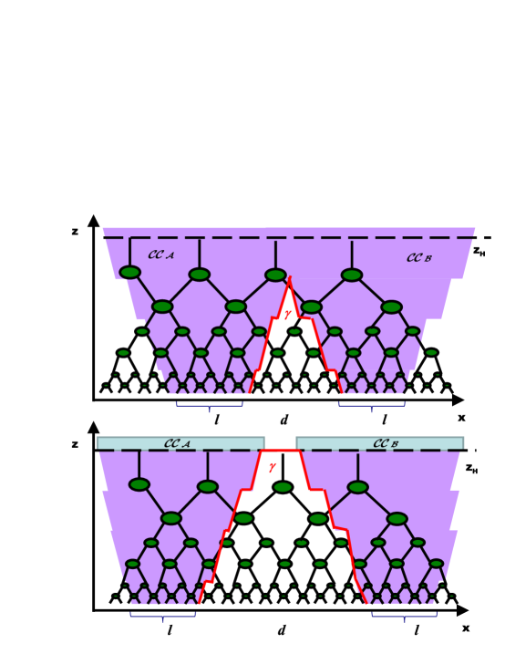
Figure 1: Top: Schematic representation of MERA ${\mathcal{CC}}$ for two disjoint finite intervals $A$ and $B$ when the separation between them allows for overlapping after $w_{*}\sim\log{\mathit{d}}$ renormalization steps. The overlap occurs before the causal cones shrink to one (in our representation, when causal cones stabilize their width after $w_{H}=\log{\it l}$ renormalization steps). Bottom: Schematic representation of MERA ${\mathcal{CC}}$ for two disjoint finite intervals $A$ and $B$ when the separation between them does not allow for overlapping after $w^{*}\sim\log{\mathit{d}}$ renormalization steps. The curve $\gamma$ that goes through the links between the nodes of the MERA network is the minimal curve separating the ${\mathcal{CC}}(A)$ and ${\mathcal{CC}}(B)$ from the traced out sites in the MERA bulk geometry (16).

3 The BTZ black hole

3.1 BTZ black hole solution

Bañados, Teitelboim, and Zanelli (BTZ) showed that (2+1)-dimensional gravity has a black hole solution, the BTZ black hole, differing from the Schwarzschild and Kerr solutions mainly in that it is asymptotically anti-de Sitter rather than asymptotically flat. The BTZ solution is clearly a black hole: it has an event horizon and (when rotating) an inner horizon, and it exhibits thermodynamic properties much like those of a (3+1)-dimensional black hole btz92 .

The BTZ black hole may be obtained by orbifolding $\rm{AdS}_{3}$ through $SL(2,{\mathbf{C}})$ identifications kraus06 and is a solution of pure gravity in three dimensions with a negative cosmological constant described by the Einstein-Hilbert action supplemented by boundary terms kraus06 ,

$$I=\frac{1}{16\pi G}\int\!d^{3}x\sqrt{g}\,(R-\frac{2}{\ell^{2}})+I_{\rm bndy}~{}.$$ (19)

In the following we use the Euclidean signature, and use the notation of Misner, Thorne, and Wheeler gravitation ; as a result, $r\equiv 1/z$ so that the boundary is now located at $r\to\infty$. A simple solution of the equations of motion is just the $\rm{AdS}_{3}$ spacetime,

$$ds^{2}=(1+r^{2}/\ell^{2})dt^{2}+\frac{dr^{2}}{1+r^{2}/\ell^{2}}+r^{2}d\phi^{2}~{}.$$ (20)

$\rm{AdS}_{3}$ has maximal symmetry, with the isometry group being $SL(2,{\mathbf{C}})\cong SL(2,{\mathbf{R}})_{L}\times SL(2,{\mathbf{R}})_{R}$.

A more general one-parameter family of solutions is provided by the non-rotating BTZ black hole of mass $M$ kraus06 ,

$$ds^{2}=\frac{(r^{2}-r_{+}^{2})}{\ell^{2}}dt^{2}+\frac{\ell^{2}}{(r^{2}-r_{+}^{2})}dr^{2}+r^{2}d\phi^{2}~{},$$ (21)

describing an $\rm{AdS}$ black hole with an event horizon located at $r=r_{+}=\ell\sqrt{8GM}$ at a temperature $T=r_{+}/2\pi\ell^{2}$; of course, for large $r$, the solution (21) asymptotically approaches $\rm{AdS}_{3}$.

The metric of a rotating BTZ black hole of mass $M$ and angular momentum $J$ is given, instead, by

$$ds^{2}=\frac{(r^{2}-r_{+}^{2})(r^{2}-r_{-}^{2})}{r^{2}\ell^{2}}dt^{2}+\frac{\ell^{2}r^{2}}{(r^{2}-r_{+}^{2})(r^{2}-r_{-}^{2})}dr^{2}+r^{2}(d\phi+i\frac{r_{+}r_{-}}{\ell r^{2}}dt)^{2}~{}.$$ (22)

with

$$M=\frac{r_{+}^{2}+r_{-}^{2}}{\ell^{2}}~{},\quad J=\frac{2r_{+}r_{-}}{\ell}~{},$$ (23)

$$r_{\pm}=\ell\left[\frac{M}{2}\left(1\pm\sqrt{1-\left(\frac{J}{M\ell}\right)^{2}}\right)\right]^{\frac{1}{2}}~{}.$$ (24)

Now, the event horizon is located at $r=r_{+}$ with $r_{+}\geq r_{-}$ and $r_{-}$ being the inner Cauchy horizon. Rotating BTZ black holes have been recently shown to be relevant in investigations of helical Tomonaga-Luttinger liquids Balasu2010 .

3.2 Dual CFT to the BTZ solution

The boundary of asymptotically $\rm{AdS}_{3}$ spacetimes is a two dimensional torus on which one can define a dual CFT with its conformal symmetry being generated by two copies of the Virasoro algebra acting separately on the left and right moving sectors. As a result, the CFT splits into two independent sectors at thermal equilibrium with temperatures,

$$T_{L}=\frac{r_{+}+r_{-}}{2\pi\ell^{2}}~{},\quad T_{R}=\frac{r_{+}-r_{-}}{2\pi\ell^{2}}~{}.$$ (25)

The mass $M$ and the angular momentum $J$ in the rotating BTZ black hole geometry are related to the Virasoro charges of the dual CFT on the boundary by

$$L_{0}-\frac{c}{24}=\frac{1}{16G}(M\ell+J)~{},\quad\widetilde{L}_{0}-\frac{\widetilde{c}}{24}=\frac{1}{16G}(M\ell-J)~{}.$$ (26)

with $c=\widetilde{c}$ given by the Brown-Henneaux holographic relation brownhenn

$$c=\frac{3\ell}{2G_{N}^{(3)}}~{}.$$ (27)

In the non rotating BTZ metric (21) one has

$$L_{0}-\frac{c}{24}=\widetilde{L}_{0}-\frac{\widetilde{c}}{24}=\frac{r_{+}^{2}}{16G\ell}~{}.$$ (28)

It is easy to prove kraus06 that, for the AdS₃ metric, (20) $L_{0}=\widetilde{L}_{0}=0$; this is just a consequence of its invariance under the $SL(2,\mathbf{R})_{L}\times SL(2,\mathbf{R})_{R}$ group of isometries generated by $L_{0,\pm 1}$ and $\widetilde{L}_{0,\pm 1}$.

3.3 Geodesics in the BTZ geometry

The RT formula uses the spacelike geodesics in a given metric. For the BTZ black hole these geodesics are well known. The length of the geodesics connecting two points $x_{i}$ and $x_{j}$ separated by a distance $|x_{i}-x_{j}|$ and located at the boundary of the AdS₃ space whose metric is described by a BTZ Black Hole (21), can be written as Ross00 ,

$$\mathit{L}(x_{i},x_{j})=2\ell\log\left[\frac{\beta}{\pi\epsilon}\sinh\left(\frac{\pi|x_{i}-x_{j}|}{\beta}\right)\right]~{},$$ (29)

with $\beta=2\pi\ell^{2}/r_{+}$ and $\epsilon$ the regularizing boundary cut-off.

Using the RT formula (5) and (27), one gets the well known formula Calabrese04 for the EE of a single connected block $A$ of length $\ell_{A}=|x_{1}-x_{2}|$ from the BTZ geometry; namely, one has that

$$S_{A}=\frac{\mathit{L}(x_{1},x_{2})}{4G_{N}^{(3)}}=\frac{c}{3}\log\left[\frac{\beta}{\pi\epsilon}\sinh\left(\frac{\pi\ell_{A}}{\beta}\right)\right]$$

$$\approx\begin{cases}(c/3)\log\left(\ell_{A}/\epsilon\right)\,,\quad&r_{+}\to 0\ (\beta\to\infty)\\ \\ (\pi c/3)(\ell_{A}/\beta)+\frac{c}{3}\log(\beta/2\pi\epsilon)\,,\quad&r_{+}\to\infty\ (\beta\to 0)\end{cases}\,.$$ (30)

As expected, from eq. (3.3) one recovers the logarithmic dependence only in the zero temperature limit (i.e., when the size of the interval is small in comparison with the distance of the horizon from the boundary); indeed, in this limit, the BTZ geodesics stay close to the boundary and only probe the asymptotic form of the ${\rm AdS}_{3}$ BTZ geometry. (Fig.2 Left). At variance, when the size of the simply connected region $A$ is bigger than the distance of the horizon from the boundary, the BTZ geodesics probe the black hole horizon extending tangentially to it; this induces the linear correction to the EE which, for a single connected region $A$, describes now a thermal state at temperature $T=1/\beta$ (Fig.2 Right).

For a rotating black hole, the geodesics are given instead by

$$\mathit{L}(x_{i},x_{j})=2\ell\log\left[\frac{\beta_{L}\beta_{R}}{\pi^{2}\epsilon^{2}}\sinh\left(\frac{\pi|x_{i}-x_{j}|}{\beta_{L}}\right)\sinh\left(\frac{\pi|x_{i}-x_{j}|}{\beta_{R}}\right)\right]~{},$$ (31)

where $\beta_{L,R}=1/T_{L,R}$. As a result one gets that

$$S_{A}=S_{A}^{L}+S_{A}^{R}=$$

$$=\frac{c}{3}\log\left[\frac{\beta_{L}}{\pi\epsilon}\sinh\left(\frac{\pi\ell_{A}}{\beta_{L}}\right)\right]+\frac{c}{3}\log\left[\frac{\beta_{R}}{\pi\epsilon}\sinh\left(\frac{\pi\ell_{A}}{\beta_{R}}\right)\right]~{}.$$ (32)

Equation (32) factorizes into left and right moving sectors as expected from the left-right decoupling of the CFT₂.

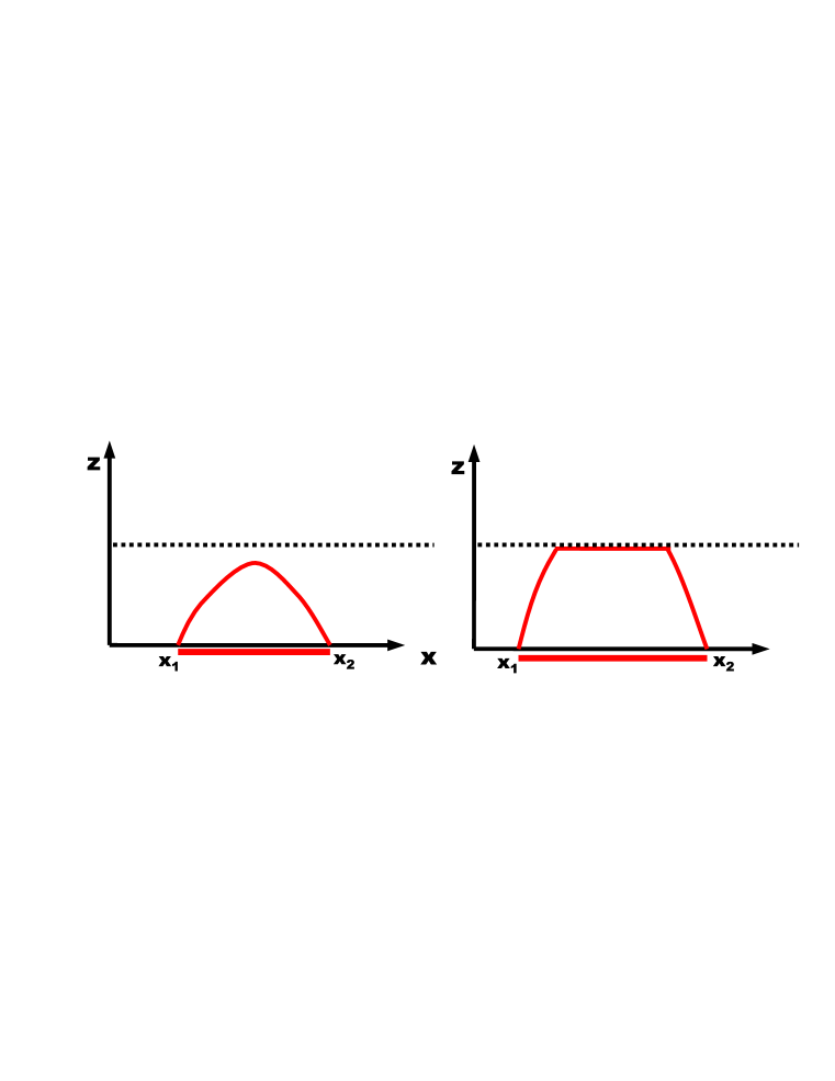
Figure 2: Geodesic used in computing the entanglement entropy of a region of length ${\mathit{l}}=|x_{1}-x_{2}|$ in the AdS Black Hole geometry. Left: $\gamma$ does not approach the horizon (dotted line). Right: $\gamma$ wraps around the horizon.

4 Holographic Computation of Quantum Correlations and Mutual Information for two disjoint intervals

In this section we derive both the MI and the quantum correlations between two disjoint intervals of a one dimensional critical system described by a CFT₂ located at the boundary of the AdS₃ space. We assume in the following that the disjoint intervals $A$ and $B$ have equal size ${\mathit{l}}$ and are separated by a distance ${\mathit{d}}$. Namely, we take $A\equiv\left[u_{1},v_{1}\right],B\equiv\left[u_{2},v_{2}\right]$ with $|u_{1}-v_{1}|=|u_{2}-v_{2}|={\mathit{l}}$ and $|v_{1}-u_{2}|={\mathit{d}}$ (see Fig.3). We shall see how, in both computations, one can find a critical value of a pertinent parameter at which there is a transition between two very different behaviors.

For the two disjoint intervals $A$ and $B$ the holographic computation of the MI requires to determine the minimal curve in the bulk homologous to $A\cup B$. In the MERA induced AdS/CFT correspondence, the curve $\gamma_{A\cup B}$ is generated by tracing out the bulk sites lying outside the ${\mathcal{CC}}(A)$ and ${\mathcal{CC}}(B)$ and is an holographic screen for the entropy contained in $A\cup B$. As a result, for generating this holographic screen, there are- just as in headrick10 - only two possible options given by $\gamma_{A\cup B}^{(con)}$ (Fig 3 Left) and $\gamma_{A\cup B}^{(dis)}$ (Fig 3 Right), respectively: the curve $\gamma_{A\cup B}^{(con)}$ ($\gamma_{A\cup B}^{(dis)}$) corresponds to the overlapping (non-overlapping) configuration of the causal cones ${\mathcal{CC}}(A)$ and ${\mathcal{CC}}(B)$ depicted in Fig 1. Namely, $\gamma^{(dis)}_{A\cup B}$, describes a situation in which the two intervals are enough separated so that ${\mathit{L}}_{A\cup B}={\mathit{L}}_{1}(u_{1},v_{1})+{\mathit{L}}_{2}(u_{2},v_{2})$, while $\gamma^{(con)}_{A\cup B}$, describes a situation where the separation between the intervals is so small that the minimal curve of the region $A\cup B$, connects the inner and outer boundaries of the two regions so that ${\mathit{L}}_{A\cup B}={\mathit{L}}_{1}(u_{1},v_{2})+{\mathit{L}}_{2}(v_{1},u_{2})$.

Of course, when $\gamma^{(dis)}_{A\cup B}$ is used in the holographic computation of the MI, the MI vanishes as a consequence of eqs. (5) and (18). At variance, when one uses $\gamma_{A\cup B}^{(con)}$, the holographic computation of the MI (18), using as the metric of the AdS₃ bulk space the one corresponding to a BTZ black hole with the horizon located at $z_{+}={\mathit{l}}$ from the boundary i.e $\beta=2\pi z_{+}$, yields (27)

$$I_{(A:B)}=\frac{c}{3}\log\left[\frac{\sinh\left(\pi T|u_{1}-v_{1}|\right)\,\sinh\left(\pi T|u_{2}-v_{2}|\right)}{\sinh\left(\pi T|u_{1}-v_{2}|\right)\,\sinh\left(\pi T|v_{1}-u_{2}|\right)}\right]~{},$$ (33)

with $T=1/\beta$.

One sees that $I_{(A:B)}$ in eq. (33) equals zero when a certain ratio between ${\mathit{l}}=|u_{1}-v_{1}|=|u_{2}-v_{2}|$ and ${\mathit{d}=|v_{1}-u_{2}|}$ is reached; namely, one sees that the MI, when computed using the BTZ black hole as the metric of AdS₃, vanishes at a value of the conformal four point ratio given by $x_{0}\sim 0.53$. This is in agreement with the result of headrick10 . However, an advantage of the MERA induced AdS/CFT correspondence lies in the fact that one can provide a rather intuitive entropic argument accounting for the use of either one of the two minimal curves depicted in Fig.3 when performing the holographic computation of MI. Indeed, since the length of the curves $\gamma_{A\cup B}^{(con)}$ and $\gamma_{A\cup B}^{(dis)}$ are- by definition- the sum of the entropies of all the traced out sites, the transition between the two behaviors of MI occurs when the separation between the two (equal size) disjoint blocks $A$ and $B$ is such that the entropy due to the the tracing out process yielding $\gamma_{A\cup B}^{(con)}$ equals the entropy due to the tracing out process yielding $\gamma_{A\cup B}^{(dis)}$.

A similar transition is found also in the computation of the quantum correlations between two primary operators ${\cal O}(x_{A})$ and ${\cal O}(x_{B})$ ($x_{A}\in A$ and $x_{B}\in B$) with conformal dimension $\Delta$ defined in the CFT${}_{d}+1$ describing the boundary critical system. This should be expected in view of the bound (11). The $\rm{AdS}/\rm{CFT}$ correspondence implies AdSCFTbible00 ; Witten98 that

$$\langle{\cal O}(x_{A}){\cal O}(x_{B})\rangle\sim e^{-m{\mathit{L}}(x_{A},x_{B})}~{},$$ (34)

where $\Delta\approx m\ell$ and ${\mathit{L}}(x_{A},x_{B})$ is the length of the shortest geodesic connecting the boundary points $x_{A}$ and $x_{B}$. Using for ${\mathit{L}}(x_{A},x_{B})$ the expression given in (29), one easily gets,

$$\langle{\cal O}(x_{A}){\cal O}(x_{B})\rangle\sim\left[\frac{\pi T}{\sinh\left(\pi T|x_{A}-x_{B}|\right)}\right]^{2\Delta}$$

$$\approx\begin{cases}|x_{A}-x_{B}|^{-2\Delta}\,,\quad&z_{+}\gg|x_{A}-x_{B}|\\ \\ z_{+}^{-2\Delta}\exp\left(-2\pi T\Delta|x_{A}-x_{B}|\right)\,,\quad&z_{+}\ll|x_{A}-x_{B}|\end{cases}\,.$$ (35)

From (35) one sees that there is a change from an algebraic to an exponential decaying behavior of the two point quantum correlation function and that the transition between the two regimes occurs when $\langle{\cal O}(x_{A}){\cal O}(x_{B})\rangle\sim e^{-\Delta}$. When this happens, one has that

$$2\pi\,T\,|x_{A}-x_{B}|=\frac{|x_{A}-x_{B}|}{z_{+}}\approx 1~{},$$ (36)

which defines the value of the parameter $\mu=|x_{A}-x_{B}|/{\mathit{l}}$ at which this transition occurs tonni10 .

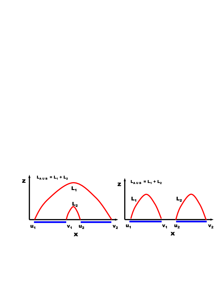
Figure 3: Minimal curves used in the holographic computation of $S_{A\cup B}$ and $I_{(A:B)}$ for to disjoint intervals $A$ and $B$.

Eqs. (33) and (35) are derived for infinite systems when the central charge $c\to\infty$. However, one may be interested in the behavior of the MI and of the quantum correlations in a regime where both the temperature $T$ and the size of the system $L$ are finite Birmingham2002 . In particular, one is interested in knowing if the transition between the two very distinct behaviors found for the infinite system is still attainable and, if so, how the critical value of the pertinent parameter is going to be affected when $T$ and $L$ are finite. To grasp how the results obtained so far in this section are going to be changed due to these finite size effects we look at the behavior of the two point correlation functions of free fermions on the torus Francesco97 . For this system one has that,

$$\langle\psi(u)\psi(v)\rangle_{\nu}=\frac{\theta_{\nu}(i|u-v|T\,|\tau)}{\theta_{\nu}(0|\tau)}\,\frac{\partial_{\omega}\theta_{1}(0|\tau)}{\theta_{1}(i|u-v|T\,|\tau)}~{},$$ (37)

where $\theta_{\nu}(\omega|\tau)$ are the modular Jacobi theta functions tatatheta , $\partial_{\omega}\theta_{1}(0|\tau)\equiv\partial_{\omega}\theta_{1}(\omega|\tau)|_{\omega=0}$, $\nu$ defines the boundary conditions for $\psi$ and $\tau\equiv iLT$. For instance, for finite temperature boundary conditions, only the sectors $\nu=3,4$ of the spin structure of the fermion contribute (37); this is to say that, on the torus, one can only choose for $\psi$ either $\nu=3$, corresponding to antiperiodic-periodic (Neveu-Schwarz, NS - Ramond, R) boundary conditions, or $\nu=4$ which corresponds to antiperiodic-antiperiodic (NS-NS) boundary conditions.

When $LT\to\infty$, using the standard representation of the $\theta_{\nu}$ functions tatatheta ; Alvarez86 , one gets

$$\langle\psi(u)\psi(v)\rangle_{3(4)}=\frac{\pi T}{4\sinh{\pi T|u-v|}}[1\pm 2e^{-\pi LT}\cosh 2\pi T|u-v|+...]~{},$$ (38)

As a result, in the limit of finite $T$ with $L\gg|u-v|$, one may approximate Eq. (35) with $\Delta=1/2$ in terms of (37) and write (33) as,

$$I_{(A:B)}=\frac{c}{3}\left[\frac{\Upsilon(v_{2},u_{1})\,\Upsilon(u_{2},v_{1})}{\Upsilon(v_{1},u_{1})\,\Upsilon(v_{2},u_{2})}\right]+\frac{c}{3}\log\left[\frac{\theta_{\nu}(i|u_{1}-v_{2}|T\,|\tau)\,\theta_{\nu}(i|u_{2}-v_{1}|T\,|\tau)}{\theta_{\nu}(i|u_{1}-v_{1}|T\,|\tau)\,\theta_{\nu}(i|u_{2}-v_{2}|T\,|\tau)}\right]~{},$$ (39)

where $\Upsilon(u,v)$ is given by Francesco97

$$\Upsilon(u,v)=\log\frac{\partial_{\omega}\theta_{1}(0|\tau)}{\theta_{1}(i|u-v|T\,|\tau)}~{}.$$ (40)

For $L\gg|u-v|$ one has that $\Upsilon(u,v)\sim\log 1/(i|u-v|T)$; as a result one has

$$I_{(A:B)}=\frac{c}{3}\log\left(\frac{x}{1-x}\right)+\frac{c}{3}\log\left[\frac{\theta_{\nu}(i|u_{1}-v_{2}|T\,|\tau)\,\theta_{\nu}(i|u_{2}-v_{1}|T\,|\tau)}{\theta_{\nu}(i|u_{1}-v_{1}|T\,|\tau)\,\theta_{\nu}(i|u_{2}-v_{2}|T\,|\tau)}\right]~{},$$ (41)

where $x$ is defined in (13). One notices that (41) reduces to (14) when the separation between the intervals is very small since the function $f_{\nu}(x,\tau)$ defined as

$$f_{\nu}(x,\tau)=\log\left(\frac{\theta_{\nu}(i|u_{1}-v_{2}|T\,|\tau)\,\theta_{\nu}(i|u_{2}-v_{1}|T\,|\tau)}{\theta_{\nu}(i|u_{1}-v_{1}|T\,|\tau)\,\theta_{\nu}(i|u_{2}-v_{2}|T\,|\tau)}\right)~{},$$ (42)

approaches zero when $x\to 1$ while $f_{\nu}(x,\tau)>0$ for $x\leq 1$.

We observe that, in a rather large range of values for $T$ and $L$, there is still a transition between two very different behaviors of the MI. However, the critical value $x_{0}$, at which the transition occurs strongly depends on the ratio ${\mathit{l}}/L$ i.e, $1/|\tau|=(LT)^{-1}$ as reported in Fig. 4. Indeed, a numerical analysis shows that, for a finite system, $x_{0}$ is always $x_{0}<1/2$ and that, only as $L\to\infty$, $x_{0}\to 1/2$ recovering the result in headrick10 .

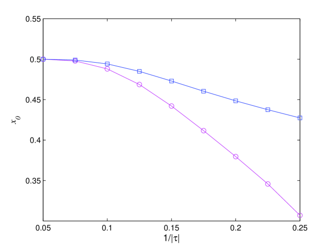
Figure 4: Dependence of the transition point $x_{0}$ on $|\tau|=LT$ i.e $1/|\tau|\propto{\mathit{l}}/L$ for the non rotating BTZ black hole (Eq (41), circles) and for the quasi-extremal rotating BTZ black hole (Eq (45), squares).

For the sake of completeness we shall compute the quantum correlators and the MI in a rotating BTZ black hole background in Appendix A.

5 Concluding Remarks

Originally developed within string theory, the AdS/CFT correspondence provides a geometrical framework to investigate also strongly coupled condensed matter and spin systems at criticality . An intriguing observation has been that MERA Vidal07 may be efficiently described through the AdS/CFT correspondence by introducing an AdS metric in a pertinently engineered bulk space swingle09 ; Evenbly11 . In this paper we use this MERA induced AdS/CFT correspondence to provide a framework in which the mutual information and the two point quantum correlations between disjoint blocks of a quantum system at criticality may be evaluated. We feel that an advantage of this approach is that, at least in principle, is not strictly confined to the analysis of one dimensional critical systems.

In order to get an hint on the pertinent metric to be used to describe the MERA induced bulk AdS_d+2 space, we observed here that, when computing the quantum correlations between two disjoint blocks of a boundary quantum critical system, the structure of the causal cones characteristic of MERA implies the existence of two different regimes attainable by tuning the ratio between the size and the separation of the disjoint blocks. To account for this transition we proposed that the MERA induced holographic dual bulk spacetime could be described by an AdS_d+2 black hole and used the RT formula to compute the MI of two disjoint regions of the boundary critical system. Intuitively speaking, this amounts to orbifolding the AdS geometry introduced in swingle09 ; Evenbly11 when dealing with disjoint blocks.

As an explicit example, we used a BTZ $\rm{AdS}_{3}$ black hole to compute the MI and the quantum correlations between two disjoint intervals of a one dimensional boundary quantum critical system: here, our analysis not only confirmed the existence of the phase transition emerging when the conformal four point ratio reaches a critical value but also provided a rather intuitive entropic argument explaining the source of this instability. Furthermore, we showed how non universal behaviors may emerge in the holographic computation of the MI between two well separated disjoint blocks. Of course, our analysis does not exclude the possibility that other geometries -such as Lifshitz geometries- may account for the behavior of the causal cones of disjoint blocks in MERA.

A remarkable feature of the RT approach to the computation of MI and EE taken in this paper is that it associates with each spatial region of the boundary a unique spatial region of the bulk Fursaev06 . This bulk to boundary map -via the structure of the causal cones- seems to play an intriguing role also in MERA. Indeed, we exploited this map in MERA to give an ansatz for the dual holographic geometry associated to a region made of two disjoint blocks of the $d$-dimensional boundary critical system. We, then, observed that -when the separation between the two blocks exceeds a critical value- the quantum correlations exhibit a thermal behaviour and the EE may be computed as the thermodynamic entropy associated to a certain black hole. In the context of the AdS/CFT correspondence thermal states have been recently constructed in CasHuMyers2011 .

The AdS/CFT correspondence, is a strong-weak duality. This amounts to say that, when the dual gravity description of a quantum system is classical, the correlations on the boundary theory are quantum and highly non-local (entanglement) VanRaamsdonk2009 . In the MERA induced AdS/CFT correspondence, the locality of the emerging AdS space is due to the existence of entanglement at all scales in the quantum critical system located at the boundary. We feel that our results may help to elucidate the nature (quantum and/or classical) of the correlations computed using the RT formula within the AdS/CFT correspondence. Indeed, despite the fact that MI quantifies both classical and quantum correlations, recently, in headrick11 , it has been shown that MI, when computed using the holographic RT formula, obeys the same monogamy relations required for a true measure of entanglement. Since the monogamy relations severely limit the amount of entanglement sharable between the different parts of an arbitrarily partitioned system coffman00 this should imply a truly quantum nature of the correlations measured in the holographic computation of the MI. In Wichterich09_2 , using numerical methods to compute a true measure of entanglement such as negativity, it has been found that the entanglement between disjoint intervals in spin chains at criticality also showed a crossover from pure algebraic decay to pure exponential decay when a critical ratio between the separation and the size of the intervals was reached.

Finally, we feel that the use of a pertinent metric in the AdS space built from the MERA induced AdS/CFT correspondence may be exploited also as a way to look for alternative and- hopefully- more powerful ways of optimizing MERA tensor networks.

Appendix A Quantum correlators and MI in the rotating BTZ background

In this appendix we compute the MI and quantum correlations between two disjoint intervals of the same size ${\mathit{l}}$ when the background metric is a rotating BTZ black hole.

When the distance between the two intervals is small enough, the geodesic of minimal length is ${\mathit{L}}_{A\cup B}^{(con)}={\mathit{L}}(u_{1},v_{2})+{\mathit{L}}(v_{1},u_{2})$; using (31), one gets

$$I_{(A:B)}=\frac{c}{3}\log\left[\frac{\sinh^{2}\left(\pi T_{L}\varrho_{1}\right)}{\sinh\left(\pi T_{L}\varrho_{2}\right)\sinh\left(\pi T_{L}\varrho_{3}\right)}\frac{\sinh^{2}\left(\pi T_{R}\varrho_{1}\right)}{\sinh\left(\pi T_{R}\varrho_{2}\right)\sinh\left(\pi T_{R}\varrho_{3}\right)}\right]~{},$$ (43)

where $\varrho_{1}\equiv|u_{1}-v_{1}|=|u_{2}-v_{2}|={\mathit{l}}$, $\varrho_{2}\equiv|u_{2}-v_{1}|={\mathit{d}}$ and $\varrho_{3}\equiv|u_{1}-v_{2}|=2{\mathit{l}}+{\mathit{d}}$. In equation (43), the event horizon is located at $z_{+}=1/r_{+}={\mathit{l}}$ and, upon introducing the two variables $z_{L}=1/(r_{+}+r_{-})$ and $z_{R}=1/(r_{+}-r_{-})$ such that $z_{L}<z_{+}<z_{R}$, one is able to define the two temperatures $T_{L}=1/2\pi z_{L}$ and $T_{R}=1/2\pi z_{R}$ (Fig.5).

For the near extremal BTZ black hole, i.e, for a black hole in which $M\ell\gtrsim J$ ($r_{+}\gtrsim r_{-}$, $z_{R}\to\infty$), equation (43) may be written as,

$$I_{(A:B)}=\frac{c}{3}\log\left(\frac{x}{1-x}\right)+\frac{c}{3}\log\left[\frac{\sinh^{2}\left(\pi T_{L}\varrho_{1}\right)}{\sinh\left(\pi T_{L}(\pi T_{L}\varrho_{2}\right)\sinh\left(\pi T_{L}\varrho_{3}\right)}\right]~{}.$$ (44)

One sees from equation (44) that the decoupling of the right and left moving sectors induced by the presence of two horizons, plus the near extremality condition of the spinning black hole, yields an expression for the MI which decomposes in two terms: one -identical to (14)-depends only on $c$ and the conformal ratio $x$- and a second identical to (33). It is easy to convince oneself that equation (41) when $T=T_{L}$ reproduces the second term of (44). As a result, the MI of two disjoint intervals in a finite system of total length $L$ may be written as,

$$I_{(A:B)}=\frac{2c}{3}\log\left(\frac{x}{1-x}\right)+\frac{c}{3}\log\left(\frac{\theta_{\nu}(i|u_{1}-v_{2}|T_{L}\,|\tau)\,\theta_{\nu}(i|u_{2}-v_{1}|T_{L}\,|\tau)}{\theta_{\nu}(i|u_{1}-v_{1}|T_{L}\,|\tau)\,\theta_{\nu}(i|u_{2}-v_{2}|T_{L}\,|\tau)}\right)~{},$$ (45)

with $\tau=iLT_{L}$.

For the rotating extremal BTZ black hole, numerical simulations show that $1/|\tau|$ weakly affects the location of the transition point $x_{0}$ for the MI (Fig. 4). Furthermore, it appears from our results and those presented in headrick10 , that the MI is parametrically small at $x_{0}$. As a result, due to the inequality (11), one should expect also here a transition for the quantum correlations.

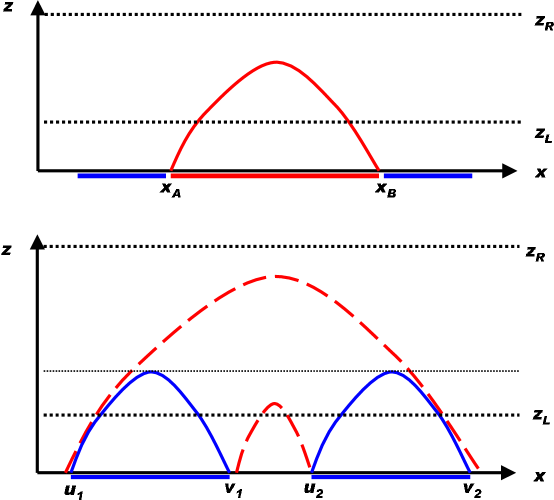
Figure 5: Characteristic length scales $z_{R}$ and $z_{L}$ of the rotating BTZ black hole background. The event horizon $z_{+}$ lies between $z_{L}<z_{+}<z_{R}$ (thin dotted line between $z_{L}$ and $z_{R}$). Top. Geodesic connecting the two closest boundary points of the intervals $A$ and $B$ used in the computation of eq. (46). Bottom: Geodesic ${\mathit{L}}_{A\cup B}^{(con)}={\mathit{L}}(u_{2},v_{2})+{\mathit{L}}(v_{1},u_{2})$ used in the computation of eq. (44).

For the rotating BTZ black hole, the behavior of the quantum correlations between points located in different disjoint intervals is given by,

$$\langle{\cal O}(x_{A}){\cal O}(x_{B})\rangle\sim\left[\frac{\beta_{L}\beta_{R}}{\pi^{2}}\sinh\left(\frac{\pi|x_{A}-x_{B}|}{\beta_{L}}\right)\sinh\left(\frac{\pi|x_{A}-x_{B}|}{\beta_{R}}\right)\right]^{-2\Delta}~{}.$$ (46)

When the near extremality condition is satisfied, ${\it i.e}$, when $r_{+}\gtrsim r_{-}$, so $\beta_{R}\to\infty$, the two point correlations behave as,

$$\langle{\cal O}(x_{A}){\cal O}(x_{B})\rangle\sim\left(\frac{1}{|x_{A}-x_{B}|}\right)^{2\Delta}\left(\frac{2\pi}{\beta_{L}}\right)^{2\Delta}\exp\left(-\frac{2\pi\Delta|x_{A}-x_{B}|}{\beta_{L}}\right)~{}.$$ (47)

Eq. (47) shows the existence of a crossover from pure algebraic decay to pure exponential decay of the quantum correlations as $\mu=|x_{A}-x_{B}|/z_{+}$ increases.

- (1) C. Holzhey, F. Larsen, and F. Wilczek, Geometric and renormalized entropy in conformal field theory, Nucl. Phys. B 424 (1994), no. 3 443–467, [hep-th/9403108].
- (2) M. Caraglio and F. Gliozzi, Entanglement entropy and twist fields, JHEP 2008 (2008), no. 11 076, [arXiv:0808.4094].
- (3) P. Calabrese and J. Cardy, Entanglement entropy and quantum field theory, J. Stat. Mech.: Theory Exp. P06002 (2004) [hep-th/0405152].
- (4) S. Ryu and T. Takayanagi, Aspects of holographic entanglement entropy, JHEP 0608:045 (2006) [hep-th/0605073].
- (5) S. Ryu and T. Takayanagi, Holographic derivation of entanglement entropy from , Phys. Rev. Lett. 96 (2006) 181602, [hep-th/0603001].
- (6) D. V. Fursaev, Proof of the holographic formula for entanglement entropy, JHEP 9 (2006) 18–+, [hep-th/0606184].
- (7) H. Casini, M.Huerta, and R. C. Myers, Towards a derivation of holographic entanglement entropy, JHEP 036 (2011) 1105, [arXiv:1102.0440].
- (8) M. Headrick and T. Takayanagi, Holographic proof of the strong subadditivity of entanglement entropy, Phys. Rev. D 76 (2007), no. 10 106013, [arXiv:0704.3719].
- (9) O. Aharony, S. Gubser, J. Maldacena, H. Ooguri, and Y. Oz, Large field theories, string theory and gravity, Phys. Rep. 323 (2000) 183, [hep-th/9905111].
- (10) L. Susskind and E. Witten, The holographic bound in nti de itter space, hep-th/9805114.
- (11) S. Furukawa, V. Pasquier, and J. Shiraishi, Mutual information and boson radius in c=1 critical systems in one dimension, Phys. Rev. Lett. 102 (2009) 170602, [arXiv:0809.5113].
- (12) P. Calabrese, J. Cardy, and E. Tonni, Entanglement entropy of two disjoint intervals in conformal field theory, J. Stat. Mech.: Theory Exp. P11001 (2009) [arXiv:0905.2069].
- (13) M. W. Wolf, F. Verstraete, M. Hastings, and J. Cirac, Area laws in quantum systems: Mutual information and correlations, Phys Rev Lett 100 (2008) 070502, [arXiv:0704.3906].
- (14) G. Vidal and R. F. Werner, A computable measure of entanglement, Phys. Rev. A 65 (Feb, 2002) 032314, [quant-ph/0102117].
- (15) H. Wichterich, J. Molina-Vilaplana, and S. Bose, Scaling of entanglement between separated blocks in spin chains at criticality, Phys. Rev. A 80 (2009) 010304(R), [arXiv:0811.1285].
- (16) S. Marcovitch, A. Retzker, M. B. Plenio, and B. Reznik, Critical and noncritical long-range entanglement in Klein-Gordon fields, Phys. Rev. A 80 (2009) 012325, [arXiv:0811.1288].
- (17) H. Casini and M. Huerta, A finite entanglement entropy and the c-theorem, Phys. Lett. B600 (2004) 142–150, [hep-th/0405111].
- (18) H. Casini, C. Fosco, and M. Huerta, Entanglement and alpha entropies for a massive Dirac field in two dimensions, J. Stat. Mech. 0507 (2005) P007, [cond-mat/0505563].
- (19) M. Headrick, Entanglement Rényi entropies in holographic theories, Phys. Rev D 82 (2010), no. 12 126010, [arXiv:1006.0047].
- (20) B.-Q. Jin and V. Korepin, Entanglement entropy for disjoint subsystems in XX spin chain, arXiv:1104.1004.
- (21) S. Hawking and D. Page, Thermodynamics of black holes in nti-de itter space, Commun. Math. Phys. 87 (1982) 577–588.
- (22) B. Swingle, Entanglement renormalization and holography, arXiv:0905.1317.
- (23) B. Swingle, Mutual information and the structure of entanglement in quantum field theory, arXiv:1010.4038.
- (24) G. Evenbly and G. Vidal, Tensor network states and geometry, arXiv:1106.1082.
- (25) G. Vidal, Class of quantum many-body states that can be efficiently simulated, Physical Review Letters 101 (2008), no. 11 110501, [quant-ph/0610099].
- (26) G. Vidal, Entanglement renormalization, Phys. Rev. Lett. 99 (2007) 220405, [cond-mat/0512165v2].
- (27) D. J. Gross and H. Ooguri, Aspects of large gauge theory dynamics as seen by string theory, Phys. Rev. D 58 (1998) 106002, [hep-th/9805129].
- (28) M. V. Raamsdonk, Comments on quantum gravity and entanglement, arXiv:0907.2939.
- (29) J. Haegeman, T. J. Osborne, H. Verschelde, and F. Verstraete, Entanglement renormalization for quantum fields, arXiv:1102.5524.
- (30) M. Bañados, C. Teitelboim, and J. Zanelli, Black hole in three-dimensional spacetime, Phys. Rev. Lett. 69 (Sep, 1992) 1849–1851, [hep-th/9204099].
- (31) P. Kraus, Lectures on black holes and the correspondence, LectNotesPhys 755 (2008) 193–247, [hep-th/0609074].
- (32) C. Misner, K. Thorne, and J. Wheeler, Gravitation. W. H. Freeman, 1973.
- (33) V. Balasubramanian, I. García-Etxebarria, F. Larsen, and J. Simón, Helical uttinger liquids and three dimensional black holes, arXiv:1012.4363.
- (34) J. D. Brown and M. Henneaux, Central charges in the canonical realization of asymptotic symmetries: An example from three dimensional gravity, Communications in Mathematical Physics 104 (1986) 207–226. 10.1007/BF01211590.
- (35) J. Louko, D. Marolf, and S. F. Ross, On geodesic propagators and black hole holography, Phys. Rev. D 62 (2000) 044041, [hep-th/0002111].
- (36) E. Witten, Anti de sitter space and holography, Adv.Theor.Math.Phys. 2 (1998) 253–291.
- (37) E. Tonni, Holographic entanglement entropy: near horizon geometry and disconnected regions, arXiv:1011.0166.
- (38) D. Birmingham, I. Sachs, and S. Solodukhin, Relaxation in conformal field theory, awking-age transition, and quasinormal/normal modes, Phys. Rev. D 67 (2003) 104026, [hep-th/0212308].
- (39) P. D. Francesco, P. Mathieu, and D. Sénéchal, Conformal Field Theory. Springer, New York, 1997.
- (40) D. Mumford, TATA Lectures on Theta. Birkhauser, 1982.
- (41) L. Alvarez-Gaumé, G. Moore, and C. Vafa, Theta functions, modular invariance, and strings, Communications in Mathematical Physics 106 (1986) 1–40.
- (42) P. Hayden, M. Headrick, and A. Maloney, Holographic mutual information is monogamous, arXiv:1107.2940.
- (43) V. Coffman, J. Kundu, and W. Wootters, Distributed entanglement, Phys. Rev. A 61 (Apr, 2000) 052306, [quant-ph/9907047].