Critical exponents from two-particle irreducible 1/$N$ expansion

Abstract

We calculate the critical exponent $\nu$ in the $1/N$ expansion of the two-particle-irreducible (2PI) effective action for the $O(N)$ symmetric $\varphi^{4}$ model in three spatial dimensions. The exponent $\nu$ controls the behavior of a two-point function $\langle\varphi\varphi\rangle$ near the critical point $T\neq T_{c}$, but can be evaluated on the critical point $T=T_{c}$ by the use of the vertex function $\Gamma^{(2,1)}$. We derive a self-consistent equation for $\Gamma^{(2,1)}$ within the 2PI effective action, and solve it by iteration in the $1/N$ expansion. At the next-to-leading order in the $1/N$ expansion, our result turns out to improve those obtained in the standard one-particle-irreducible calculation.

I Introduction

Understanding equilibrium and nonequilibrium phenomena associated with phase transitions has become more and more important in various fields in physics, such as early-time universe, ultra-relativistic heavy-ion collisions, ultra-cold atoms, and so on CalHu ; Boyanovsky:2006bf . In a second-order phase transition, characteristic long-range fluctuations appear in the order parameter field, and for a quantitative study of static and dynamic critical phenomena Hohenberg ; Mazenko , one needs a field theoretical method which can describe both static and dynamical processes involving strong fluctuations. Emergence of long-range fluctuations makes naive perturbation theory break down and requires some sort of resummation, such as the method of the renormalization group or the two-particle-irreducible (2PI) effective action LW ; CJT .

Recently, the method of the 2PI effective action has received much attention since it can be applied to the phenomena in and out of equilibrium on an equal footing Berges ; ABC ; JSD . In this method, all the self-energy contributions for the two-point correlation function are first summed up and then the perturbative expansion is carried out in terms of the full two-point correlation function. This is in contrast to the standard method of the one-particle-irreducible (1PI) effective action in which the perturbative expansion of the diagrams is done in terms of the free two-point correlation function. The method of the 2PI effective action systematically resums higher order terms in powers of coupling constants, so that it is expected to take into account efficiently the large fluctuations near the critical point.

In the present paper we restrict ourselves to static critical phenomena and leave dynamic critical phenomena for future study. As is well known, the most prominent feature of static critical phenomena is universality. In other words, several critical exponents which characterize the singularities in the vicinity of the critical point are solely determined by symmetry of the system, irrespective of microscopic details. In fact, only two of them are independent, and we take $\eta$ and $\nu$ to be studied in this paper. They can be read off from the two-point correlation function $G({\boldsymbol{x}},{\boldsymbol{0}})=\langle\varphi({\boldsymbol{x}})\varphi({\boldsymbol{0}})\rangle$ of the order parameter field as

$$G({\boldsymbol{x}},{\boldsymbol{0}})\sim\frac{1}{|{\boldsymbol{x}}|^{d-2+\eta}}\qquad(T=T_{c})\,,$$ (1)

$$G({\boldsymbol{x}},{\boldsymbol{0}})\sim{\rm e}^{-|{\boldsymbol{x}}|/\xi}\,,\quad\xi\sim|T-T_{c}|^{-\nu}\qquad(T>T_{c})\,,$$ (2)

where $d$ is the number of space dimensions (now $d=3$), $\xi$ is the correlation length, and $T_{c}$ is the critical temperature. Namely, $\eta$ and $\nu$ govern the behavior of two-point functions on and off the critical point, respectively. In the momentum space, the Fourier transform of Eq. $(\ref{eq:eta-x})$ gives the scaling form $\widetilde{G}({\boldsymbol{k}})\sim{|{\boldsymbol{k}}|^{\eta-2}}$.

Recently, Alford, Berges, and Cheyne employed the $1/N$ expansion of the 2PI effective action to compute the exponent $\eta$ of an $O(N)$-symmetric $\varphi^{4}$ theory in three dimensions ABC . They solved the 2PI Schwinger-Dyson equation (Kadanoff-Baym equation) KB paper ; Baym ; KB text at the critical point, substituting the scaling form to $\widetilde{G}({\boldsymbol{k}})$. It was shown that at the next-to-leading order (NLO) in the $1/N$ expansion this approach remedies the spurious divergence of $\eta$ at small $N$, which is seen in the 1PI $1/N$ expansion, and leads to an improved estimate already for moderate values of $N$. This success strongly motivated us to compute another exponent $\nu$ within the 2PI effective action. The exponent $\nu$ is also associated with the critical behavior of the two-point functions.

It is not straightforward, however, to apply this method to the evaluation of $\nu$. Given two nonzero parameters, $p$ and $T-T_{c}$, one needs to fix the form of $\widetilde{G}({\boldsymbol{p}};T)$ in the scaling region, which introduces a technical complication to the problem. Fortunately, we notice that the exponent $\nu$ can be determined from the three-point vertex function $\Gamma^{(2,1)}({\boldsymbol{x}},{\boldsymbol{y}};{\boldsymbol{z}})\sim\langle\varphi({\boldsymbol{x}})\varphi({\boldsymbol{y}})\varphi^{2}({\boldsymbol{z}})\rangle$ with two elementary fields, $\varphi$, and one composite operator, $\varphi^{2}$ evaluated at $T=T_{c}$ Amit . In fact, its Fourier transform (see Eq. (6) for definition) at the critical point behaves as

$$\widetilde{\Gamma}^{(2,1)}\left(\frac{{\boldsymbol{k}}}{2},\frac{{\boldsymbol{k}}}{2};{\boldsymbol{k}}\right)\sim|{\boldsymbol{k}}|^{2-\eta-1/\nu}\qquad(T=T_{c})\,.$$ (3)

Therefore, if one finds the equation for $\Gamma^{(2,1)}$ in the 2PI formalism, one should be able to compute $\nu$ at the critical point, similarly to the case of $\eta$.

In this paper we develop the 2PI formalism for the three-point vertex function $\Gamma^{(2,1)}$, and apply the $1/N$ expansion to compute the exponent $\nu$. We calculate $\Gamma^{(2,1)}$ at the next-to-leading order in the 2PI $1/N$ expansion assuming the scaling form of the correlation function at the critical point. We then extract the exponent $\nu$ according to Eq. (3) and examine whether an improvement similar to the calculation of $\eta$ is achieved.

Computation of the critical exponents has been challenged since 70’s, in the $\epsilon$-expansion Wilson and $1/N$-expansion Ma ; Ma2 ; Ma3 ; AbeHikami appoarches in the 1PI effective action formalism. Furthermore, the four-particle-irreducible (4PI) effective action has also been applied in Vasil'ev to get the higher order terms in the $1/N$ expansion. These methods are utilized to obtain a strict $1/N$ expansion series eventually. In contrast, our motivation here is to examine a possible improvement due to the self-consistent approximation provided in the 2PI formalism.

This paper is organized as follows. In the next section, we first define our model and then explain how $\Gamma^{(2,1)}$ is related to the critical exponent $\nu$. The formalism with the 2PI effective action is introduced in the third section, where we also derive a self-consistent equation for $\Gamma^{(2,1)}$. Then, in the fourth section, we calculate $\nu$ in the 2PI effective action and compare it with the 1PI result, where some complications in the calculations are deferred to Appendix. The final section is devoted to a summary of our results and discussions.

II Three-point vertex function $\Gamma^{(2,1)}$ and critical exponent $\nu$

We consider an $O(N)$ symmetric $\varphi^{4}$ model ($\varphi_{a}=\varphi_{1},\cdots,\varphi_{N}$) in the three-dimensional Euclidean space. The action is given by

$$S[\varphi]=\int d^{3}x\left[\frac{1}{2}\partial_{i}\varphi_{a}({\boldsymbol{x}})\partial_{i}\varphi_{a}({\boldsymbol{x}})+\frac{\lambda}{4!N}(\varphi_{a}({\boldsymbol{x}})\varphi_{a}({\boldsymbol{x}}))^{2}+\frac{1}{2}\,t\,\varphi_{a}({\boldsymbol{x}})\varphi_{a}({\boldsymbol{x}})\right],$$ (4)

where $t$ can be identified as either the mass squared or $T-T_{c}$, up to renormalization. Roughly speaking, the ground state is in a symmetric (broken) phase when $t>0$ ($<0$), and the transition at $t=0$ is of the second order. Although the exponents are symmetrical about $t=0$, we compute the critical exponents by approaching the critical point from the symmetric phase ($t>0$) because the vanishing expectation value $\phi=\langle\varphi\rangle=0$ makes the computation technically less involved.

The two-point correlation function, $G_{ab}$, and its Fourier transform, $\widetilde{G}_{ab}$, are defined as

$$G_{ab}({\boldsymbol{x}},{\boldsymbol{y}}) \equiv \left<\varphi_{a}({\boldsymbol{x}})\varphi_{b}({\boldsymbol{y}})\right>$$ (5)

$$= \int\frac{d^{3}k}{(2\pi)^{3}}\,{\rm e}^{-i{\boldsymbol{k}}\cdot({\boldsymbol{x}}-{\boldsymbol{y}})}\,\widetilde{G}_{ab}({\boldsymbol{k}})\,,$$

where translational invariance in the equilibrium state is assumed. Being in the symmetric phase, we treat $G_{ab}$ as diagonal and we write $G_{ab}=G\delta_{ab}$ unless otherwise stated. Similarly the three-point vertex function with two elementary fields and one composite field, $\Gamma^{(2,1)}$, and its Fourier transform are defined as

$$\Gamma_{ab}^{(2,1)}({\boldsymbol{x}},{\boldsymbol{y}};{\boldsymbol{z}}) \equiv \int d^{3}x_{1}d^{3}y_{1}\left<\varphi_{a^{\prime}}({\boldsymbol{x}}_{1})\varphi_{b^{\prime}}({\boldsymbol{y}}_{1})\;\tfrac{1}{2}\varphi_{c}^{2}({\boldsymbol{z}})\right>\,G_{aa^{\prime}}^{-1}({\boldsymbol{x}},{\boldsymbol{x}}_{1})\,G_{bb^{\prime}}^{-1}({\boldsymbol{y}},{\boldsymbol{y}}_{1})$$ (6)

$$= \int\frac{d^{3}k}{(2\pi)^{3}}\frac{d^{3}p}{(2\pi)^{3}}\,{\rm e}^{i{\boldsymbol{k}}\cdot({\boldsymbol{x}}-{\boldsymbol{y}})}\,{\rm e}^{-i{\boldsymbol{p}}\cdot({\boldsymbol{z}}-{\boldsymbol{y}})}\,\widetilde{\Gamma}_{ab}^{(2,1)}({\boldsymbol{k}},{\boldsymbol{p}}-{\boldsymbol{k}};{\boldsymbol{p}})\;,$$

where summation over the indices $a^{\prime},b^{\prime}$ and $c$ is implied and we have assumed translational invariance of an equilibrium state.

Notice that there is a relationship between the two-point function $G$ and the three-point vertex function $\Gamma^{(2,1)}$. If one regards $t$ as the external field coupled to $\frac{1}{2}\varphi^{2}$, then the differentiation of $G$ with respect to $t({\boldsymbol{z}})$ gives Justin ; Amit

$$\frac{\delta G_{ab}({\boldsymbol{x}},{\boldsymbol{y}})}{\delta t({\boldsymbol{z}})}=-\langle\varphi_{a}({\boldsymbol{x}})\varphi_{b}({\boldsymbol{y}})\tfrac{1}{2}\varphi_{c}^{2}({\boldsymbol{z}})\rangle\,.$$ (7)

Using $\delta G^{-1}/\delta t=-G^{-1}(\delta G/\delta t)G^{-1}$ which follows from the identity $G^{-1}G=1$, one finds that the definition of $\Gamma^{(2,1)}$ yields

$$\Gamma^{(2,1)}_{ab}({\boldsymbol{x}},{\boldsymbol{y}};{\boldsymbol{z}})=\frac{\delta G_{ab}^{-1}({\boldsymbol{x}},{\boldsymbol{y}})}{\delta t({\boldsymbol{z}})}\,.$$ (8)

The corresponding equation holds in the momentum space. In particular, in the zero momentum limit, one has

$$\widetilde{\Gamma}^{(2,1)}({\boldsymbol{0}},{\boldsymbol{0}};{\boldsymbol{0}}) =\frac{\partial\widetilde{G}^{-1}({\boldsymbol{0}})}{\partial t}\;.$$ (9)

At the critical point, $t=0$, the exponent $\eta$ is determined from the low-momentum behavior of the two-point correlation function $\widetilde{G}({\boldsymbol{k}})\sim|{\boldsymbol{k}}|^{-2+\eta}$, while the exponent $\nu$ can be obtained from $\widetilde{\Gamma}^{(2,1)}({\boldsymbol{k}},{\boldsymbol{p}}-{\boldsymbol{k}};{\boldsymbol{p}})$ as shown in Eq. (3) Ma . This can be explained with the help of the scaling hypothesis applied to $\widetilde{\Gamma}^{(2,1)}({\boldsymbol{k}},{\boldsymbol{p}}-{\boldsymbol{k}};{\boldsymbol{p}})$. Near the critical point, the susceptibility, $\chi$, behaves as $\widetilde{G}({\boldsymbol{0}})=\chi\sim t^{-\gamma}$ with the critical exponent $\gamma$, which immediately implies that

$$\widetilde{\Gamma}^{(2,1)}({\boldsymbol{0}},{\boldsymbol{0}};{\boldsymbol{0}})\sim t^{\gamma-1}.$$ (10)

In the scaling hypothesis we assume the existence of a function $f$ and a constant $y$ such that ($k=|{\boldsymbol{k}}|$)

$$\widetilde{\Gamma}^{(2,1)}\left(\frac{{\boldsymbol{k}}}{2},\frac{{\boldsymbol{k}}}{2};{\boldsymbol{k}}\right)\sim f(k\xi)\xi^{y}\,.$$ (11)

When $t\neq 0$, the limit $k\to 0$ is regular and so is $f(0)$, which yields

$$\widetilde{\Gamma}^{(2,1)}({\boldsymbol{0}},{\boldsymbol{0}};{\boldsymbol{0}})\sim f(0)\xi^{y}\sim t^{-\nu y}\,,$$ (12)

where the use has been made of $\xi=t^{-\nu}$ (see Eq. (2)). Comparing Eqs. (10) and (12), one finds

$$y=\frac{1-\gamma}{\nu}\,.$$ (13)

As we approach the critical point $t\to 0$, the correlation length $\xi$ diverges, while $\widetilde{\Gamma}^{(2,1)}({\boldsymbol{k}}/2,{\boldsymbol{k}}/2;{\boldsymbol{k}})$ is still finite as long as $k$ is kept nonzero. Therefore, we must have $f(k\xi)\sim(k\xi)^{-y}$ to find the scaling form at the critical point:

$$\widetilde{\Gamma}^{(2,1)}\left(\frac{{\boldsymbol{k}}}{2},\frac{{\boldsymbol{k}}}{2};{\boldsymbol{k}}\right)\sim k^{-y}\sim k^{\frac{\gamma-1}{\nu}}.$$ (14)

This is equivalent to Eq. (3) with the aid of the scaling law $\gamma=\nu(2-\eta)$. Diagramatically, it is shown as

$$\widetilde{\Gamma}^{(2,1)}\left(\frac{{\boldsymbol{k}}}{2},\frac{{\boldsymbol{k}}}{2};{\boldsymbol{k}}\right)=\;\raisebox{-14.22636pt}{\includegraphics[width=51.21504pt]{GammaMom.eps}}\;\sim k^{2-\eta-1/\nu}\,,$$ (15)

where a blob, a wiggly line and a simple line represent $\widetilde{\Gamma}^{(2,1)}$, $\varphi^{2}$ and $\widetilde{G}$, respectively. A slash on a simple line indicates the amputation.

III 2PI effective action

We give here a minimal review on the 2PI effective action, together with the 1PI effective action for comparison. The generating functional or the partition function $Z[J]$ with an external field $J$ is

$$Z[J]\equiv\int{\cal D}\varphi\,{\mathrm{exp}}\left[-S[\varphi]+\int d^{3}xJ_{a}({\boldsymbol{x}})\varphi_{a}({\boldsymbol{x}})\right]\equiv{\rm e}^{-W[J]}\,,$$ (16)

where $W[J]$ is the generating functional for the connected Green’s functions. The averaged field is given by

$$\phi_{a}({\boldsymbol{x}})\equiv\left<\varphi_{a}({\boldsymbol{x}})\right>=\frac{\delta W[J]}{\delta J_{a}({\boldsymbol{x}})}\,.$$ (17)

The 1PI effective action ${\boldsymbol{\Gamma}}_{\rm 1PI}$ as a function of $\phi$ is obtained by the Legendre transformation of the generating functional $W[J]$,

$${\boldsymbol{\Gamma}}_{\rm 1PI}[\phi]\equiv W[J]-\int d^{3}xJ_{a}({\boldsymbol{x}})\frac{\delta W[J]}{\delta J_{a}({\boldsymbol{x}})}\,.$$ (18)

Diagramatically, ${\boldsymbol{\Gamma}}_{\rm 1PI}$ consists of the vacuum diagrams written in terms of the lines representing the free two-point function $G_{0}(\phi)$ in the presence of the classical field, $\phi$. Each of 1PI diagrams does not split into two by cutting only one line.

The ground state is determined by the condition: $\delta{\boldsymbol{\Gamma}}_{\rm 1PI}[\phi]/\delta\phi_{a}({\boldsymbol{x}})=J_{a}({\boldsymbol{x}})=0$, which has a useful form for variational analysis.

In order to obtain the 2PI effective action, we introduce two external fields $J$ and $K$ and define the generating functional $Z[J,K]$ as

$$Z[J,K]\equiv\int{\cal D}\varphi\,{\mathrm{exp}}\left[-S[\varphi]+\int d^{3}xJ_{a}({\boldsymbol{x}})\varphi_{a}({\boldsymbol{x}})+\int d^{3}xd^{3}y\varphi_{a}({\boldsymbol{x}})K_{ab}({\boldsymbol{x}},{\boldsymbol{y}})\varphi_{b}({\boldsymbol{y}})\right]\equiv{\rm e}^{-W[J,K]}.$$ (19)

Here the generating functional $W[J,K]$ is defined by the last equality. The averaged field $\phi_{a}({\boldsymbol{x}})=\left<\varphi_{a}({\boldsymbol{x}})\right>$ and the full propagator (or the correlation function) $G_{ab}({\boldsymbol{x}},{\boldsymbol{y}})=\left<\varphi_{a}({\boldsymbol{x}})\varphi_{b}({\boldsymbol{y}})\right>_{\rm connected}$ are respectively given by

$$\frac{\delta W[J,K]}{\delta J_{a}({\boldsymbol{x}})}=\phi_{a}({\boldsymbol{x}}),\qquad\frac{\delta W[J,K]}{\delta K_{ab}({\boldsymbol{x}},{\boldsymbol{y}})}=\frac{1}{2}\left[G_{ab}({\boldsymbol{x}},{\boldsymbol{y}})+\phi_{a}({\boldsymbol{x}})\phi_{b}({\boldsymbol{y}})\right]\,.$$ (20)

Performing the Legendre transformation of $W[J,K]$ with respect to $J$ and $K$, we obtain the 2PI effective action ${\boldsymbol{\Gamma}}_{\rm 2PI}[\phi,G]$ as a function of $\phi$ and $G$,

$${\boldsymbol{\Gamma}}_{\rm 2PI}[\phi,G]\equiv W[J,K]-\int d^{3}x\,J_{a}({\boldsymbol{x}})\frac{\delta W[J,K]}{\delta J_{a}({\boldsymbol{x}})}-\int d^{3}xd^{3}y\,K_{ba}({\boldsymbol{y}},{\boldsymbol{x}})\frac{\delta W[J,K]}{\delta K_{ab}({\boldsymbol{x}},{\boldsymbol{y}})}.$$ (21)

One can explicitly extract the one-loop contributions from the 2PI effective action in the same manner as in the 1PI effective action (but now using the full propagator), yielding the most general and useful form (for derivation, see Ref. Berges ):

$${\bf\Gamma}_{\rm 2PI}[\phi,G]=S[\phi]+\frac{1}{2}\mathrm{Tr}\ln G^{-1}+\frac{1}{2}\mathrm{Tr}G_{0}^{-1}G+\overline{\bf\Gamma}_{2}[\phi,G]\,,$$ (22)

where Tr should be understood as integration over the space coordinates and summation over the field components. The last term $\overline{\bf\Gamma}_{2}$ represents contributions from 2PI vacuum diagrams in terms of the full propagator $G$, not of the free propagator $G_{0}$.

The ground state is determined by the stationary conditions with respect to $\phi$ and $G$ at vanishing external fields $J=K=0$, and turns out to be the same as in the 1PI effective action, as it should.

III.1 Self-consistent equation for $G$: Kadanoff-Baym equation

Performing the functional derivative of Eq. (22) with respect to $G$ and setting $K=0$, we obtain

$$0=-\frac{1}{2}G_{ab}^{-1}({\boldsymbol{x}},{\boldsymbol{y}})+\frac{1}{2}G_{0,ab}^{-1}({\boldsymbol{x}},{\boldsymbol{y}})+\frac{\delta\overline{\bf\Gamma}_{2}[\phi,G]}{\delta G_{ba}({\boldsymbol{y}},{\boldsymbol{x}})}.$$

Comparing this with the Schwinger-Dyson equation, $G^{-1}=G_{0}^{-1}-\Sigma$ with the proper self-energy $\Sigma$, we find that

$$\Sigma_{ab}[\phi,G({\boldsymbol{x}},{\boldsymbol{y}})]=-2\frac{\delta\overline{\bf\Gamma}_{2}[\phi,G]}{\delta G_{ba}({\boldsymbol{y}},{\boldsymbol{x}})}\,.$$ (23)

Namely, the functional derivative of $\overline{\bf\Gamma}_{2}$ is identified with the proper self-energy, which must be 1PI, and therefore $\overline{\boldsymbol{\Gamma}}_{2}$ is 2PI in terms of the full propagator $G$, as we mentioned above. Thus, we arrive at a self-consistent equation for $G$, the Kadanoff-Baym (KB) equation KB paper ; Baym ; KB text :

$$G_{ab}^{-1}({\boldsymbol{x}},{\boldsymbol{y}})=G_{0,ab}^{-1}({\boldsymbol{x}},{\boldsymbol{y}})-\Sigma_{ab}[\phi,G({\boldsymbol{x}},{\boldsymbol{y}})]\,.$$ (24)

We remark here the following: if one eliminates $G$ in favor of $\phi$ from ${\boldsymbol{\Gamma}}_{\rm 2PI}[\phi,G]$ using Eq. (24) to obtain ${\boldsymbol{\Gamma}}_{\rm 2PI}[\phi,G(\phi)]$ as the functional of $\phi$, one should formally recover the 1PI effective action ${\boldsymbol{\Gamma}}_{\rm 1PI}[\phi]$, and therefore the ground states in both approaches must be the same. In practice, however, these effective actions are different in approximation level because resummation has been done in ${\boldsymbol{\Gamma}}_{\rm 2PI}[\phi,G(\phi)]$ Hees . Introduction of the full propagator $G$ satisfying the self-consistent equation (24) provides us of a way to reorganize the expansion series in a perturbation theory.

III.2 Self-consistent equation for $\Gamma^{(2,1)}$

Now one can derive the self-consistent equation for $\Gamma^{(2,1)}$ from the KB equation (24) for $G$. By differentiating Eq. (24) with respect to $t({\boldsymbol{x}})$ and using the relation (8), one obtains

$$\Gamma_{ab}^{(2,1)}({\boldsymbol{x}},{\boldsymbol{y}};{\boldsymbol{z}})=\Gamma_{0,ab}({\boldsymbol{x}},{\boldsymbol{y}};{\boldsymbol{z}})-\frac{\delta\Sigma_{ab}[G({\boldsymbol{x}},{\boldsymbol{y}})]}{\delta t({\boldsymbol{z}})}\,,$$ (25)

where $\Gamma_{0,ab}({\boldsymbol{x}},{\boldsymbol{y}};{\boldsymbol{z}})=\delta({\boldsymbol{x}}-{\boldsymbol{z}})\delta({\boldsymbol{y}}-{\boldsymbol{z}})\delta_{ab}$. Because we are in the symmetric phase $\phi=\langle\varphi\rangle=0$, we have $G_{ab}=G\delta_{ab}$, $\Sigma_{ab}=\Sigma\delta_{ab}$, and $\Gamma_{ab}^{(2,1)}=\Gamma^{(2,1)}\delta_{ab}$, and thus we deal with the scalar functions without indices, hereafter. Applying the chain rule for $\Sigma=\Sigma[\phi=0,G]$, we can rewrite the second term as

$$\frac{\delta\Sigma({\boldsymbol{x}},{\boldsymbol{y}})}{\delta t({\boldsymbol{z}})} = \int d^{3}x_{1}d^{3}y_{1}\frac{\delta G({\boldsymbol{x}}_{1},{\boldsymbol{y}}_{1})}{\delta t({\boldsymbol{z}})}\frac{\delta\Sigma({\boldsymbol{x}},{\boldsymbol{y}})}{\delta G({\boldsymbol{x}}_{1},{\boldsymbol{y}}_{1})}$$ (26)

$$= -\int d^{3}x_{1}d^{3}y_{1}d^{3}x^{\prime}d^{3}y^{\prime}G({\boldsymbol{x}}_{1},{\boldsymbol{x}}^{\prime})\frac{\delta G^{-1}({\boldsymbol{x}}^{\prime},{\boldsymbol{y}}^{\prime})}{\delta t({\boldsymbol{z}})}G({\boldsymbol{y}}^{\prime},{\boldsymbol{y}}_{1})\frac{\delta\Sigma({\boldsymbol{x}},{\boldsymbol{y}})}{\delta G({\boldsymbol{x}}_{1},{\boldsymbol{y}}_{1})}$$

$$\equiv -\int d^{3}x^{\prime}d^{3}y^{\prime}D({\boldsymbol{x}},{\boldsymbol{y}};{\boldsymbol{x}}^{\prime},{\boldsymbol{y}}^{\prime})\Gamma^{(2,1)}({\boldsymbol{x}}^{\prime},{\boldsymbol{y}}^{\prime};{\boldsymbol{z}})\;,$$

where we have used $\frac{\delta}{\delta t}G=-G\left(\frac{\delta}{\delta t}G^{-1}\right)G,$ similar to the one used for Eq. (8), and defined the kernel $D$ as

$$D({\boldsymbol{x}},{\boldsymbol{y}};{\boldsymbol{x}}^{\prime},{\boldsymbol{y}}^{\prime})\equiv\int d^{3}x_{1}d^{3}y_{1}G({\boldsymbol{x}}_{1},{\boldsymbol{x}}^{\prime})\frac{\delta\Sigma({\boldsymbol{x}},{\boldsymbol{y}})}{\delta G({\boldsymbol{x}}_{1},{\boldsymbol{y}}_{1})}G({\boldsymbol{y}}^{\prime},{\boldsymbol{y}}_{1})\;.$$ (27)

Thus, we write the self-consistent equation for $\Gamma^{(2,1)}$ as

$$\Gamma^{(2,1)}({\boldsymbol{x}},{\boldsymbol{y}};{\boldsymbol{z}})=\Gamma_{0}({\boldsymbol{x}},{\boldsymbol{y}};{\boldsymbol{z}})+\int d^{3}x^{\prime}d^{3}y^{\prime}D({\boldsymbol{x}},{\boldsymbol{y}};{\boldsymbol{x}}^{\prime},{\boldsymbol{y}}^{\prime})\Gamma^{(2,1)}({\boldsymbol{x}}^{\prime},{\boldsymbol{y}}^{\prime};{\boldsymbol{z}})\;.$$ (28)

In the momentum space, we have

$$\widetilde{\Gamma}^{(2,1)}({\boldsymbol{p}},{\boldsymbol{q}};{\boldsymbol{p}}+{\boldsymbol{q}})=1+\int\frac{d^{3}p^{\prime}}{(2\pi)^{3}}\frac{d^{3}q^{\prime}}{(2\pi)^{3}}\widetilde{D}({\boldsymbol{p}},{\boldsymbol{q}};{\boldsymbol{p}}^{\prime},{\boldsymbol{q}}^{\prime})\widetilde{\Gamma}^{(2,1)}({\boldsymbol{p}}^{\prime},{\boldsymbol{q}}^{\prime};{\boldsymbol{p}}^{\prime}+{\boldsymbol{q}}^{\prime})\;,$$ (29)

where the Fourier transform of the kernel is defined by

$$\widetilde{D}({\boldsymbol{p}},{\boldsymbol{q}};{\boldsymbol{p}}^{\prime},{\boldsymbol{q}}^{\prime})=\int d^{3}xd^{3}yd^{3}x^{\prime}d^{3}y^{\prime}{\rm e}^{i(-{\boldsymbol{x}}\cdot{\boldsymbol{p}}-{\boldsymbol{y}}\cdot{\boldsymbol{q}}+{\boldsymbol{x}}^{\prime}\cdot{\boldsymbol{p}}^{\prime}+{\boldsymbol{y}}^{\prime}\cdot{\boldsymbol{q}}^{\prime})}D({\boldsymbol{x}},{\boldsymbol{y}};{\boldsymbol{x}}^{\prime},{\boldsymbol{y}}^{\prime})\,.$$ (30)

The kernel $\widetilde{D}({\boldsymbol{p}},{\boldsymbol{q}};{\boldsymbol{p}}^{\prime},{\boldsymbol{q}}^{\prime})$ contains the momentum conservation condition $(2\pi)^{3}\delta({\boldsymbol{p}}+{\boldsymbol{q}}-{\boldsymbol{p}}^{\prime}-{\boldsymbol{q}}^{\prime})$. We evaluate the equation (29) to calculate the vertex function $\widetilde{\Gamma}^{(2.1)}$ with a given kernel $\widetilde{D}$ at the critical point $t=0$, and determine the exponent $\nu$.

IV Critical exponents from 2PI effective action

As we explained in the previous sections, the exponents $\eta$ and $\nu$ are respectively associated with the two point function $G$ and the three-point vertex function $\Gamma^{(2,1)}$ at the critical point. To determine the long distance behavior of these functions, one needs to solve the self-consistent equations (i.e., Eqs. (24) and (29)), both of which are derived from the 2PI effective action $\overline{\bf\Gamma}_{2}$.

Let us first evaluate $\overline{\bf\Gamma}_{2}[G]$ (22) up to the NLO accuracy in the $1/N$ expansion. The LO and NLO contributions are respectively

$$\overline{\bf\Gamma}_{2}^{\rm LO}[G] = \;\raisebox{-7.11317pt}{\includegraphics[width=42.67912pt]{LO.eps}}\;=\ -\frac{\lambda}{4!N}\int d^{3}xG_{aa}({\boldsymbol{x}},{\boldsymbol{x}})G_{bb}({\boldsymbol{x}},{\boldsymbol{x}})\,,$$ (31)

$$\overline{\bf\Gamma}_{2}^{\rm NLO}[G] = \;\raisebox{-19.91692pt}{\includegraphics[width=42.67912pt]{NLO.eps}}\;=\ \frac{1}{2}\mathrm{Tr}\ln\left[\delta({\boldsymbol{x}}-{\boldsymbol{y}})+\frac{\lambda}{6N}G_{ab}({\boldsymbol{x}},{\boldsymbol{y}})G_{ab}({\boldsymbol{x}},{\boldsymbol{y}})\right]\,,$$ (32)

where a gray blob indicates a vertex $\lambda/N$ and a line corresponds to $G_{ab}=G\delta_{ab}$. Summation over the repeated indices $a$, $b$, etc. should be understood. Then a closed loop gives the number of the field components $N$, and thus the first diagram amounts to ${\cal O}(N^{2}/N)={\cal O}(N)$, while the second ${\cal O}(N^{0})$. One obtains the self-energy at the NLO by cutting one propagator in these diagrams, which yields in the momentum space

$$\widetilde{\Sigma}_{ab}({\boldsymbol{p}}) = \ \;\raisebox{-8.53581pt}{\includegraphics[width=28.45274pt]{LOselfenergy.eps}}\;+\;\raisebox{-8.53581pt}{\includegraphics[width=51.21504pt]{NLOselfenergy.eps}}\;$$ (33)

$$= -\frac{\lambda}{6}\int\frac{d^{3}q}{(2\pi)^{3}}\widetilde{G}({\boldsymbol{q}})\delta_{ab}-\int\frac{d^{3}q}{(2\pi)^{3}}\widetilde{I}({\boldsymbol{q}})\widetilde{G}({\boldsymbol{p}}-{\boldsymbol{q}})\delta_{ab}\,,$$

where the dashed line corresponds to the sum of bubble chain diagrams, which is denoted by $\widetilde{I}$:

$$\widetilde{I}({\boldsymbol{p}}) =$$ (34)

$$= \;\raisebox{-11.38109pt}{\includegraphics[width=28.45274pt]{LOvertex.eps}}\;+\cdots+\;\raisebox{-8.53581pt}{\includegraphics[width=71.13188pt]{chain.eps}}\;\ \ \ +\ \ \cdots$$

$$= \frac{\lambda}{3N}\frac{1}{1+\frac{\lambda}{6}{\widetilde{\Pi}}({\boldsymbol{p}})}\,,$$

with the one-loop polarization function

$${\widetilde{\Pi}}({\boldsymbol{p}}) \equiv \int\frac{d^{3}q}{(2\pi)^{3}}\widetilde{G}({\boldsymbol{p}}-{\boldsymbol{q}})\widetilde{G}({\boldsymbol{q}}).$$ (35)

One should keep in mind that the vertex $\widetilde{I}$ is an ${\cal O}(1/N)$ quantity. With the NLO self-energy (33), the KB equation for $\widetilde{G}_{ab}^{-1}({\boldsymbol{p}})=\widetilde{G}^{-1}({\boldsymbol{p}})\delta_{ab}$ reads

$$\widetilde{G}^{-1}({\boldsymbol{p}})=\widetilde{G}_{0}^{-1}({\boldsymbol{p}})+\frac{\lambda}{6}\int\frac{d^{3}q}{(2\pi)^{3}}\widetilde{G}({\boldsymbol{q}})+\int\frac{d^{3}q}{(2\pi)^{3}}\widetilde{I}({\boldsymbol{q}})\widetilde{G}({\boldsymbol{p}}-{\boldsymbol{q}})\;.$$ (36)

IV.1 Calculation of $\eta$

In Ref. ABC the critical exponent $\eta$ was calculated from the KB equation (36) at the critical point. Let us briefly review here how to obtain $\eta$, which is also necessary for the calculation of $\nu$.

Recall that $\widetilde{G}({\boldsymbol{p}})$ should become massless at the critical point: $\widetilde{G}^{-1}({\boldsymbol{0}})=0$. We can make this condition explicit for the KB equation (36) by subtracting the corresponding equation evaluated at ${\boldsymbol{p}}=0$. Then, the KB equation at the critical point reads:

$$\widetilde{G}^{-1}({\boldsymbol{p}})={\boldsymbol{p}}^{2}+\int\frac{d^{3}q}{(2\pi)^{3}}\widetilde{I}({\boldsymbol{q}})\left[\widetilde{G}({\boldsymbol{p}}-{\boldsymbol{q}})-\widetilde{G}({\boldsymbol{q}})\right]\,.$$ (37)

As one approaches the critical point, the polarization ${\widetilde{\Pi}}$ dominates in the denominator in the scaling region, and therefore we can ignore “1” in the denominator of ${\widetilde{I}}({\boldsymbol{p}})$ on the right-hand side of Eq. (34):

$$\widetilde{I}({\boldsymbol{p}}) \sim \frac{2}{N}{\widetilde{\Pi}}^{-1}({\boldsymbol{p}})\,.$$ (38)

Indeed, in order to investigate the asymptotic behavior of Eq. (37) in the small momentum region, we can use the scaling form for $\widetilde{G}({\boldsymbol{p}})$

$$\widetilde{G}({\boldsymbol{p}})=\frac{1}{p^{2}}\left(\frac{p}{\Lambda}\right)^{\eta}\,$$ (39)

with $p=|{\boldsymbol{p}}|$ and a cutoff scale $\Lambda$, and find that ${\widetilde{\Pi}}({\boldsymbol{p}})$ is infra-red singular as long as $\eta<1/2$:

$${\widetilde{\Pi}}({\boldsymbol{p}})={\cal A}(\eta)\,\frac{1}{p}\left(\frac{p}{\Lambda}\right)^{2\eta}\,,$$ (40)

where

$${\cal A}(\eta) = \frac{1}{8\pi^{3/2}}\frac{\Gamma\left(\frac{1}{2}-\eta\right)\left[\Gamma\left(\frac{1+\eta}{2}\right)\right]^{2}}{\left[\Gamma\left(1-\frac{\eta}{2}\right)\right]^{2}\Gamma\left(1+\eta\right)}\;.$$ (41)

After performing the remaining integral with the use of the scaling form (39) and rescaling with $\Lambda$ of the scaling region, the KB equation (37) reduces to

$$p^{2-\eta} = p^{2}+{\cal B}(\eta)p^{2-\eta}+F_{\eta}(p^{2})\,,$$ (42)

where

$${\cal B}(\eta) = \frac{4\eta(1-2\eta)\cos(\eta\pi)}{(3-\eta)(2-\eta)\sin^{2}(\eta\pi/2)N}$$

and

$$F_{\eta} = -\frac{(1-\eta)(2-\eta)}{6\pi^{2}\eta{\cal A}(\eta)N}p^{2}+O\left(p^{4}\right)\,.$$

In Eq. (42), terms with $p^{2-\eta}$ are dominant at small momentum, $p\sim 0$, and determine the long distance behavior. Equating the coefficients of $p^{2-\eta}$, one observes that $\eta$ has to satisfy

$$1={\cal B}(\eta)\;.$$ (43)

This gives the NLO result of $\eta$ in the 2PI $1/N$ expansion. In Fig. 1 we show the exponent $\eta$ fixed by Eq. (43) as a function of $N$ in a solid line, and compare it with the 1PI result written in a dashed line. It is evident that the divergence of $\eta$ at $N=0$, which is seen in the 1PI result, is now resolved in the 2PI result, and that the 2PI result is closer to the experimental values Chaikin .

Figure 1: The critical exponent $\eta$ as a function of $N$. The 2PI (1PI) result is shown in a solid (dashed) curve.

IV.2 Calculation of $\nu$

IV.2.1 Self-consistent equation for $\Gamma^{(2,1)}$ and iterative solution

Now, we proceed to the calculation of $\nu$ in the 2PI formalism up to the NLO in the $1/N$ expansion. As we explained in Sec. II, we will compute $\nu$ from the three-point vertex function $\widetilde{\Gamma}^{(2,1)}({\boldsymbol{k}}/2,{\boldsymbol{k}}/2;{\boldsymbol{k}})$, which satisfies the self-consistent equation (29). Thus, the first thing to do is to determine the NLO form of the kernel $D$ in Eq. (29). According to the definition of $D$ in Eq. (27), it is obtained by differentiation of the self-energy $\Sigma$ with respect to $G$ in the NLO approximation and is written explicitly as

$$\widetilde{D}({\boldsymbol{p}},{\boldsymbol{q}};{\boldsymbol{p}}^{\prime},{\boldsymbol{q}}^{\prime})= \;\raisebox{-14.22636pt}{\includegraphics[width=42.67912pt]{D0.eps}}\;+\;\raisebox{-14.22636pt}{\includegraphics[width=56.9055pt]{D1.eps}}\;+\;\raisebox{-14.22636pt}{\includegraphics[width=56.9055pt]{D2.eps}}\;$$

$$= \left(-\frac{\lambda}{6}-\widetilde{I}({\boldsymbol{p}}^{\prime}-{\boldsymbol{p}})+N\int\frac{d^{3}k}{(2\pi)^{3}}\widetilde{G}({\boldsymbol{k}}-{\boldsymbol{p}})\widetilde{G}({\boldsymbol{k}}-{\boldsymbol{p}}^{\prime})\widetilde{I}({\boldsymbol{k}})\widetilde{I}({\boldsymbol{k}}-{\boldsymbol{p}}-{\boldsymbol{q}})\right)$$

$$\times\;\widetilde{G}({\boldsymbol{p}}^{\prime})\widetilde{G}({\boldsymbol{q}}^{\prime})\;(2\pi)^{3}\delta({\boldsymbol{p}}+{\boldsymbol{q}}-{\boldsymbol{p}}^{\prime}-{\boldsymbol{q}}^{\prime})$$

$$\equiv D_{0}+\frac{1}{N}D_{1}\,.$$ (44)

The first term is of ${\cal O}(1)$, which is obtained from the first diagram in Eq. (33) by cutting the loop. The second and third diagrams are of ${\cal O}(1/N)$ (recall that $\widetilde{I}$ is of ${\cal O}(1/N)$), which are obtained from the second diagram in Eq. (33) by cutting the solid and dashed lines in the loop, respectively. We introduced by the last equality the shorthand notations $D_{0}$ and $\frac{1}{N}D_{1}$ , respectively, for ${\cal O}(1)$ and ${\cal O}(1/N)$ contributions.

When this decomposition is substituted, the self-consistent equation (29) for $\widetilde{\Gamma}^{(2,1)}$ is now expressed symbolically as

$$\Gamma^{(2,1)} =1+\left(D_{0}+\frac{1}{N}D_{1}\right)\Gamma^{(2,1)},$$ (45)

which is diagrammatically represented as

$$= \;\raisebox{-28.45274pt}{\includegraphics[width=56.9055pt]{Gamma0.eps}}\;+\;\raisebox{-28.45274pt}{\includegraphics[width=56.9055pt]{Gamma1.eps}}\;+\;\raisebox{-28.45274pt}{\includegraphics[width=56.9055pt]{Gamma2.eps}}\;+\;\raisebox{-28.45274pt}{\includegraphics[width=56.9055pt]{Gamma3.eps}}\;\,.$$ (46)

Here, the first and second terms are of ${\cal O}(1)$, while the third and fourth terms are of ${\cal O}(1/N)$.

In the present paper, we will not solve Eq. (45) self-consistently, but we will follow the procedure of Ref. Ma in the evaluation of the critical exponent $\nu$. That is, we extract contributions logarithmically divergent at small momentum, $\ln k$, from the LO and NLO terms in $\widetilde{\Gamma}^{(2,1)}({\boldsymbol{k}}/2,{\boldsymbol{k}}/2;{\boldsymbol{k}})$, which will give the critical exponent $\nu$ when exponentiated.

Notice that at the LO the equation, $\Gamma^{(2,1)}=1+D_{0}\Gamma^{(2,1)}$, is immediately solved by $\Gamma^{(2,1)}_{\rm LO}=1/(1-D_{0})$ with $D_{0}({\boldsymbol{p}})=-(\lambda/6){\widetilde{\Pi}}({\boldsymbol{p}})$, which is nothing but the sum of bubble chain diagrams proportional to $\widetilde{I}({\boldsymbol{p}})$ in Eq. (34). This is easily understood from the ${\cal O}(1)$ diagrams shown in Eq. (46). We will denote $1/(1-D_{0})$ with the same dashed line as $\widetilde{I}$ in the diagrams. From the low momentum behavior of $\widetilde{\Gamma}^{(2,1)}_{\rm LO}({\boldsymbol{k}}/2,{\boldsymbol{k}}/2;{\boldsymbol{k}})=1/(1-D_{0}({\boldsymbol{k}}))$, one should be able to get the critical exponent $\nu$ at the LO. Indeed, it gives rise to

$$\widetilde{\Gamma}^{(2,1)}_{\rm LO}({\boldsymbol{k}}/2,{\boldsymbol{k}}/2;{\boldsymbol{k}}) =1/(1-D_{0}({\boldsymbol{k}}))$$

$$\sim\frac{6}{\lambda}\widetilde{\Pi}^{-1}({\boldsymbol{k}})=\frac{6}{\lambda{\cal A}(\eta)}\;k\left(\frac{k}{\Lambda}\right)^{-2\eta}\;,$$ (47)

where the polarization $\Pi$ is evaluated with the scaling form for $\widetilde{G}({\boldsymbol{p}})$. There is no $\ln k$ dependence in this result, but rather it directly gives the exponent $\nu$ at the LO. Comparing this with the scaling behavior $\widetilde{\Gamma}^{(2,1)}\sim k^{2-\eta-1/\nu}$ and using the LO result for $\eta$, i.e., $\eta_{\rm LO}=0$, we find that $\nu$ at the LO is

$$\nu_{\rm LO}=1\,.$$ (48)

This is the well-known result in the $1/N$ expansion analysis. Non-trivial correction for $\nu$ should be obtained at the NLO.

With $\Gamma^{(2,1)}_{\rm LO}=1/(1-D_{0})$, we can rewrite Eq. (45) in a form which is more suitable for the perturbation expansion:

$$\Gamma^{(2,1)} =\frac{1}{1-D_{0}}+\frac{1}{1-D_{0}}\frac{1}{N}D_{1}\Gamma^{(2,1)}$$

$$=\frac{1}{1-D_{0}}+\left(1+\frac{1}{1-D_{0}}D_{0}\right)\frac{1}{N}D_{1}\Gamma^{(2,1)}$$

$$=\frac{1}{1-D_{0}}+\left(1+\frac{1}{1-D_{0}}D_{0}\right)\frac{1}{N}D_{1}\frac{1}{1-D_{0}}+\cdots\;,$$ (49)

where on the third line we have solved the equation iteratively and shown only the LO and NLO contributions explicitly. Diagramatically this iterative solution is represented as

$$= \;\raisebox{-28.45274pt}{\includegraphics[width=51.21495pt]{GammaA0.eps}}\;+\;\raisebox{-28.45274pt}{\includegraphics[width=51.21495pt]{GammaB2.eps}}\;+\;\raisebox{-28.45274pt}{\includegraphics[width=51.21495pt]{GammaB3.eps}}\;+\;\raisebox{-28.45274pt}{\includegraphics[width=51.21495pt]{GammaAB2.eps}}\;+\;\raisebox{-28.45274pt}{\includegraphics[width=51.21495pt]{GammaAB3.eps}}\;+\cdots$$ (50)

The diagrams (b) and (c) correspond to the contributions from $1$, and the last two (d) and (e) correspond to the contributions from $\frac{1}{1-D_{0}}D_{0}$ in the parenthesis of Eq. (49). We note that $\tfrac{1}{2}\varphi^{2}$ operator is first attached to $\Gamma^{(2,1)}_{\rm LO}=1/(1-D_{0})$ in all the diagrams.

IV.2.2 Evaluation of each diagram

We now evaluate the ${\cal O}(1/N)$ contributions to $\Gamma^{(2,1)}$ as shown in Eq. (50) by using the scaling form (39) for $\widetilde{G}({\boldsymbol{p}})$. One should note here that the use of the scaling form is a non-perturbative prescription. We will substitute in $\widetilde{G}({\boldsymbol{p}})$ the exponent $\eta$ obtained by the self-consistent KB equation at the NLO .

Let us examine the four NLO diagrams (b), (c), (d) and (e) in Eq. (50) one by one, seeking for the $\ln k$ dependence. We note that the common factor $\Gamma^{(2,1)}_{\rm LO}$ attached to $\tfrac{1}{2}\varphi^{2}$ operator in all the four diagrams gives $1/(1-D_{0})\sim(6/\lambda{\cal A}(\eta))k^{1-2\eta}$. The remaining part in each diagram will result in the $\ln k$ dependence to modify the exponent $\nu$. In this subsection we deal with only diagrams (b) and (d) because the contributions from other diagrams (c) and (e) are negligibly small as explained in Appendix.

Firstly, together with the asymptotic form for $\widetilde{I}$ (38), diagram (b) is evaluated as

$${\rm(b)}\ \sim \frac{6}{\lambda{\cal A}(\eta)}k^{1-2\eta}\int\frac{d^{3}p}{(2\pi)^{3}}\,\widetilde{G}({\boldsymbol{p}}+{{\boldsymbol{k}}}/{2})\,\widetilde{G}({\boldsymbol{p}}-{{\boldsymbol{k}}}/{2})\,\left(\frac{-2}{N}\widetilde{\Pi}^{-1}({\boldsymbol{p}})\right)$$

$$\sim \frac{6}{\lambda{\cal A}(\eta)}k^{1-2\eta}\left[\frac{-2}{N}\int^{\Lambda}\frac{d^{3}p}{(2\pi)^{3}}\left|{\boldsymbol{p}}+{\boldsymbol{k}}/2\right|^{-2+\eta}\left|{\boldsymbol{p}}-{\boldsymbol{k}}/2\right|^{-2+\eta}p^{1-2\eta}{\cal A}(\eta)^{-1}\right]\,.$$ (51)

See Fig. 2, for the assignment of each momentum. The minus sign in $\frac{-2}{N}\widetilde{\Pi}^{-1}({\boldsymbol{p}})\sim-\widetilde{I}({\boldsymbol{p}})$ originates from that of the second term in Eq. (44). We have introduced an upper cutoff $\Lambda$ of the scaling momentum region, while we have omitted $\Lambda^{\eta}$ factors, which can be easily restored. Notice that this integral is logarithmically divergent when $k=0$, which indicates the infra-red dominance in the $p$-integration and justifies the use of the scaling form for $\widetilde{G}({\boldsymbol{p}})$. Indeed, the integral yields the $\ln k$ contribution as

$${\rm(b)} \sim \frac{6}{\lambda{{\cal A}(\eta)}}k^{1-2\eta}\left[\frac{-2}{N{\cal A}(\eta)}\int^{\Lambda}_{k}\frac{d^{3}p}{(2\pi)^{3}}p^{-2+\eta}p^{-2+\eta}p^{1-2\eta}\right]$$ (52)

$$\sim \frac{6}{\lambda{{\cal A}(\eta)}}k^{1-2\eta}\left[\frac{1}{\pi^{2}N{{\cal A}(\eta)}}\ln k\right],$$

where we have picked up only the most singular part in $k\to 0$.

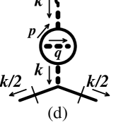
Figure 2: NLO diagrams (b) and (d) contributing to the exponent $\nu$, with explicit momentum assignment.

Secondly, diagram (d) (see Fig. 2 for momentum assignment) is evaluated in a similar way as

$${\rm(d)} \sim \left(\frac{6}{\lambda{\cal A}(\eta)}k^{1-2\eta}\right)^{2}\left(\frac{-\lambda}{6}\right)\int\frac{d^{3}p\,d^{3}q}{(2\pi)^{6}}\widetilde{G}({\boldsymbol{p}})\widetilde{G}({\boldsymbol{p}}+{\boldsymbol{k}})\left(\frac{-2}{N}\widetilde{\Pi}^{-1}({\boldsymbol{q}})\right)\widetilde{G}({\boldsymbol{p}}+{\boldsymbol{q}})\widetilde{G}({\boldsymbol{p}}+{\boldsymbol{q}}+{\boldsymbol{k}})$$

$$\sim \frac{6}{\lambda{\cal A}(\eta)}k^{1-2\eta}\left[\frac{k^{1-2\eta}}{{\cal A}^{2}(\eta)}\frac{2}{N}\int^{\Lambda}\frac{d^{3}p\,d^{3}q}{(2\pi)^{6}}\;p^{-2+\eta}|{\boldsymbol{p}}+{\boldsymbol{k}}|^{-2+\eta}|{\boldsymbol{p}}+{\boldsymbol{q}}|^{-2+\eta}|{\boldsymbol{p}}+{\boldsymbol{q}}+{\boldsymbol{k}}|^{-2+\eta}q^{1-2\eta}\right]$$

$$= \frac{6}{\lambda{\cal A}(\eta)}k^{1-2\eta}\left[\frac{2}{N{\cal A}(\eta)^{2}}\int^{\Lambda/k}\frac{d^{3}u\,d^{3}v}{(2\pi)^{6}}\;u^{-2+\eta}|{\boldsymbol{u}}+\hat{\boldsymbol{k}}|^{-2+\eta}|{\boldsymbol{u}}+{\boldsymbol{v}}|^{-2+\eta}|{\boldsymbol{u}}+{\boldsymbol{v}}+\hat{\boldsymbol{k}}|^{-2+\eta}v^{1-2\eta}\right]\,,$$

where we have rescaled the variables ${\boldsymbol{u}}={\boldsymbol{p}}/|{\boldsymbol{k}}|$, ${\boldsymbol{v}}={\boldsymbol{q}}/|{\boldsymbol{k}}|$ and $\hat{\boldsymbol{k}}={\boldsymbol{k}}/|{\boldsymbol{k}}|$. The $\ln k$ dependence comes from two regions of the above integral: (I) $|{\boldsymbol{v}}|\sim\Lambda/k$, $|{\boldsymbol{u}}|\ll|{\boldsymbol{v}}|$ and (II) $|{\boldsymbol{u}}|\sim|{\boldsymbol{v}}|\sim\Lambda/k$, $|{\boldsymbol{u}}+{\boldsymbol{v}}|\ll|{\boldsymbol{u}}|,\ |{\boldsymbol{v}}|$. One notices that the change of the variables, ${\boldsymbol{u}}^{\prime}={\boldsymbol{u}}+{\boldsymbol{v}}$ and ${\boldsymbol{v}}^{\prime}=-{\boldsymbol{v}}$, maps region II to region I and vice versa with keeping the integral the same, which means that these two regions give the same $\ln k$ contributions. Therefore, the $\ln k$ contribution in the above integral coincides with twice that from region I:

$${\rm(d)} \sim \frac{6}{\lambda{\cal A}(\eta)}k^{1-2\eta}\left[\frac{2}{N{\cal A}(\eta)^{2}}2\times\int_{\rm I}\frac{d^{3}u\,d^{3}v}{(2\pi)^{6}}\;u^{-2+\eta}|{\boldsymbol{u}}+\hat{\boldsymbol{k}}|^{-2+\eta}|{\boldsymbol{u}}+{\boldsymbol{v}}|^{-2+\eta}|{\boldsymbol{u}}+{\boldsymbol{v}}+\hat{\boldsymbol{k}}|^{-2+\eta}v^{1-2\eta}\right]$$ (53)

$$\sim \frac{6}{\lambda{\cal A}(\eta)}k^{1-2\eta}\left[\frac{4}{N{{\cal A}(\eta)}^{2}}\int^{\Lambda/k}\frac{d^{3}u\,d^{3}v}{(2\pi)^{6}}\,u^{-2+\eta}|{\boldsymbol{u}}+\hat{\boldsymbol{k}}|^{-2+\eta}v^{-3}\right]$$

$$= \frac{6}{\lambda{\cal A}(\eta)}k^{1-2\eta}\left[\frac{4}{N{{\cal A}(\eta)}^{2}}{{\cal A}(\eta)}\int^{\Lambda/k}\frac{d^{3}v}{(2\pi)^{3}}\,v^{-3}\right]$$

$$\sim \frac{6}{\lambda{\cal A}(\eta)}k^{1-2\eta}\left[\frac{-2}{\pi^{2}N{{\cal A}(\eta)}}\ln k\right].$$

Finally, we checked that both the coefficients in the diagrams (c) and (e) in Eq. (50) are consistent with zero in a numerical integration. Therefore, we do not include these two diagrams as alluded before. Details of the calculation are shown in Appendix. Notice that these two diagrams do not contribute to $\nu$ in the 1PI $1/N$ expansion Ma .

IV.2.3 Result

We collect the NLO corrections (52) and (53) to the LO result (47). As we noticed before, these NLO contributions (52) and (53) have the same prefactor $\widetilde{\Gamma}^{(2,1)}_{\rm LO}$. Therefore, we are able to exponentiate the $\ln k$ term to obtain $\widetilde{\Gamma}^{(2,1)}$ at the NLO:

$$\widetilde{\Gamma}^{(2,1)}_{\rm NLO}\left(\frac{{\boldsymbol{k}}}{2},\frac{{\boldsymbol{k}}}{2};{\boldsymbol{k}}\right) \sim \widetilde{\Gamma}^{(2,1)}_{\rm LO}\left(\frac{{\boldsymbol{k}}}{2},\frac{{\boldsymbol{k}}}{2};{\boldsymbol{k}}\right)\left[1-\frac{1}{\pi^{2}N{\cal A}(\eta)}\ln k\right]$$ (54)

$$\sim \frac{6}{\lambda{\cal A}(\eta)}\ k^{1-2\eta-\frac{1}{\pi^{2}N{\cal A}(\eta)}}\,.$$

Then, comparing this with Eq. (15), one finally obtains the exponent $\nu$ of the 2PI NLO calculation:

$$\nu^{\rm(2PI)}_{\rm NLO}=\frac{1}{1+\eta+\frac{1}{\pi^{2}N{\cal A}(\eta)}}\,,$$ (55)

where $\eta$ should be the 2PI critical exponent (43) for consistency. This is our main result. In the limit $N\to\infty$, this result of course recovers the LO result (48) together with $\lim_{N\to\infty}\eta(N)=0$. We plot $\nu$ as a function of $N$ in Fig. 3, where $\nu$ from the standard 1PI action at the NLO Ma

$$\nu^{\rm(1PI)}_{\rm NLO}=1-\frac{3\pi^{2}}{32N}$$ (56)

is also shown for comparison. At large $N$ the difference between the 1PI and 2PI results diminishes and both converge to the LO result $\nu_{\rm LO}=1$. At small $N$ the 2PI result stays positive, while the 1PI result can become negative. We see that the result of the 2PI NLO calculation gives an improved estimate for the exponent $\nu$ at $N=1,3$ than the 1PI NLO result.

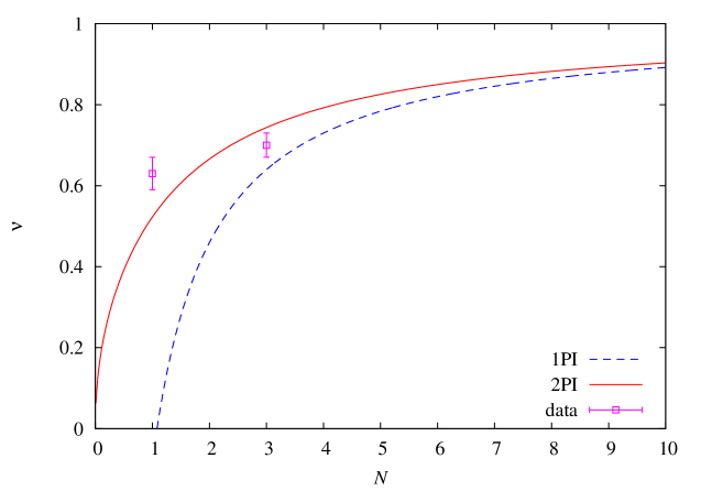
Figure 3: Exponent $\nu$ from 2PI NLO calculation as a function of $N$ (solid line). The result from 1PI NLO calculation (dashed line) and experimental data Chaikin are shown for comparison.

V summary and discussion

In the present paper we have developed a method to compute the critical exponent $\nu$ using the 2PI effective action. Although $\nu$ is associated with the diverging behavior of the correlation length $\xi$ near the critical point, one can compute it on the critical point by analyzing the three-point vertex function $\Gamma^{(2,1)}$. Roughly speaking, this is possible because $\Gamma^{(2,1)}$ is a derivative of the correlation function with respect to the temperature, and thus includes certain information on the deviation from the critical point. In the 2PI formalism we can write down a self-consistent equation for $\Gamma^{(2,1)}$, which is easily derived from the KB equation for the two-point function. The explicit form of the equation was obtained to the NLO in the $1/N$ expansion. We solved this equation by iteration to the NLO in the $1/N$ expansion, and identified from the resultant $\Gamma^{(2,1)}$ the exponent $\nu$, Eq. (55), as shown in Fig. 3.

The difference between the 2PI NLO result (55) and the 1PI NLO result (56) comes from two points as follows: Firstly, in the 2PI formalism, we deal with the full propagator in contrast to the free propagator in the 1PI formalism. Secondly, the sets of the NLO diagrams for $\Gamma^{(2,1)}$ are different between the 1PI and 2PI formalisms, while there is only one LO diagram which is common in both. Namely, the 1PI NLO calculation involves the following five diagrams Ma which should be compared with four 2PI diagrams shown in Eq. (50):

(57)

There is no self-energy insertion in the 2PI diagrams because it is already resummed in the full propagator. In fact, the first 1PI diagram contains one self-energy insertion, and is already included in the 2PI LO diagram Eq. (50) (a). This resummation of the self-energy diagrams in the 2PI formalism enables us to take account of important higher-order contributions into the form of the full propagator, which is the origin of the improvement of the 2PI result over the 1PI result in the calculation of the critical exponent.

Notice that the 1PI NLO result (56) has an apparent flaw at small $N$. The exponent $\nu$ must be positive $\nu>0$ as it describes the diverging behavior of the correlation length $\xi$ near the critical point (cf. Eq. (2)). However, the 1PI NLO result becomes negative at small $N$, although such a small value of $N$ is outside the validity region of the $1/N$ expansion in a strict sense. In contrast, the exponent $\nu$ in the 2PI NLO result remains positive for all $N$, and it is closer to the experimental data at $N=1,3$ Chaikin .

Expanding $\eta$ of Eq. (55) in $N$, we see that the 2PI result reproduces Ma’s 1PI result (56) Ma , and includes a part of higher order terms. It shows that the 2PI effective action resums not only leading-log-terms which are resummed in the 1PI calculation but also a certain class of the higer-log-terms.

In the present paper, we did not require the self-consistency for $\Gamma^{(2,1)}$, but rather solved the equation by iteration to the NLO. Using conformal invariance in the coordinate space Vasil'ev ; Vasil'ev et ; Polyakov in (28) at the critical point, one may analyze the self-consitent solution for $\Gamma^{(2,1)}$ to get a better estimate for $\nu$. However, one should keep in mind that the higher-order calculation of the exponent $\nu$ in the standard 1PI formalism up to ${\cal O}(1/N^{2})$ Justin ; AbeHikami tends to deviate from the experimental values. Inclusion of higher-order terms by requiring the self-consistency for $\Gamma^{(2,1)}$ is an open issue.

Appendix

Figure 4: NLO diagrams (c) and (e).

Here we show details of the calculation of diagrams (c) and (e) in Eq. (50). We closely follow Ref. Ma for identification and evaluation of the $\ln k$ contributions. With the momentum assingment shown in Fig. 4, each diagram is calculated as follows:

$${\rm(c)} \sim \frac{6}{\lambda{\cal A}(\eta)}k^{1-2\eta}\left[\frac{4}{N}\int\frac{d^{3}q}{(2\pi)^{3}}\widetilde{\Pi}^{-1}({\boldsymbol{q}})\widetilde{\Pi}^{-1}({\boldsymbol{q}}+{\boldsymbol{k}})\widetilde{G}({\boldsymbol{q}}+{\boldsymbol{k}}/2)T({\boldsymbol{k}},{\boldsymbol{q}})\right],$$ (58)

$${\rm(e)} \sim \frac{6}{\lambda{\cal A}(\eta)}k^{1-2\eta}\left[\frac{4}{N}\int\frac{d^{3}q}{(2\pi)^{3}}\widetilde{\Pi}^{-1}({\boldsymbol{q}})\widetilde{\Pi}^{-1}({\boldsymbol{q}}+{\boldsymbol{k}})T^{2}({\boldsymbol{k}},{\boldsymbol{q}})\left(\frac{-\lambda}{6}\cdot\frac{6}{\lambda}\Pi^{-1}({\boldsymbol{k}})\right)\right]$$ (59)

$$= \frac{6}{\lambda{\cal A}(\eta)}k^{1-2\eta}\left[\frac{-4}{N}\frac{k^{1-2\eta}}{{\cal A}(\eta)}\int\frac{d^{3}q}{(2\pi)^{3}}\widetilde{\Pi}^{-1}({\boldsymbol{q}})\widetilde{\Pi}^{-1}({\boldsymbol{q}}+{\boldsymbol{k}})T^{2}({\boldsymbol{k}},{\boldsymbol{q}})\right],$$

where $T({\boldsymbol{k}},{\boldsymbol{q}})$ represents the triangle part and is defined by

$$T({\boldsymbol{k}},{\boldsymbol{q}}) \equiv$$ (60)

$$= \int\frac{d^{3}p}{(2\pi)^{3}}\,\widetilde{G}({\boldsymbol{p}})\,\widetilde{G}({\boldsymbol{p}}+{\boldsymbol{k}})\,\widetilde{G}({\boldsymbol{p}}-{\boldsymbol{q}})$$

$$\sim \int\frac{d^{3}u}{(2\pi)^{3}}\,k^{-3+3\eta}\,{u}^{-2+\eta}\,|{\boldsymbol{u}}+\hat{{\boldsymbol{k}}}|^{-2+\eta}\,|{\boldsymbol{u}}-{\boldsymbol{v}}|^{-2+\eta}$$

$$\equiv k^{-3+3\eta}\,T_{0}(\hat{{\boldsymbol{k}}},{\boldsymbol{v}}).$$

Here we have again introduced dimensionless variables ${\boldsymbol{u}}={\boldsymbol{p}}/|{\boldsymbol{k}}|$, ${\boldsymbol{v}}={\boldsymbol{q}}/|{\boldsymbol{k}}|$, and $\hat{\boldsymbol{k}}={\boldsymbol{k}}/|{\boldsymbol{k}}|$. Then two diagrams become

$${\rm(c)} \sim \frac{6}{\lambda{\cal A}(\eta)}k^{1-2\eta}\left[\frac{4}{N}\int\frac{d^{3}v}{(2\pi)^{3}}v^{1-2\eta}|{\boldsymbol{v}}+\hat{{\boldsymbol{k}}}|^{1-2\eta}|{\boldsymbol{v}}+\hat{{\boldsymbol{k}}}/2|^{-2+\eta}\,T_{0}(\hat{{\boldsymbol{k}}},{\boldsymbol{v}})\right],$$ (61)

$${\rm(e)} \sim \frac{6}{\lambda{\cal A}(\eta)}k^{1-2\eta}\left[\frac{-4}{N{\cal A}(\eta)}\int\frac{d^{3}v}{(2\pi)^{3}}v^{1-2\eta}|{\boldsymbol{v}}+\hat{{\boldsymbol{k}}}|^{1-2\eta}T_{0}^{2}(\hat{{\boldsymbol{k}}},{\boldsymbol{v}})\right]\,.$$ (62)

As we disscuss in the text, we are interested in the $\ln k$ contribution when $k$ is small. We first note that the $\ln k$ contribution appears not from the integration over ${\boldsymbol{u}}$ in $T_{0}$, but from the integration over ${\boldsymbol{v}}$ in $T_{0}$. Instead, it will appear from the integration over ${\boldsymbol{v}}$. However, it is not straightforward to see the power of ${\boldsymbol{v}}$ from the above two expressions. If $T_{0}(\hat{{\boldsymbol{k}}},{\boldsymbol{v}})$ generates $v^{-3+3\eta}$, then $\ln k$ terms appear in Eq. (61);

$$T_{0}(\hat{\boldsymbol{k}},{\boldsymbol{v}})\sim v^{-3+3\eta} \rightarrow {\rm(c)}\sim\int^{\Lambda/k}dvv^{-1}\sim\ln k.$$ (63)

Similarly, in Eq. (62), if $T_{0}^{2}(\hat{{\boldsymbol{k}}},{\boldsymbol{v}})$ yields $v^{-5+4\eta}$, then $\ln k$ terms appear;

$$T_{0}^{2}(\hat{{\boldsymbol{k}}},{\boldsymbol{v}})\sim v^{-5+4\eta} \rightarrow {\rm(e)}\sim\int^{\Lambda/k}dvv^{-1}\sim\ln k.$$ (64)

Below we examine whether these powers indeed appear in $T$. The definition of $T_{0}$ in Eq. (60) can be explicitly written as ($\theta$ and $\phi$ are the angles between two vectors $({\boldsymbol{u}},\hat{\boldsymbol{k}})$ and $({\boldsymbol{u}},{\boldsymbol{v}})$, respectively)

$$T_{0}(\hat{{\boldsymbol{k}}},{\boldsymbol{v}}) = \frac{1}{8\pi^{3}}\int u^{2}du\int d\Omega\,u^{-2+\eta}(u^{2}+2u\cos\theta+1)^{-1+\eta/2}(u^{2}+2uv\cos\phi+v^{2})^{-1+\eta/2}.$$ (65)

To see the power of $v$ in this quantity, it is convenient to perform the Mellin transformation defined by

$$g(s) = \int_{0}^{\infty}dxf(x)x^{s-1},$$ (66)

$$f(x) = \frac{1}{2\pi i}\int_{c-i\infty}^{c+i\infty}dsx^{-s}g(s)\,.$$ (67)

The $v$-dependent part of Eq. (65) can be Mellin-transformed as follows:

$$\int_{0}^{\infty}dv(u^{2}+2uv\cos\phi+v^{2})^{-1+\eta/2}v^{s-1} = 2^{1/2-\eta/2}(\sin\phi)^{\eta/2-1/2}\frac{\Gamma(s)\Gamma(2-\eta-s)}{\Gamma(2-\eta)}\left(\frac{1+\cos\phi}{1-\cos\phi}\right)^{\eta/4-1/4}$$ (68)

$$\times{}_{2}F_{1}\left(-s-\frac{\eta}{2}+\frac{3}{2},s+\frac{\eta}{2}-\frac{1}{2},-\frac{\eta}{2}+\frac{3}{2},\frac{1-\cos\phi}{2}\right)$$

$$\times u^{s+\eta-2}$$

$$\equiv F(s,\eta,\phi)u^{s+\eta-2},\ \ \ \ \ (0<{\rm Re}[s]<2-\eta)$$

where $B$ is the beta function, $P_{\mu}^{\lambda}$ is the associated Legendre function and $F$ is the hypergeometric function. Here we have used the formula formula ($0<{\rm Re}[s]<2\mu,\ -\pi<\theta<\pi$):

$$\int_{0}^{\infty}(x^{2}+2ax\cos\theta+a^{2})^{-\mu}x^{s-1}dx = 2^{\mu-1/2}(\sin\theta)^{1/2-\mu}\Gamma\left(\mu+\frac{1}{2}\right)B(s,2\mu-s)P_{s-\mu-1/2}^{1/2-\mu}(\cos\theta)a^{s-2\mu}$$ (69)

$$= 2^{\mu-1/2}(\sin\theta)^{1/2-\mu}\frac{\Gamma(s)\Gamma(2\mu-s)}{\Gamma(2\mu)}\left(\frac{1+\cos\theta}{1-\cos\theta}\right)^{1/4-\mu/2}$$

$$\times{}_{2}F_{1}\left(-s+\mu+\frac{1}{2},s-\mu+\frac{1}{2},\mu+\frac{1}{2},\frac{1-\cos\theta}{2}\right)a^{s-2\mu}\,.$$

Therefore, Mellin transform of Eq. (65) is given as

$$T_{0}(\hat{{\boldsymbol{k}}},s) = \int_{0}^{\infty}dvT_{0}(\hat{{\boldsymbol{k}}},{\boldsymbol{v}})v^{s-1}$$ (70)

$$= \frac{1}{8\pi^{3}}\int_{0}^{\infty}u^{2}du\int d\Omega\,u^{-2+\eta}(u^{2}+2u\cos\theta+1)^{-1+\eta/2}F(s,\eta,\phi)u^{s+\eta-2}$$

$$= \frac{1}{8\pi^{3}}\int d\Omega F(s,\eta,\phi)\int_{0}^{\infty}duu^{s+2\eta-2}(u^{2}+2u\cos\theta+1)^{-1+\eta/2}.$$

If we use the formula (69) again, then Eq. (68) becomes

$$\int_{0}^{\infty}duu^{s+2\eta-2}(u^{2}+2u\cos\theta+1)^{-1+\eta/2} = 2^{1/2-\eta/2}(\sin\theta)^{\eta/2-1/2}\frac{\Gamma(s+2\eta-1)\Gamma(3-3\eta-s)}{\Gamma(2-\eta)}$$ (71)

$$\times\left(\frac{1+\cos\theta}{1-\cos\theta}\right)^{\eta/4-1/4}$$

$$\times{}_{2}F_{1}\left(-s-\frac{5\eta}{2}+\frac{5}{2},s+\frac{5\eta}{2}-\frac{3}{2},-\frac{\eta}{2}+\frac{3}{2},\frac{1-\cos\theta}{2}\right)$$

$$\equiv F^{\prime}(s,\eta,\theta),\ \ \ \ \ (1-2\eta<{\rm Re}[s]<3-3\eta).$$

Therefore, Eq. (65) can be written as

$$T_{0}(\hat{{\boldsymbol{k}}},s) = \frac{1}{8\pi^{3}}\int d\Omega F(s,\eta,\phi)F^{\prime}(s,\eta,\theta),\ \ \ \ \ (1-2\eta<{\rm Re}[s]<2-\eta).$$ (72)

Performing the inverse Mellin transformation, we obtain

$$T_{0}({\hat{\boldsymbol{k}}},{\boldsymbol{v}}) = \frac{1}{2\pi i}\int_{c-i\infty}^{c+i\infty}dsT_{0}(\hat{{\boldsymbol{k}}},s)v^{-s}$$ (73)

$$= \frac{1}{2\pi i}\int_{c-i\infty}^{c+i\infty}ds\frac{1}{8\pi^{3}}\int d\Omega F(s,\eta,\phi)F^{\prime}(s,\eta,\theta)v^{-s},$$

where $1-2\eta<c<2-\eta$. For the integration over $s$, we close the integration path in the right semicircle. Then, the poles of $F(s,\eta,\phi)$ and $F^{\prime}(s,\eta,\theta)$ are, respectively, at

$$s= 2-\eta,\ 3-\eta,\ \cdots,$$ (74)

$$s= 3-3\eta,\ 4-3\eta,\ \cdots.$$ (75)

Poles we are now interested in are $s=2-\eta$ for diagram (c), and $s=3-3\eta$ for diagram (e) which yield the $\ln k$ contributions (see Eqs. (63), (64)). Below we evaluate $T_{0}(\hat{\boldsymbol{k}},{\boldsymbol{v}})$ only at these poles.

First consider the pole $s=2-\eta$. Since the residue of the gamma function at $z=-n$ is

$$\lim_{z\to-n}(z+n)\Gamma(z)=\frac{(-1)^{n}}{n!},$$ (76)

Residues of $F$ and $F^{\prime}$ at $s=2-\eta$ can be evaluated as

$$\lim_{s\to 2-\eta}(s-2+\eta)F(s,\eta,\phi) = 2^{1/2-\eta/2}\,\frac{1}{2}\left(\cos\frac{\phi}{2}\right)^{-1-\eta}(1+\cos\phi)^{1/2+\eta/2}=1,$$ (77)

$$\lim_{s\to 2-\eta}(s-2+\eta)F^{\prime}(s,\eta,\theta) = 2^{1/2-\eta/2}(1+\cos\theta)^{\eta/2-1/2}\frac{\Gamma(1+\eta)\Gamma(1-2\eta)}{\Gamma(2-\eta)}$$ (78)

$$\times{}_{2}F_{1}\left(\frac{1-3\eta}{2},\frac{1+3\eta}{2},\frac{3-\eta}{2},\frac{1-\cos\theta}{2}\right).$$

Substituting these into Eq. (73), we get

$$\frac{1}{8\pi^{3}}\int d\Omega F(s,\eta,\phi)F^{\prime}(s,\eta,\theta)v^{-2+\eta} = \frac{1}{4\pi^{2}}\int_{-1}^{1}d\cos\theta 2^{1/2-\eta/2}(1+\cos\theta)^{\eta/2-1/2}\frac{\Gamma(1+\eta)\Gamma(1-2\eta)}{\Gamma(2-\eta)}$$ (79)

$$\times{}_{2}F_{1}\left(\frac{1-3\eta}{2},\frac{1+3\eta}{2},\frac{3-\eta}{2},\frac{1-\cos\theta}{2}\right)v^{-2+\eta}$$

$$\equiv L_{1}v^{-2+\eta}.$$

Next, consider the other pole at $s=3-3\eta$. Then,

$$\lim_{s\to 2-\eta}(s-3+3\eta)F(s,\eta,\phi) = 2^{1/2-\eta/2}\,(1+\cos\phi)^{\eta/2-1/2}\frac{\Gamma(3-3\eta)\Gamma(-1+2\eta)}{\Gamma(2-\eta)}$$ (80)

$$\times{}_{2}F_{1}\left(\frac{5-5\eta}{2},\frac{-3+5\eta}{2},\frac{3-\eta}{2},\frac{1-\cos\phi}{2}\right),$$

$$\lim_{s\to 2-\eta}(s-3+3\eta)F^{\prime}(s,\eta,\theta) = 1\,.$$ (81)

Therefore, Eq. (73) becomes

$$\frac{1}{8\pi^{3}}\int d\Omega F(s,\eta,\phi)F^{\prime}(s,\eta,\theta)v^{-3+3\eta} = \frac{1}{4\pi^{2}}\int_{-1}^{1}d\cos\phi 2^{1/2-\eta/2}(1+\cos\phi)^{\eta/2-1/2}\frac{\Gamma(3-3\eta)\Gamma(-1+2\eta)}{\Gamma(2-\eta)}$$ (82)

$$\times{}_{2}F_{1}\left(\frac{5-5\eta}{2},\frac{-3+5\eta}{2},\frac{3-\eta}{2},\frac{1-\cos\phi}{2}\right)v^{-3+3\eta}$$

$$\equiv L_{2}v^{-3+3\eta}.$$

As a result, $T_{0}$ becomes

$$T_{0}({\hat{\boldsymbol{k}}},{\boldsymbol{v}})=L_{1}v^{-2+\eta}+L_{2}v^{-3+3\eta}+(\mbox{higer order}),$$ (83)

and the contribution of diagram (c) is

$${\rm(c)} \sim \frac{6}{\lambda{\cal A}(\eta)}k^{1-2\eta}\left[\frac{4}{N}\int\frac{d^{3}v}{8\pi^{3}}v^{1-2\eta}|{\boldsymbol{v}}+{\hat{\boldsymbol{k}}}|^{1-2\eta}\,|{\boldsymbol{v}}+{\hat{\boldsymbol{k}}}/2|^{-2+\eta}\,T_{0}({\hat{\boldsymbol{k}}},{\boldsymbol{v}})\right]$$ (84)

$$\sim \frac{6}{\lambda{\cal A}(\eta)}k^{1-2\eta}\left[\frac{4}{N}\int^{\Lambda/k}\frac{d^{3}v}{8\pi^{3}}v^{1-2\eta}|{\boldsymbol{v}}+{\hat{\boldsymbol{k}}}|^{1-2\eta}|{\boldsymbol{v}}+{\hat{\boldsymbol{k}}}/2|^{-2+\eta}L_{2}v^{-3+3\eta}\right]$$

$$\sim \frac{6}{\lambda{\cal A}(\eta)}k^{1-2\eta}\left[\frac{4L_{2}}{N}\frac{1}{2\pi^{2}}\ln\frac{\Lambda}{k}\right]\,.$$

Similarly, diagram (e) is

$${\rm(e)} \sim \frac{6}{\lambda{\cal A}(\eta)}k^{1-2\eta}\left[\frac{-4}{N{\cal A}(\eta)}\int\frac{d^{3}v}{8\pi^{3}}v^{1-2\eta}|{\boldsymbol{v}}+{\hat{\boldsymbol{k}}}|^{1-2\eta}\,T^{2}_{0}({\hat{\boldsymbol{k}}},{\boldsymbol{v}})\right]$$ (85)

$$\sim \frac{6}{\lambda{\cal A}(\eta)}k^{1-2\eta}\left[\frac{-4}{N{\cal A}(\eta)}\int\frac{d^{3}v}{8\pi^{3}}v^{1-2\eta}|{\boldsymbol{v}}+{\hat{\boldsymbol{k}}}|^{1-2\eta}L_{1}L_{2}v^{-5+4\eta}\right]$$

$$= \frac{6}{\lambda{\cal A}(\eta)}k^{1-2\eta}\left[\frac{-4L_{1}L_{2}}{N{\cal A}(\eta)}\frac{1}{2\pi^{2}}\ln\frac{\Lambda}{k}\right].$$

Notice that both diagrams (c) and (e) have the similar structure as those of diagrams (b) and (d). What remains is the estimation of the coefficients $L_{1}$ and $L_{2}$. We evaluated $L_{1}$ and $L_{2}$ numerically, and found that $L_{1}\sim{\cal O}(1)$ while $L_{2}$ is consistent with zero. Therefore, we conclude that diagrams (c) and (e) could have the $\ln k$ contributions, but are numerically very small, and can be ignored in our calculation.

References

- (1) E. A. Calzetta and B. B. Hu, Nonequilibrium Quantum Field Theory (Cambridge, 2008).
- (2) D. Boyanovsky, H. J. de Vega and D. J. Schwarz, Ann. Rev. Nucl. Part. Sci. 56 (2006) 441 [arXiv:hep-ph/0602002].
- (3) P. C. Hohenberg and B. I. Halperin, Rev. Mod. Phys. 49, 435 (1977).
- (4) G. F. Mazenko, Nonequilibrium Statistical Mechanics (Wiley-VCH, 2006).
- (5) L. M. Luttinger and J. C. Ward, Phys. Rev. 118, 1417 (1960).
- (6) J. M. Cornwall, R. Jackiw and E. Tomboulis, Phys. Rev. D 10, 2428 (1974).
- (7) M. Alford, J. Berges and J. M. Cheyne, Phys. Rev. D 70, 125002 (2004).
- (8) J. Berges, S. Schlichting and D. Sexty, Nuc. Phys. B 832 228 (2010).
- (9) J. Berges, AIP Conf. Proc. 739, 3 (2005) and references therein.
- (10) L. P. Kadanoff and G. Baym, Phys. Rev. 124, 287 (1961).
- (11) G. Baym, Phys. Rev. 127, 1391 (1962).
- (12) L. P. Kadanoff and G. Baym, Quantum Statistical Mechanics, (Westview Press, 1989).
- (13) D. J. Amit and V. M. Mayor, Field Theory, the Renormalization Group, and Critical Phenomena: Graphs to Computers (World Scientific, 2005).
-
(14)
K. G. Wilson, Phys. Rev. B 4, 3174 (1971); ibid., 3184;
K. G. Wilson and M. E. Fisher, Phys. Rev. Lett. 28, 240 (1972). - (15) S. Ma, Phys. Rev. A 7, 2172 (1973).
- (16) S. Ma, Rev. Mod. Phys. 45, 589 (1973).
- (17) S. Ma, Modern Theory of Critical Phenomena (Perseus, 2000).
- (18) R. Abe and S. Hikami, Prog. Theor. Phys. 49 No.1 (1973) 113.
- (19) A. N. Vasil’ev, The Field Theoretic Renormalization Group in Critical Behavior Theory and Stochastic Dynamics, (CRC press, 2004).
- (20) J. Z. Justin, Quantum Field Theory and Critical Phenomena (4th ed. Oxford Univ. Press, 2002).
- (21) H. van Hees and J. Knoll, Phys. Rev. D66, 025028 (2002).
- (22) P. M. Chaikin and T. C. Lubensky, Principles of Condensed Matter Physics, (Cambridge, 2000).
- (23) A. M. Polyakov, JETP Lett. 12, 381 (1970).
- (24) A. N. Vasil’ev, M. M. Perekalin and Y. M. Pis’mak, Theor. Math. Phys. 55, 529 (1983).
- (25) A. Erdelyi (ed.) Tables of integral transforms (McGraw-Hill, NY, 1954).