Automized Squark–Neutralino Production to Next-to-Leading Order

Abstract

The production of one hard jet in association with missing transverse energy is a major LHC search channel motivated by many scenarios for physics beyond the Standard Model. In scenarios with a weakly interacting dark matter candidate, like supersymmetry, it arises from the associated production of a quark partner with the dark matter agent. We present the next-to-leading order cross section calculation as the first application of the fully automized MadGolem package. We find moderate corrections to the production rate with a strongly reduced theory uncertainty.

I Introduction

Since the LHC started running at a center-of-mass energy of 7 TeV searches for new physics are a major effort, realized in a rapidly increasing number of publications review . Inclusive searches for supersymmetry at the LHC have started to constrain the allowed parameter space of the minimal supersymmetric Standard Model susy_lhc , most notably in the part of the squark–gluino mass plane which can be described in terms of gravity mediation. Such searches are based on jet production from squark and gluino decays and two stable lightest supersymmetric particles (LSP). The latter could be a dark matter agent with a weak-scale mass.

The main production mode for jets and dark matter particles at the LHC would most likely be squark or gluino pair production, mediated by the strong interaction autofocus . The limitation of this channel is that it will be hard to extract any model parameters beyond the masses of the new particles sfitter_fittino . The production is governed by the strong interaction and the (sum of) branching ratio(s) leading to jets plus missing transverse energy can be expected to be close to unity. Therefore, it is worth studying additional production processes which directly involve the weakly interacting sector of the new physics model. In supersymmetry, those are the associated production of a gluino gluino_asso or a squark with a neutralino or chargino squark_asso

$$pp\;\to\;\tilde{q}\tilde{\chi}_{,}^{0}\quad\tilde{q}\tilde{\chi}^{\pm}\;.$$ (1)

The leading order Feynman diagrams for this process we show in Fig. 1. This channel naturally leads to one single hard decay jet and missing energy. This signature is not unique to supersymmetry or other models with quark partners and a weakly interacting dark matter agent; it also constitutes the theoretically most reliable signature for large extra dimensions extrad . In that sense, observing single jet production with missing energy would be one of the most exciting anomalies to interpret at the LHC.

Figure 1: Feynman diagrams for the associated production of a squark and a gaugino to leading order.

Aside from the quark-gluon and squark-gluon QCD vertices, the leading-order process is driven by the $q$-$\tilde{q}$-$\tilde{\chi}$ interaction. Because the dominant light-flavor quarks only have a tiny Yukawa coupling, this interaction relies on the two weak gauge charges of the quark-squark pair involved. This way, it carries information on the composition of the dark matter candidate $\tilde{\chi}_{1}^{0}$ and an accurate measurement would also allow improved predictions for the direct detection and relic density of dark matter. Finally, this process probes the supersymmetric relations between the gauge couplings and the gaugino-quark-squark couplings. Prospects for carrying out such a measurement out of the mono-jet rates at the LHC have been studied in Ref. Allanach:2010pp .

Next-to-leading order QCD contributions to this production process arise at order $\alpha\alpha_{s}^{2}$ and originate from both QCD (gluon mediated) and SUSY-QCD (gluino mediated) contributions. They involve virtual one-loop corrections as well as real emission off the initial state partons or the final state squark. While we expect the size of the virtual corrections combined with real emission to stay moderate, there are potential sources of huge corrections; for example, the production of a squark pair where one of the two squarks decays to a quark and a neutralino contributes at the same order $\alpha\alpha_{s}^{2}$, but can effectively be an overwhelming two particle production process. To avoid double counting and instead allow for a clear separation and prediction of the two channels, the treatment of on-shell singularities in associated squark and neutralino production is crucial. Note that this separation without double counting serves a theoretical purpose. For an actual observable, we always need to combine QCD pair production with associated production because initial state jet radiation at the LHC can be as hard as decay jets qcd_radiation and cannot be distinguished event by event.

Finally, we use this production process to show how heavy particle pairs at next-to-leading order can be described by the fully automized tool MadGolem. It generates all tree-level diagrams and the corresponding helicity amplitudes in the Madgraph framework madgraph , based on Helas helas . The virtual corrections are generated with Qgraf qgraf and numerically computed by Golem golem . Supersymmetric counter terms are part of the model implementation. On-shell subtraction terms in the Prospino scheme prospino_squark ; thesis ; prospino_onshell can also be generated automatically. Further details we provide in the appendix. To our knowledge, this process is the first fully automized beyond-the-Standard-Model next-to-leading order (NLO) computation based on a (soon-to-be) public add-on to a major Monte Carlo generator, meant to be used independently by the LHC experimental community.

II S-up production in association with the LSP

In this first section we focus on total rates for $\tilde{u}_{R}\tilde{\chi}_{1}^{0}$ and $\tilde{u}_{L}\tilde{\chi}_{1}^{0}$ production and features characterizing the NLO effects. The results we present in terms of the consistent ratio $K=\sigma^{\text{NLO}}/\sigma^{\text{LO}}$, an approach which we will modify once we study distributions in Sec. III.

To avoid the current LHC bounds on squark and gluino production susy_lhc we use a modified SPS1a sps point (SPS1a₁₀₀₀) where the gluino mass is increased to $1~{}{\rm TeV}$. Because the gluino does not appear in the LO Feynman diagrams, its increased mass will merely reduce the impact of SUSY-QCD corrections which are nevertheless fully included — some effective theory issues with the proper decoupling of the gluino we discuss in detail later.

In our numerical analysis we use the CTEQ6L1 and CTEQ6M parton densities with five flavors cteq . For the strong coupling we consistently rely on the corresponding $\alpha_{s}(\mu_{R})$. Its value we compute using two-loop running from $\Lambda_{\text{QCD}}$ to the required renormalization scale, again with five active flavors. For the central renormalization and factorization scales we use the average final state mass $\mu_{R}^{0}=\mu_{F}^{0}=(m_{\tilde{q}}+m_{\tilde{\chi}})/2$, which has been shown to lead to stable perturbative results prospino_squark ; prospino_chargino .

$\sqrt{S}\,[{\rm TeV}]$		$\sigma^{\text{LO}}$ [fb]	$\sigma^{\text{NLO}}$ [fb]	$K$		$\sigma^{\text{LO}}$ [fb]	$\sigma^{\text{NLO}}$ [fb]	$K$	$m_{\tilde{q}_{R}}\,[{\rm GeV}]$	$m_{\tilde{q}_{L}}\,[{\rm GeV}]$
7	$\tilde{u}_{R}\,\tilde{\chi}_{1}^{0}$	29.62	42.17	1.42	$\tilde{u}_{L}\,\tilde{\chi}_{1}^{0}$	0.83	1.26	1.52	549	561
14		176.36	245.74	1.39		5.03	7.52	1.49
7	$\tilde{d}_{R}\,\tilde{\chi}_{1}^{0}$	3.61	5.31	1.47	$\tilde{d}_{L}\,\tilde{\chi}_{1}^{0}$	1.21	1.77	1.46	545	568
14		24.89	35.50	1.43		8.67	12.37	1.43
7	$\tilde{c}_{R}\,\tilde{\chi}_{1}^{0}$	1.12	1.81	1.61	$\tilde{c}_{L}\,\tilde{\chi}_{1}^{0}$	0.03	0.06	2.00	549	561
14		13.69	20.69	1.51		0.38	0.66	1.70
7	$\tilde{s}_{R}\,\tilde{\chi}_{1}^{0}$	0.57	0.78	1.38	$\tilde{s}_{L}\,\tilde{\chi}_{1}^{0}$	0.19	0.29	1.56	545	568
14		5.86	8.45	1.44		2.00	2.98	1.49
7	$\sum\tilde{q}_{R}\,\tilde{\chi}_{1}^{0}$	34.92	50.07	1.43	$\sum\tilde{q}_{L}\,\tilde{\chi}_{1}^{0}$	2.26	3.38	1.50
14		220.80	310.38	1.41		16.08	23.53	1.46

Table 1: Individual production rates $\sigma(pp\to\tilde{q}\tilde{\chi}_{1}^{0})$ and corresponding $K$ factors for the modified SPS1a₁₀₀₀  scenario. The first and second generation squark masses happen to be degenerate. The scales are set to their central values $\mu_{R}^{0}=\mu_{F}^{0}=(m_{\tilde{q}}+m_{\tilde{\chi}^{0}_{1}})/2$. In the last line we show the sum of all contributions.

Before we discuss the features of the NLO corrections in detail for the (dominant) $\tilde{u}\tilde{\chi}_{1}^{0}$ production channel, in Tab. 1 we quote the individual cross sections for all light-flavor $\tilde{q}\tilde{\chi}_{1}^{0}$ channels.

The results in Tab. 1 clearly reflect the flavor-locked nature of the process; ordered by the squark flavor in the final state, all contributions stemming from sea quarks are essentially irrelevant. Our single jet signature is driven by the $\tilde{u}$ and $\tilde{d}$ contributions, with the second generation contributing at the $5\%$ level and, as we will see, within the NLO scale uncertainty. Bottom-induced sbottom production we expect to be further suppressed even though moderately large collinear logarithms might enhance such a signature for very light sbottoms.

In addition, the modified SPS1a parameter point is a fairly generic scenario for the weak sector and accommodates a relatively light mostly bino LSP. As a consequence, the neutralino coupling strength to the right and left squarks is substantially different, i.e.  $g_{u\tilde{u}_{L}\tilde{\chi}_{1}^{0}}/g_{u\tilde{u}_{R}\tilde{\chi}_{1}^{0}}\simeq 0.176\sim 1/6$. This explains the difference between the LO cross sections for $\tilde{u}_{L}\tilde{\chi}_{1}^{0}$ and $\tilde{u}_{R}\tilde{\chi}_{1}^{0}$ production of roughly one order of magnitude. As a bottom line, we see that for a bino LSP more than 80% of the total squark-LSP production rates comes from the $\tilde{u}_{R}\tilde{\chi}_{1}^{0}$ contribution.

II.1 Real and virtual corrections

Figure 2: Cross sections $\sigma(pp\to\tilde{u}_{R/L}\tilde{\chi}_{1}^{0})$ (top panels) and $K$ factor (bottom panels) as a function of $m_{\tilde{u}_{R/L}}$ assuming $m_{\tilde{u}_{L}}-m_{\tilde{u}_{R}}=20\,{\rm GeV}$. For negative contributions to the total rate we show $|\sigma|$. The remaining MSSM parameters are fixed to our benchmark point. Real and the virtual corrections are separated using the original Catani-Seymour dipoles catani_seymour with $\alpha=1$, the integrated dipoles are included in the virtual corrections. The LHC energy is 7 TeV.

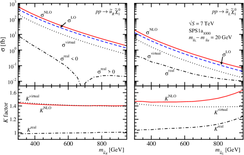
In Fig. 2 we show the total cross sections as a function of the squark mass. To assess the relative impact of the real emission versus virtual corrections, and to spell out the differences between the right and left squarks, we only show results for $\tilde{u}_{R}\tilde{\chi}_{1}^{0}$ and $\tilde{u}_{L}\tilde{\chi}_{1}^{0}$ production. The former drives the bulk of the overall $\tilde{q}\tilde{\chi}_{1}^{0}$ event rate. The two up squark masses we vary simultaneously with a fixed splitting $m_{\tilde{u}_{L}}-m_{\tilde{u}_{R}}=20\,{\rm GeV}$. As we can see, the virtual corrections are the dominant NLO effects, leading to a NLO correction of the order $K\sim 1.4$.

As real corrections we consider all contributions to the NLO cross section with a three-particle final state. Virtual corrections include gluon and gluino induced loops, but also integrated dipoles following the Catani-Seymour dipole prescription catani_seymour . While the dipole subtraction always covers the soft and collinearly divergent phase space regions, in terms of a variable parameter $\alpha$ they can be defined to extend more ($\alpha=1$) or less ($\alpha\ll 1$) into the non-divergent phase space regime alpha . Unlike for the distributions shown in Sec. III in this section we use $\alpha=1$, as in the original implementation.

Given this choice, in Fig. 2 we see that real corrections are generally small compared to their virtual counterparts. They exhibit an interesting feature, namely a positive (negative) contribution for the $\tilde{u}_{L}\tilde{\chi}_{1}^{0}$ ($\tilde{u}_{R}\tilde{\chi}_{1}^{0}$) channel. We can understand this feature through the different couplings to the neutralino: real corrections to the $\tilde{u}_{L}\tilde{\chi}_{1}^{0}$ channel mainly depend on $g_{u\tilde{u}_{L}\tilde{\chi}_{1}^{0}}$, but at next-to-leading order also $g_{u\tilde{u}_{R}\tilde{\chi}_{1}^{0}}$ contributes. For example, this happens for real corrections triggered by the $gg,uu$ and $u\bar{u}$ initial states, as shown in Fig. 3. This way, the NLO production rates no longer factorize with the LO quark-squark-neutralino coupling. Such higher order effects are sensitive to the coupling imbalance at our parameter point, recalling $g_{u\tilde{u}_{R}\tilde{\chi}_{1}^{0}}/g_{u\tilde{u}_{L}\tilde{\chi}_{1}^{0}}\simeq 6$ owing to the bino-like nature of the LSP dark matter candidate. This is why the real corrections to the $\tilde{u}_{R}\tilde{\chi}_{1}^{0}$ channel are much smaller, and of the opposite sign than for the $\tilde{u}_{L}\tilde{\chi}_{1}^{0}$ channel.

Figure 3: Example Feynman diagrams for real emission corrections to $\tilde{q}_{R}\tilde{\chi}^{0}$ production via intermediate on-shell states.

II.2 Renormalization

Before we describe the MadGolem combination of the virtual and real corrections we need to ensure that ultraviolet and infrared divergences are properly separated. A crucial ingredient to our higher order calculation therefore is the automatic treatment of the ultraviolet divergences, i.e.  renormalization. In the partonic LO cross section there appear three parameters which require renormalization in QCD or SUSY-QCD. First, the squark mass is renormalized in the on-shell scheme, which means that all contributions from gluon or gluino exchange are absorbed into the mass counter term. For QCD corrections this scheme can be fully extended to mixing squarks stop_dec ; thesis , but in this work we assume the squark mixing angle to lead to negligible effects. Second, we renormalize the strong coupling constant in the five-flavor $\overline{\text{MS}}$ scheme and explicitly decouple the heavier colored particles from its running. This zero-momentum subtraction scheme prospino_squark ; Berge:2007dz leaves the renormalization group running of $\alpha_{s}$ to be determined only by the lightest colored particles. It corresponds to the definition of the measured value of the strong coupling, for example in a combined fit with the parton densities. The renormalization constant then reads

$$\delta\,Z_{g_{s}}=-\frac{\alpha_{s}}{4\pi}\;\frac{\beta^{L}_{0}+\beta^{H}_{0}}{2}\,\Delta_{\epsilon}-\frac{\alpha_{s}}{4\pi}\,\left(\frac{1}{3}\,\log\frac{m^{2}_{t}}{\mu_{R}^{2}}+\log\frac{m^{2}_{\tilde{g}}}{\mu_{R}^{2}}+\frac{1}{12}\,\sum_{\text{12 squarks}}\,\log\frac{m^{2}_{\tilde{q}_{j}}}{\mu_{R}^{2}}\right)\;,$$ (2)

in terms of $\Delta_{\epsilon}=1/\epsilon-\gamma_{E}+\log(4\pi)$. The coefficient of the QCD beta function we can decompose into contributions from light and heavy particles, $\beta_{0}=\beta^{L}_{0}+\beta_{0}^{H}$, with

$$\beta_{0}^{L}=\left[\frac{11}{3}\,C_{A}-\frac{2}{3}\,n_{f}\right]\qquad\qquad\text{and}\qquad\beta_{0}^{H}=\left[-\frac{2}{3}-\frac{2}{3}\,C_{A}-\frac{1}{3}\,(n_{f}+1)\right]\;.$$ (3)

The number of active flavors is $n_{f}=5$. Correspondingly, the gluon field renormalization constant can be written as

$$\delta\,Z_{G}=-\frac{\alpha_{s}}{4\pi}\;\left(\beta^{L}_{0}+\beta^{H}_{0}\right)\,\Delta_{\epsilon}+\frac{\alpha_{s}}{2\pi}\,\left(\frac{1}{3}\,\log\frac{m^{2}_{t}}{\mu_{R}^{2}}+\log\frac{m^{2}_{\tilde{g}}}{\mu_{R}^{2}}+\frac{1}{12}\,\sum_{\text{12 squarks}}\,\log\frac{m^{2}_{\tilde{q}_{j}}}{\mu_{R}^{2}}\right).$$ (4)

Reflecting the underlying Slavnov-Taylor identities, the finite parts of both renormalization constants are related as $\delta\,Z_{G}=-2\,\delta\,Z_{g_{s}}$.

Finally, we need to compensate for dimensional regularization and the $\overline{\text{MS}}$ scheme breaking supersymmetry through the mismatch of two gaugino and $D-2=2-2\epsilon$ gauge vector degrees of freedom Martin:1993yx ; signer_stoeckinger . This is done by a finite SUSY-restoring counter term in the quark-squark-gaugino Yukawa coupling $g_{q\tilde{q}\tilde{\chi}}$ with respect to the associated gauge coupling. For the $q$-$\tilde{q}$-$\tilde{\chi}$ coupling, this prescription translates into a shift in $g_{2}=e/s_{w}$ prospino_chargino . The SUSY-restoring counter terms can be computed using dimensional reduction, i.e.  the $\overline{\text{DR}}$ scheme.

The fact that the $q$-$\tilde{q}$-$\tilde{\chi}$ couplings has a supersymmetric limit means that we cannot numerically decouple the gluino contribution from this process and obtain something like a scalar leptoquark limit. While this limit is perfectly renormalizable, a very heavy gluino breaks supersymmetry and the ultraviolet structure of the coupling. We have checked that to decouple the gluinos we have to absorb a logarithm $\log m_{\tilde{g}}$ into an explicit decoupling decouple , in analogy to Eq. 2.

II.3 On-shell subtraction

Figure 4: NLO contributions from intermediate on-shell particles contributing to $\tilde{u}_{R}\tilde{\chi}_{1}^{0}$ production in the $uu$ initial state. We show the behavior as a function of the width-to-mass ratio $\Gamma_{\tilde{u}}/m_{\tilde{u}}$ of the on-shell squark, which acts as a mathematical cutoff in the Prospino subtraction scheme prospino_onshell , see the text for details. The masses are different from our usual benchmark point, to illustrate all different channels. The LHC energy is 14 TeV. Virtual corrections are not included.

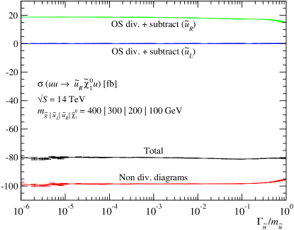
The Feynman diagrams in Fig. 3 naively lead to very large corrections to the Born process. The reason is that for on-shell intermediate states we would compare a $2\to 2$ leading order process proportional to $\alpha\alpha_{s}$ with a next-to-leading $2\to 2$ contribution proportional to $\alpha_{s}^{2}$, multiplied by a branching ratio which can be close to unity. However, the same diagrams are also counted for example towards $\tilde{q}\tilde{q}^{*}$ production, including an on-shell decay $\tilde{q}\to q\tilde{\chi}_{1}^{0}$. To avoid double counting and to not artificially ruin the convergence of the perturbative QCD description of these production channels we remove all on-shell particle contributions from the associated production, while the same Feynman diagrams with off-shell propagators count towards $\tilde{q}\tilde{\chi}_{1}^{0}$ production. To provide a reliable rate prediction, we need to define a subtraction scheme which only removes the squared on-shell amplitudes and which does this point by point over the entire phase space. This Prospino scheme prospino_onshell is defined as a replacement of the Breit-Wigner propagator

$$\frac{|\mathcal{M}|^{2}(s_{q\tilde{\chi}})}{(s_{q\tilde{\chi}}-m_{\tilde{q}}^{2})^{2}+m_{\tilde{q}}^{2}\Gamma_{\tilde{q}}^{2}}\longrightarrow\frac{|\mathcal{M}|^{2}(s_{q\tilde{\chi}})}{(s_{q\tilde{\chi}}-m_{\tilde{q}}^{2})^{2}+m_{\tilde{q}}^{2}\Gamma_{\tilde{q}}^{2}}\,-\,\frac{|\mathcal{M}|^{2}(m_{\tilde{q}}^{2})}{(s_{q\tilde{\chi}}-m_{\tilde{q}}^{2})^{2}+m_{\tilde{q}}^{2}\Gamma_{\tilde{q}}^{2}}\;\Theta(\hat{s}-4m_{\tilde{q}}^{2})\;\Theta(m_{\tilde{q}}-m_{\tilde{\chi}})\;.$$ (5)

In this form and for external squarks $\Gamma_{\tilde{q}}$ is only a mathematical cutoff parameter. It can be chosen as their physical width (as done in the Mc@Nlo implementation mcnlo ) or as the uniquely defined and gauge invariant small-width limit

$$\lim_{\Gamma_{\tilde{q}}\ll m_{\tilde{q}}}\frac{1}{(s_{q\tilde{\chi}}-m_{\tilde{q}}^{2})^{2}+m_{\tilde{q}}^{2}\Gamma_{\tilde{q}}^{2}}=\frac{\pi}{m_{\tilde{q}}\Gamma_{\tilde{q}}}\;\delta(s_{q\tilde{\chi}}-m_{\tilde{q}}^{2})\;.$$ (6)

In MadGolem this subtraction is automized. In Fig. 4 we show the numerical dependence and the stability of our implementation of two simultaneous on-shell subtractions, namely of $\tilde{u}_{R}\tilde{u}_{R}^{*}$ and $\tilde{u}_{R}\tilde{u}_{L}^{*}$, production, where example Feynman diagrams are shown in Fig. 3. The intermediate gluino only appears in the $u\bar{u}$ process. For values of $\Gamma/m<10^{-2}$ the result is numerically stable, leading to the limit shown in Eq.(6). It is obvious that including the integrable interference terms with the continuum production is necessary to obtain a stable and numerically correct result. This correct description of the on-shell divergences also limits the numerical impact of higher-order corrections to $\tilde{u}_{L}\tilde{\chi}_{1}^{0}$ production proportional to the ‘wrong’ $u$-$\tilde{u}_{R}$-$\tilde{\chi}_{1}^{0}$ coupling.

Figure 5: Relative size of the real and virtual corrections as a function of $m_{\tilde{u}_{R/L}}$ with a constant mass splitting $m_{\tilde{u}_{L}}-m_{\tilde{u}_{R}}=20\,{\rm GeV}$. Contributions from quark and squark self-energies lie below $1\%$ and are not explicitly shown.

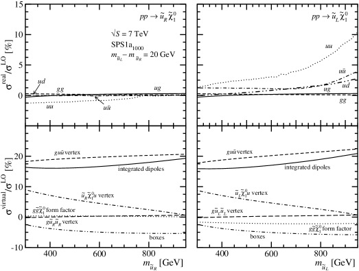
Once the on-shell diagrams are properly subtracted, we can analyze the relative numerical impact of virtual and real corrections to $\tilde{u}_{R}\,\tilde{\chi}_{1}^{0}$ and $\tilde{u}_{L}\,\tilde{\chi}_{1}^{0}$ production in Fig. 5. The different contributions are defined through dimensional regularization and (integrated) Catani-Seymour subtraction terms with $\alpha=1$ catani_seymour .

Genuine QCD effects constitute the dominant contribution. The bulk of the virtual corrections arises from gluon-mediated $qqg$ vertex corrections and the integrated dipoles. Each of them accounts for a $+20\%$ shift in the cross section for our benchmark point. The strongly suppressed gluino-mediated SUSY-QCD effects are explained by the heavy mass suppression, effectively decoupling the gluino from the theory. Correspondingly, the large vertex corrections are essentially flat as a function of the squark mass. The relative size of the integrated dipoles slightly increase with growing $m_{\tilde{q}}$ towards the gluino mass range.

Corrections to the $q$-$\tilde{q}$-$\tilde{\chi}_{1}^{0}$ vertex can reach up to $5\%$ for light squark masses. The box diagram, in turn, gives a negative contribution at the same level. Even milder is the effect from the loop-induced $g$-$\tilde{g}$-$\tilde{\chi}_{1}^{0}$ form factor, but with a different sign for the $\tilde{u}_{L}\tilde{\chi}_{1}^{0}$ or the $\tilde{u}_{R}\tilde{\chi}_{1}^{0}$ process. This again reflects the fact that they are sensitive to both the $g_{u\tilde{u}_{L}\tilde{\chi}_{1}^{0}}$ and $g_{u\tilde{u}_{R}\tilde{\chi}_{1}^{0}}$ couplings and hence the loop-induced $g$-$\tilde{g}$-$\tilde{\chi}_{1}^{0}$ form factor no longer factorizes with the Born term.

Figure 6: Profile of the renormalization and factorization scale dependence for $pp\to\tilde{u}_{R}\tilde{\chi}_{1}^{0}$. The plot traces the scale dependence following a contour in the $\mu_{R}$-$\mu_{F}$ plane covering $\mu=(0.1-10)\mu^{0}$ as shown in the left panel. We assume our benchmark parameter choice and $\sqrt{S}=7\,{\rm TeV}$.

Figure 7: Total cross section for $pp\to\tilde{u}_{R}\,\tilde{\chi}_{1}^{0}$ including the scale uncertainty. The band corresponds to a variation $\mu^{0}/2<\mu_{R,F}<2\mu^{0}$. We assume our benchmark parameter choice for all masses except for $m_{\tilde{u}_{R}}$ and show results for $\sqrt{S}=7$ TeV and 14 TeV.

II.4 Scale dependences

One of the main reasons to base LHC analyses on higher-order rate predictions is the stabilization of the dependence on the unphysical renormalization and the factorization scales. In Fig. 6 we present the cross sections as a function of the renormalization and the factorization scales varied independently. We show the cross section profile, both at leading order and at next-to-leading order, moving along a contour in the $\mu_{R}$-$\mu_{F}$ plane. The contour is defined in the left panel of Fig. 6. Individually changing one of the two scales we expect a monotonous behavior, while in the diagonal a distinct maximum appears for some processes. Again, we only show the dominant $\tilde{u}_{R}\tilde{\chi}_{1}^{0}$ channel for the modified SPS1a benchmark point with a heavy gluino.

The stabilization becomes apparent in a considerable smoothing of the $\sigma(\mu)$ slope in the entire $\mu_{R}$-$\mu_{F}$ plane. This graphical representation also indicates that the simultaneous variation of both scales would have lead to a similar uncertainty estimate, but this feature is clearly process and parameter dependent. Associated production cross sections have the feature that they are proportional to one power of $\alpha_{s}$ at leading order, which means that unlike Drell-Yan-type channels the renormalization scale dependence is visible at leading order. In contrast to QCD pair production the renormalization scale does not completely dominate the combined scale dependence, though. The NLO uncertainty band from the scale variation ranges around $(\Delta\sigma)/\sigma\lesssim 20\%$, down from up to 70% at leading order.

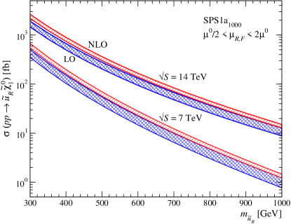
Finally, in Fig.7 we show LO and NLO cross section predictions including the scale dependence. We see that the two bands are close to overlapping for $\mu^{0}/2<\mu_{R,F}<2\mu^{0}$, i.e.  our NLO result is within the LO error estimate; on the other hand, we also see that a conservative scale variation should not be chosen any smaller. Comparing the two LHC energies we see that for 14 TeV the same number of signal events corresponds to an increase in the squark mass by at least 200 GeV.

II.5 MSSM parameter space

In Tab. 2 we survey the predictions for squark–LSP production for all SPS points. We define an inclusive $\tilde{q}\tilde{\chi}_{1}^{0}$ cross section by including the first-generation squarks, $\tilde{q}=\tilde{u}_{L},\tilde{u}_{R},\tilde{d}_{L},\tilde{d}_{R}$, but without any approximation about the individual squark masses. As we have shown, the contributions from the second generation can be safely neglected. While the set of SPS benchmark points is by no means a thorough coverage of the MSSM parameter space, this brief scan is a useful starting point and will help us understand effects from the MSSM parameter space. The whole idea of the implementation of NLO corrections in the soon-to-be public MadGolem package is of course to allow for parameter scans by any user.

	$\sqrt{S}\,[{\rm TeV}]$	$\sigma^{\text{LO}}$ [fb]	$\sigma^{\text{NLO}}$ [fb]	$K$	$K[{\tilde{u}_{L}}]$	$K[{\tilde{u}_{R}}]$	$K[{\tilde{d}_{L}}]$	$K[{\tilde{d}_{R}}]$	$m_{\tilde{u}}$	$m_{\tilde{d}}$	$m_{\tilde{g}}$	$m_{\tilde{\chi}_{1}^{0}}$
SPS1a1000	7	35.27	50.44	1.43	1.52	1.42	1.46	1.47	$\tilde{u}_{L}:561$	$\tilde{d}_{L}:568$	1000	97
	14	215.02	301.27	1.40	1.49	1.39	1.42	1.43	$\tilde{u}_{R}:549$	$\tilde{d}_{R}:545$
SPS1b	7	2.77	3.99	1.45	1.57	1.43	1.62	1.52	$\tilde{u}_{L}:872$	$\tilde{d}_{L}:878$	938	162
	14	27.21	37.46	1.38	1.48	1.36	1.52	1.43	$\tilde{u}_{R}:850$	$\tilde{d}_{R}:843$
SPS2	7	0.04	0.07	1.52	1.81	1.49	1.69	1.65	$\tilde{u}_{L}:1554$	$\tilde{d}_{L}:1559$	782	123
	14	1.21	1.64	1.36	1.45	1.34	1.46	1.45	$\tilde{u}_{R}:1554$	$\tilde{d}_{R}:1552$
SPS3	7	3.15	4.55	1.44	1.56	1.42	1.59	1.52	$\tilde{u}_{L}:854$	$\tilde{d}_{L}:860$	935	161
	14	30.20	41.59	1.38	1.49	1.36	1.50	1.43	$\tilde{u}_{R}:832$	$\tilde{d}_{R}:824$
SPS4	7	6.44	9.04	1.40	1.52	1.38	1.53	1.49	$\tilde{u}_{L}:760$	$\tilde{d}_{L}:766$	733	120
	14	52.87	71.40	1.35	1.46	1.33	1.45	1.41	$\tilde{u}_{R}:748$	$\tilde{d}_{R}:743$
SPS5	7	13.26	18.11	1.37	1.52	1.40	1.54	1.48	$\tilde{u}_{L}:675$	$\tilde{d}_{L}:678$	722	120
	14	95.81	132.29	1.38	1.50	1.37	1.49	1.43	$\tilde{u}_{R}:657$	$\tilde{d}_{R}:652$
SPS6	7	9.84	14.06	1.43	$\mathcal{O}(100)$	1.41	1.46	1.49	$\tilde{u}_{L}:670$	$\tilde{d}_{L}:676$	720	190
	14	77.08	107.03	1.39	$\mathcal{O}(100)$	1.37	1.40	1.44	$\tilde{u}_{R}:660$	$\tilde{d}_{R}:650$
SPS7	7	2.19	3.17	1.45	1.71	1.43	1.56	1.53	$\tilde{u}_{L}:896$	$\tilde{d}_{L}:904$	950	163
	14	22.36	30.80	1.38	1.61	1.36	1.46	1.43	$\tilde{u}_{R}:875$	$\tilde{d}_{R}:870$
SPS8	7	0.65	0.95	1.45	1.66	1.43	1.62	1.57	$\tilde{u}_{L}:1113$	$\tilde{d}_{L}:1122$	839	139
	14	8.73	11.79	1.35	1.43	1.34	1.44	1.42	$\tilde{u}_{R}:1077$	$\tilde{d}_{R}:1072$
SPS9	7	0.39	0.58	1.49	1.46	$\mathcal{O}(1000)$	1.51	$\mathcal{O}(1000)$	$\tilde{u}_{L}:1276$	$\tilde{d}_{L}:1279$	1872	187
	14	7.65	10.42	1.36	1.34	$\mathcal{O}(1000)$	1.38	$\mathcal{O}(1000)$	$\tilde{u}_{R}:1282$	$\tilde{d}_{R}:1289$

Table 2: Summed cross section and corresponding $K$ factors for all four first-generation squark processes $pp\to\tilde{q}\tilde{\chi}_{1}^{0}$ in different SPS benchmark scenarios. The scales are chosen at $\mu_{R,F}^{0}$. All masses are given in GeV.

First, we see that the $K$ factors are largely insensitive to the specific SPS point. This follows from the dominance of genuine QCD effects, namely the gluon-mediated $u$-$u$-$g$ vertex corrections and the real gluon emission. Changes in the squark and gluino masses do not leave a recognizable fingerprint in the relative size of the NLO corrections, which typically ranges around $40\%$. The only exception are huge corrections for $\tilde{u}_{L}$ in SPS6 and $\tilde{u}_{R},\tilde{d}_{R}$ in SPS9, which are due to essentially vanishing LO rates. To next-to-leading order rate does not factorize with the LO couplings and is instead based on additional conjugate couplings. Second, we see that the total cross sections do show a strong correlation with the SPS points; the reason is twofold: on the one hand there is kinematics, i.e.  the cross sections strongly depend on the final state masses in phase space; in addition, we see dynamics effects, where the strength of the $\tilde{\chi}_{1}^{0}q\tilde{q}$ coupling changes substantially from one scenario to another. For relative light spectra in the range $m_{\tilde{q}}\sim 500-700\,{\rm GeV}$ and $m_{\tilde{\chi}_{1}^{0}}\sim 100\,{\rm GeV}$, as is the case for SPS1a₁₀₀₀, SPS5, and SPS6, the NLO cross sections range around tens (hundreds) of femtobarns at $\sqrt{S}=7\,(14)\,{\rm TeV}$. For TeV-scale squark masses, as in SPS2, SPS8 or SPS9, the cross sections stay below the femtobarn level. The $K$ factors remain around $+40\%$. This simple pattern hardly depends on the gluino mass, since the SUSY-QCD corrections are sub-leading.

III Comparison with multi-jet merging

While experimental analyses based on NLO cross section incorporate significant improvements of the central values and the theory uncertainties, we need to ensure that this picture also includes the main distributions. From earlier studies we know that the transverse momentum and rapidity distributions of the heavy particles are relatively stable with respect to higher-order corrections prospino_squark ; thesis . Moreover, at least for the production of heavy particles QCD jet radiation should be well described by the parton shower, because the collinear approximation includes sizeable $p_{T,j}$ relative to the masses in the final state qcd_radiation . Nevertheless, we can check quantitatively how well the NLO distributions from our fixed-order MadGolem computation agree with multi-jet merging ckkw ; mlm . As a comparison and to estimate the associated theory uncertainties we use the Mlm scheme with up to two hard jets, as implemented in Madgraph. Any additional jets are well described by the parton shower qcd_radiation .

Figure 8: Squark and neutralino $p_{T}$ distributions at the LHC ($\sqrt{S}=14$ TeV) for SPS1a₁₀₀₀. We compare the merged sample with the fixed-order NLO computation. Both curves are normalized. We also show contributions to the NLO cross sections from the leading order, virtual and real parts. The latter are separated using the Catani-Seymour dipole with $\alpha=0.01$.

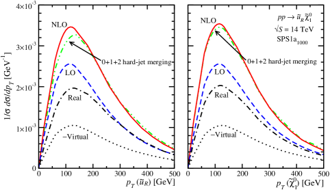
An important detail when using Catani-Seymour dipoles to compute distributions is the assignment of the unintegrated and integrated dipole contributions to phase space points. In the original paper, Ref. catani_seymour , it is spelled out that the unintegrated dipole contribution should not be counted towards their $(n+1)$-particle or in our case 3-particle phase space point, but towards the reduced 2-particle phase space. This ensures that for example the $\alpha$ dependence of the integrated and unintegrated dipoles exactly cancels not only for the total rate but also for all distributions. On the other hand, this implies that the $p_{T,j}$ distribution remains unmodified from leading order and diverges at small transverse momenta. To turn this distribution into a useful prediction we need to consistently include a parton shower lecture . Obviously, neither the leading jet distributions nor the recoiling heavy system’s distributions should be used from the fixed order computation.

In Fig. 8 we show the transverse momenta of the squark and the neutralino as computed by MadGolem and using Mlm jet merging. For the Mlm simulation we cannot subtract the on-shell singularities. However, intermediate on-shell squarks with a subsequent decay into a neutralino will produce considerably harder neutralinos through the decay phase space. Therefore we only evaluate the dominant $ug$ initial state. To the hard $ug\to\tilde{u}_{R}\tilde{\chi}_{1}^{0}$ process we add two hard and additional parton shower jets.

The normalized transverse momentum distributions agree well between the next-to-leading order and the jet merging approaches; the slightly harder result from jet merging can be attributed to additional recoil jets. This is consistent with the observation that the real emission contribution to the NLO result is slightly harder than its leading order and virtual counterparts. In contrast to Fig. 2, where we use $\alpha=1$, these distributions are computed with $\alpha=0.01$, i.e.  introducing the unintegrated subtraction term only very close to the soft and collinear poles. As a result, the virtual corrections are now smaller than the real emission contributions. Any physical observable is of course independent of the choice of $\alpha$, as discussed above.

The normalization of the merged Mlm sample is often an improvement over the leading order result, but not in a consistent quantifiable manner and to some degree dependent on the merging parameters. Therefore, it should be adjusted to the consistent NLO value.

IV Squark-neutralino channels

Figure 9: Cross sections for different squark and neutralino/chargino production channels, $pp\to\tilde{q}\tilde{\chi}_{1}^{0},\tilde{q}\tilde{\chi}_{2}^{0},\tilde{q}\tilde{\chi}_{1}^{\pm}$, as a function of the final-state neutralino/chargino mass. We show results for $\sqrt{S}=7\,{\rm TeV}$ and the modified SPS1a scenario. As in Tab. 2 we sum over all first-generation squarks. The scales are fixed to $\mu_{R,F}^{0}$.

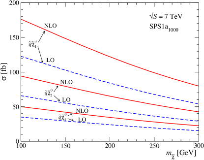
So far, we have concentrated in the associated production of a squark with the lightest neutralino. For example adding leptons to the signature we would be sensitive to the production of a squark with heavier neutralinos or charginos. On the level of the pure production these channels often have larger rate than the bino-LSP channel. In Fig. 9 we show the total cross sections for three relatively large production channels: $pp\to\tilde{q}\tilde{\chi}_{1}^{0},\tilde{q}\tilde{\chi}_{2}^{0},\tilde{q}\tilde{\chi}_{1}^{\pm}$. The cross sections for both chargino charges are summed. The differences in the total cross section for fixed neutralino/chargino masses can be traced back to the size of the $q$-$\tilde{q}$-$\tilde{\chi}$ couplings. While $g_{u\tilde{u}_{R}\tilde{\chi}_{1}^{0}}$ is the largest for the lightest neutralino, the coupling $g_{u\tilde{u}_{L}\tilde{\chi}_{2}^{0}}$ dominates for the next-to-lightest neutralino. The relative strength $(g_{u\tilde{u}_{L}\tilde{\chi}_{2}^{0}}/g_{u\tilde{u}_{R}\tilde{\chi}_{1}^{0}})^{2}\sim 1.8$ accounts for the bulk of the difference between the predicted cross sections. As before, we emphasize that our computation is based on a completely general MSSM input, encoded in a SLHA file slha . Negative mass eigenvalues for the neutralinos can be included prospino_chargino .

V Summary

We have computed the next-to-leading order QCD and SUSY-QCD corrections to the associated production of a squark with a gaugino. This channel could be responsible for the new physics signature of one hard (decay) jet and missing transverse energy. This computation is the first application of the fully automized and soon-to-be public MadGolem package. It makes no assumption about the supersymmetric mass spectrum, for example of light-flavor squarks, and relies on the SLHA interface of Madgraph. Provided its QCD counter terms are know, any new physics model with heavy strongly interacting particles can be included into MadGolem and its relevant processes generated and computed.

For the associated production of a squark and a neutralino we find that NLO corrections due to gluon exchange and radiation dominate and lead to a typical correction around $+40\%$. Gluinos only play an appreciable role when they are very light, which in the light of recent ATLAS and CMS measurements is becoming increasingly unlikely. The NLO transverse momentum distributions we have compared with a Mlm merged computation and find good agreement for the heavy particles produced. To avoid any dependence on merging parameters, the total cross section should be based on the fixed-order NLO computation.

For associated production processes like the one considered here, it is crucial to implement a consistent and stable on-shell subtraction scheme separating associated production from QCD-mediated pair production. The automization of this subtraction in the Prospino scheme is part of MadGolem.

MadGolem: Automizing NLO predictions for new physics

MadGolem completely automates the calculation of cross sections and the generation of parton-level events at NLO for arbitrary $2\to 2$ processes in a generic new physics framework. Its highly modular structure we illustrate in Fig. 10. For the generation of all tree-level Feynman diagrams and amplitudes we use Madgraph madgraph , which also provides user interfaces and the basic code structure. The one-loop Feynman diagrams we generate with Qgraf qgraf and a subsequent set of specialized routines:

1. First, we translate the Qgraf output into a code suitable for symbolic calculation languages. The structures describing the Feynman diagrams and the corresponding Feynman rules we rewrite as algebraic expressions, keeping track of external wave functions, vertex couplings and internal propagators, color factors, Lorentz structure, and the overall sign from external fermion fields. With this modification MadGolem can cope with genuine features of new physics processes, such as Majorana fermions.

2. Then, we map the analytical evaluation of the color, helicity and tensor structures onto partial amplitudes, i.e.  a basis of color, helicity and tensor structures based on the spinor-helicity formalism.

3. In addition, we apply an analytical reduction to scalar loop integrals, based on a modified Passarino-Veltman reduction scheme implemented in Golem golem .

4. Finally, we combine the results with the ultraviolet counter terms (which are also generated automatically). The final output for the virtual corrections we return both as analytical Maple and numerical Fortran90 code.

Figure 10: Modular structure of MadGolem.

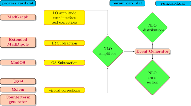
To compute complete NLO rates MadGolem uses dedicated modules for the different types of divergences appearing in NLO calculations. To remove infrared divergences from real and virtual gluon emission we resort to the Catani-Seymour dipole subtraction catani_seymour . Our automatic dipole generation is a modified and extended version of MadDipole maddipole , now including all massive Standard Model and supersymmetric dipoles. All integrated dipoles explicitly retain the dependence on the phase space coverage of the subtraction term $\alpha$ alpha . Intermediate on-shell divergences we remove following the Prospino scheme described in Sec. II.3 prospino_onshell . Its local subtraction terms we generate automatically. The ultraviolet renormalization counter terms we generate with Madgraph amplitude. They are expressed in terms of two-point functions which are supplied in a separate library. The current library supports QCD corrections for arbitrary $2\ \to 2$ processes in the Standard Model and the MSSM and can easily be generalized to other new physics models.

MadGolem does not require the user to interfere with the computation of NLO cross section and parton-level events from the basic input. The model and the process are specified through Madgraph input cards. Options like multi-particle notation are supported together with additional specifications that allow us, for instance, to separate QCD from SUSY-QCD contributions or retain subsets of one-loop contributions.

We have performed exhaustive checks to ensure the reliability of MadGolem. Total NLO cross sections we have tested both in the SM and the MSSM and covering numerous initial/final states, interactions, and topologies. Cancellation of all divergences and gauge invariance of the overall result have been confirmed numerically and analytically. The finite renormalized one-loop amplitudes we have compared with FeynArts, FormCalc and LoopTools results feynarts . Particular attention we have paid to numerical stability and convergence of our Catani-Seymour dipoles and the on-shell subtraction. Finally, we have checked our final results with the literature (e.g.  $e^{+}e^{-}\to\tilde{q}^{*}\tilde{q}$ eesquark ) as well as with Prospino prospino-slepton and MadFks madfks (e.g.  $pp\to\tilde{\ell}^{*}\tilde{\ell}$).

References

- (1) D. E. Morrissey, T. Plehn and T. M. P. Tait, arXiv:0912.3259 [hep-ph].
- (2) ATLAS Collaboration, ATLAS-CONF-2010-065; CMS Collaboration, arXiv:1101.1628 [hep-ex]; D. S. M. Alves, E. Izaguirre and J. G. Wacker, arXiv:1008.0407 [hep-ph].
- (3) C. Englert, T. Plehn, P. Schichtel, S. Schumann, Phys. Rev. D83, 095009 (2011).
- (4) P. Bechtle, K. Desch, M. Uhlenbrock, P. Wienemann, Eur. Phys. J. C66, 215-259 (2010); E. Turlay, R. Lafaye, T. Plehn, M. Rauch, D. Zerwas, J. Phys. G G38, 035003 (2011).
- (5) E. L. Berger, M. Klasen, T. M. P. Tait, Phys. Rev. D62, 095014 (2000) [Erratum-ibid. D67, 099901 (2003)]; M. Spira, arXiv:hep-ph/0211145; T. Plehn, [arXiv:hep-ph/0410063].
- (6) V. D. Barger, K. Hagiwara, J. Woodside, W. -Y. Keung, Phys. Rev. Lett. 53, 641 (1984); R. M. Barnett, H. E. Haber, G. L. Kane, Phys. Rev. Lett. 54, 1983 (1985).
- (7) L. Vacavant [ ATLAS and CMS Collaborations ], Eur. Phys. J. C33, S924-S926 (2004). G. F. Giudice, T. Plehn, A. Strumia, Nucl. Phys. B706, 455-483 (2005); E. Gerwick, D. Litim, T. Plehn, Phys. Rev. D83, 084048 (2011).
- (8) T. Plehn, C. Weydert, PoS CHARGED2010, 026 (2010). [arXiv:1012.3761 [hep-ph]].
- (9) T. Plehn, arXiv:hep-ph/9809319.
- (10) P. Z. Skands, B. C. Allanach, H. Baer et al., JHEP 0407 (2004) 036.
- (11) J. Pumplin, D. R. Stump, J. Huston, H. L. Lai, P. Nadolsky and W. K. Tung, JHEP 0207, 012 (2002).
- (12) T. Plehn, D. Rainwater, P. Z. Skands, Phys. Lett. B645 (2007) 217-221; T. Plehn and T. M. P. Tait, J. Phys. G 36 (2009) 075001; J. Alwall, S. de Visscher, F. Maltoni, JHEP 0902 (2009) 017.
- (13) S. Catani, F. Krauss, R. Kuhn et al., JHEP 0111 (2001) 063.
- (14) M. L. Mangano, M. Moretti and R. Pittau, Nucl. Phys. B 632 (2002) 343.
- (15) B. C. Allanach, S. Grab and H. E. Haber, JHEP 1101, 138 (2011) [arXiv:1010.4261 [hep-ph]].
- (16) S. P. Martin and M. T. Vaughn, Phys. Lett. B 318, 331 (1993).
- (17) W. Beenakker, M. Klasen, M. Krämer, T. Plehn, M. Spira and P. M. Zerwas, Phys. Rev. Lett. 83, 3780 (1999) [Erratum-ibid. 100, 029901 (2008)].
- (18) W. Beenakker, R. Höpker, M. Spira and P. M. Zerwas, Phys. Rev. Lett. 74, 2905 (1995); W. Beenakker, R. Höpker, M. Spira and P. M. Zerwas, Nucl. Phys. B 492 (1997) 51.
- (19) S. Berge, W. Hollik, W. M. Mösle and D. Wackeroth, Phys. Rev. D 76, 034016 (2007).
- (20) B. C. Allanach et al., in Proc. of the APS/DPF/DPB Summer Study on the Future of Particle Physics (Snowmass 2001) ed. N. Graf, Eur. Phys. J. C 25, 113 (2002).
- (21) W. Beenakker, R. Höpker, T. Plehn, P. M. Zerwas, Z. Phys. C75, 349-356 (1997).
- (22) see e.g. S. Frixione, E. Laenen, P. Motylinski et al., JHEP 0807, 029 (2008).
- (23) J. Alwall et al., JHEP 0709, 028 (2007).
- (24) H. Murayama, I. Watanabe, K. Hagiwara, prepring KEK-91-11.
- (25) P. Nogueira, J. Comp. Phys. 105, 279 (1993).
- (26) T. Binoth, J. P. Guillet, G. Heinrich, E. Pilon and T. Reiter, Comput. Phys. Commun. 180, 2317 (2009); G. Cullen, J. P. Guillet, G. Heinrich, T. Kleinschmidt, E. Pilon, T. Reiter and M. Rodgers, arXiv:1101.5595 [hep-ph].
- (27) S. Catani and M. H. Seymour, Nucl. Phys. B 485, 291 (1997) [Erratum-ibid. B 510, 503 (1998)]; S. Catani, S. Dittmaier, M. H. Seymour and Z. Trocsanyi, Nucl. Phys. B 627, 189 (2002).
- (28) S. Frixione, Z. Kunszt and A. Signer, Nucl. Phys. B 467, 399 (1996). Z. Nagy and Z. Trocsanyi, Phys. Rev. D 59, 014020 (1999) [Erratum-ibid. D 62, 099902 (2000)].
- (29) R. Frederix, T. Gehrmann and N. Greiner, JHEP 0809, 122 (2008); and JHEP 1006, 086 (2010).
- (30) A. Signer, D. Stöckinger, Phys. Lett. B626, 127-138 (2005). and Nucl. Phys. B808, 88-120 (2009).
- (31) K. Hikasa, Y. Nakamura, Z. Phys. C70, 139-144 (1996); A. Djouadi, W. Hollik, C. Jünger, Phys. Rev. D55, 6975-6985 (1997); A. Alves, O. Eboli, T. Plehn, Phys. Lett. B558, 165-172 (2003).
- (32) T. Hahn, Comput. Phys. Commun. 140, 418 (2001); T. Hahn and C. Schappacher, Comput. Phys. Commun. 143, 54 (2002); T. Hahn and M. Pérez-Victoria, Comput. Phys. Commun. 118, 153 (1999).
- (33) M. Drees and K. Hikasa, Phys. Lett. B 252, 127 (1990).
- (34) W. Beenakker, M. Klasen, M. Krämer, T. Plehn, M. Spira and P. M. Zerwas, Phys. Rev. Lett. 83, 3780 (1999) [Erratum-ibid. 100, 029901 (2008)].
- (35) R. Frederix, S. Frixione, F. Maltoni and T. Stelzer, JHEP 0910, 003 (2009).
- (36) for a pedagogical introduction see e.g. T. Plehn, [arXiv:0910.4182 [hep-ph]].