An index for regular expression queries:
Design and implementation

Abstract

The like regular expression predicate has been part of the SQL standard since at least 1989. However, despite its popularity and wide usage, database vendors provide only limited indexing support for regular expression queries which almost always require a full table scan.

In this paper we propose a rigorous and robust approach for providing indexing support for regular expression queries. Our approach consists of formulating the indexing problem as a combinatorial optimization problem. We begin with a database, abstracted as a collection of strings. From this data set we generate a query workload. The input to the optimization problem is the database and the workload. The output is a set of multigrams (substrings) which can be used as keys to records which satisfy the query workload. The multigrams can then be integrated with the data structure (like B+ trees) to provide indexing support for the queries. We provide a deterministic and a randomized approximation algorithm (with provable guarantees) to solve the optimization problem. Extensive experiments on synthetic data sets demonstrate that our approach is accurate and efficient.

We also present a case study on PROSITE patterns - which are complex regular expression signatures for classes of proteins. Again, we are able to demonstrate the utility of our indexing approach in terms of accuracy and efficiency. Thus, perhaps for the first time, there is a robust and practical indexing mechanism for an important class of database queries.

1 Introduction

Consider a simple database query:

SELECT doc.id FROM doc where doc.text LIKE ’%har%’

Current database systems have to carry out a full table scan to answer the above query. For large databases (like collections of documents) this can be extremely time consuming rendering the use of regular expression queries almost infeasible.

In the above query, the query poser may be searching for documents which contain the text share or shard or something else. To speed up query processing, the database designer could potentially create an index where the keys are multigrams (substrings) which point to all records which contain that multigram - the posting list of the multigram. In this instance, there are several choices that could be made. For example, the index algorithm may decide to select the multigram har or ha or ar or nothing at all.

To process the query, the query engine will determine if there is any of the text fragments in the regular expression query belong to the key set of the index. If so, then the index will be scanned to retrieve the posting list for that multigram. The query engine then will apply the regular expression template on each record of the posting list and select those that are matched. The query processing framework is shown in Figure  1.

In Figure 1, the diagram shows the simplified process flow view of our regular expression query framework. It can be seen that the index is made up of two components: (1) multigrams - index keys; (2) posting lists - database record filter list. When user submits a query request, the regular expression will be firstly submitted to the regular expression rule engine in step one. At the same time, the query will be broken down into query keys in step two. Then, these query keys will be used to match the multigrams as well as the posting list in step three, four and five. Then, it will generate a candidate database record set to answer the regular expression query. In step six, the candidate database records are passed to the regular expression rule engine, which has already incorporated with the regular expression of interest in step one, and finally produces the query answer in step seven.

If no index is employed to answer the query request, step two to step five will be ignored, and the entire database will be passed to the regular expression engine to process in step six. Generally, this is named as “full table scan” in the database community.

The key challenge is in deciding what to index. For example, the advantage of indexing har over ha is efficiency: the database records which contain the text har is a subset of those which contain ha resulting in lower IO cost for queries which contain har. The disadvantage is that fewer queries are likely to use this key compared to ha. Thus the index designer has to (i) control the size of the index by bounding the maximum number of multigrams that can be indexed, (ii) balance the trade-off between the likelihood of a multigram being used by a query and the size of its posting list.

1. We present a novel algorithm which selects the multigrams to index. Note that the number of possible multigrams is infinite. Our approach is to cast the multigram selection problem as an integer program and then use a linear programming relaxation, followed by rounding to select the multigrams.

2. Using the above algorithm, we have implemented a fully functional regular expression query framework on top of a commercial database.

3. We have carried out extensive experiments to test for the accuracy, efficiency and robustness of the regular expression querying framework.

4. We present a novel case study using protein data where regular expression patterns are used routinely to classify families of proteins.

The rest of the paper is as follows. In Section 2 we report on related work. Section 3 formalizes the index selection problem in an integer programming framework and presents a small example to illustrate how the algorithm selects the multigrams that are indexed. Section 4 presents the Linear Programming Multigram Selection (LPMS) algorithm and the related theory. In Section 5 we report on the extensive set of experiments to test the query framework. We also present a case study in a real application. We conclude in Section 6 with a summary and directions for future research. Appendix 1 describes all the data sets that were created and used for the experiments.

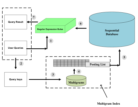
Figure 1: A generic indexed query framework consists of $7$ steps. Whereas, if no indexes are employed, steps $2$ to $5$ will be skipped

2 Related Work

Traditionally a regular expression query is processed by constructing a non-deterministic finite automata (NFA) which recognizes the language defined by the regular expression pattern [15, 19, 11]. The entire database is processed one character at a time resulting in $O(mn)$ time and $O(m^{2})$ space, where $m$ and $n$ are the size of the regular expression and database respectively.

The two most commonly indexes which have been currently using in both database systems are B+trees [3, 10] and bitmaps [6]. Both of them are designed to support exact pattern matching rather than regular expression querying. Therefore, some database vendor tailor these indexes to support regular expression query, such as: full text indexing in PostgreSQL, and function-based index in Oracle. However, their application is criticized as quite restricted.

From an indexing perspective, tries and suffix trees [4, 22, 13, 24, 9, 16], which are lexicographical ordered trees, can be used to support regular expression queries. However, the major weakness of tries and related structures like suffix-trees is that the size of the index is often much larger than the size of the database that is being indexed.

Basically, its structure is categorized as a lexicographical ordered tree. The height of a trie, $H(n)$, represents the longest path from the root to a leaf node where $n$ is the database size. For a random and uniform distributed string database, $H(n)=$ $2log_{2}(n)+o(log_{2}(n))$ [18]. Therefore, we can see that trie is feasible to achieve sub-linear query run time. In fact, it is reported that in the worse case, the number of nodes (i.e. query space) could be $O(n^{2})$ [2]. In other words, it indicates that trie improves the query time at the expense of the query space. This may result in creating the thorny issues such as memory trashing and bottleneck especially in conditions where the database size is considerably large.

In order to reduce the number of node while sustaining trie’s performance, Weiner [24] transformed Trie to the first suffix tree structure, that the index is built by processing the database string from right to left which takes $O(nH(n))$ time. Later, Ukkonen [22] developed a left-to-right built algorithm that maintains a suffix tree which takes $O(n)$ time. In later research, this suffix tree was later augmented with suffix link [16] to form a directed acyclic word graph which leads to an algorithm for the construction of the automata.

In another stream of research, inverted files [25] and q-grams [21, 5, 17] are two designs which support information retrieval and informatics. However, both are not suitable for regular expression queries because they rely on a predefined list of words.

More recently, a relatively different research strand has been developed to support regular expression querying. The initial work in this area was carried out by Cho and Rajgopalan - the authors who denote their index as FREE multigram index [7].

The principle of the FREE model is direct and straightforward. The objective is to select the minimal useful multigram set. A multigrams is considered ‘useful’ as long as the number of data records containing the multigrams that are smaller than a threshold (namely selectivity or support). Otherwise it is considered ‘useless’. The FREE algorithm consists of a series of iterations starting with a single character multigram ($k=1$), whereas in each iteration, all minimal useful multigrams of length $k$ are then selected. The remaining are considered ‘useless’ and form the the prefix-seeds of the multigrams in the next iteration. The process is continually repeated until there is no ‘useless’ multigram is left. The algorithm is designed so that the set of useful multigrams selected is prefix-free.

The key insight of the FREE algorithm is that the size of the prefix-free multigram index is always bounded above by the database size.

This is an important property that all regular expression indexes should enforce. Since FREE selects low support multigrams, queries which use FREE always take less time than queries which employ a full table scan. However the disadvantage of FREE is that it does not take any query workload into account and thus many queries are unlikely to utilize the index.

To overcome the weakness of FREE, Hore et. al. [12] (in a 2004 CIKM paper) proposed a multigram selection algorithm called BEST which takes both the database a query workload into consideration. In the BEST algorithm, each multigram is associated with a cost factor $c$ (equivalent to the support) and at the same time associated with the query set by a benefit factor, $b$. The benefit of the multigram is equal to the number of records that can be pruned when utilized by a query. The ratio of $\frac{b}{c}$ forms the utility value which is defined as the objective function to optimize both the index efficiency and query hit rate at the same time.

Hore formalizes the multigram selection problem as an instance of the Budgeted Maximum Coverage (BMC) [14] problem. Specifically the cover set forms the ‘Budgeted’ part while the utility of the index is captured in the ‘Coverage’ component. The main principle of the BEST algorithm is to select multigrams which increase the index hit rate so more queries can utilize the algorithm. However, a major weakness of the BEST algorithm is that it neither scales to large datasets nor large query workloads because it uses a cartesian product of query workload and database as the search space.

Our approach is inspired by both FREE and BEST. Like the BEST algorithm we take both the database and query workload into consideration but unlike BEST we generate a representative workload from the database. The advantage of having both a database and workload is that we can formalize the problem in a combinatorial optimization framework. We also formalize the problem in a way which ensures that the set of multigrams selected are prefix-free. Thus we are able to bound the size of the index and guarantee that the running time of a query using the index will be less than the full database scan.

3 The index selection problem

In this section we will use the integer programming framework to formalize the index selection problem. We will also provide a small example which explains how the integer programming solution returns multigrams which can then be indexed. In this section we will assume that the query workload is given. In practice we generate a representative workload from the database. In Section 4 we will show how the integer program can be relaxed to return the solutions in an efficient manner.

3.1 Problem Definition

To recall we are given a database, abstracted as a collection of strings, and a set of regular expression queries $Q$. Our objective is to select a set of multigrams which will be used as keys of an index for efficiently answering the queries in $Q$.

The index will be used to retrieve a set of candidate records from the database which may satisfy the query. After the candidate records are selected, the actual regular expression matching is done in memory to select the exact set of records which satisfy the query.

For the purpose of indexing we will treat each query $q$ as a set of multigrams $M_{q}$. Let $\bar{M}_{q}$ be the set $M_{q}$ and all the substrings of length at least one which appear within each multigram in $M_{q}$.

Let $G=\bigcup_{q\in Q}\bar{M}_{q}$ be the universe of candidate multigrams. It is from $G$ that we will select a subset $G_{I}$ which will form the index.

Example 1

Suppose the set $Q$ consists of a single query $q=(ex).\{1,3\}(ess)$. Then $M_{q}=\{ex,ess\}$ and $\bar{M}_{q}=\{ex,es,ss,ess\}$

To formalize the index selection problem as an integer program (IP) we need to define (i) integer variables ($x$), (ii) the constraints ($A,b$) and (iii) the objective function ($c$) and set up the problem as

$$\begin{array}[]{lll}\mbox{minimize}&\sum\limits_{g\in G}c_{g}x_{g}&\\[8.61108pt] \mbox{subject to}&Ax\geq b&\\[8.61108pt] &x\in\{0,1\}\end{array}$$ (1)

For each multigram $g$ in $G$ we associate an integer binary variable $x_{g}\in\{0,1\}$. The variable $x_{g}$ will be set to one if the multigram $g$ is selected to be part of the index. To formalize the constraints we will construct a $|Q|\times|G|$ matrix A such that

$$A_{i,j}=\left\{\begin{array}[]{ll}s(g_{j})&\mbox{if }g_{j}\in\bar{M}_{q_{i}};\\ 0&\mbox{otherwise}.\end{array}\right\}$$ (2)

Here $s(g)$ is the support or the number of rows in the database in which the multigram $g$ appears at least once. It is through the definition of $A$ that the integer program captures the characteristics of the underlying database. We also need to define the $|Q|$ dimensional vector $b$ which defines the right hand side of the system $Ax\geq b$. Here we define

$$\begin{array}[]{l}b_{i}=\min\limits_{g\in\bar{M}_{q_{i}}}s(g)\;\;\forall i\end{array}$$ (3)

The definition of $b_{i}$ can be interpreted as follows. Each row of $A$ represents a query. The row constraint captures the smallest number of database records that must be returned if the query will use the index. This is captured with multigram $g$ with the smallest support contained in the expanded query $\bar{M}_{q}$.

We now define the objective function which is typically of the form

$$\begin{array}[]{l}\sum\limits_{g\in G}c_{g}x_{g}\end{array}$$ (4)

The objective should capture the trade-off between the coverage of a multigram and it is support in a database. By coverage we mean that one multigram can be used by several queries. On the other hand if the support of this multigram is high (relative to the size of the database) then the index is not necessarily useful as a full table scan may only be slightly less efficient. For example suppose the objective is to select multigrams to index text documents. Then selecting the word “the” as an index is not very efficient as most documents in the database will be returned as candidates. In the language of information retrieval the choice of multigrams need to balance the trade-off between precision versus recall.

Since we want to cast the IP as a minimization problem we want to select multigrams which have low support and at the same time we want the selected multigram to be used by as many queries as possible. Thus we define

$$\begin{array}[]{l}c_{g}=\frac{s(g)}{|g|\sum\limits_{q\in Q}\imath(g\in\bar{M}_{q})}\end{array}$$ (5)

where $\imath(g\in\bar{M}_{q})$ is an indicator function. Thus the numerator of $c_{g}$ is the support of the multigram $g$ and we want multigrams with small support (making the index more efficient) and at the same time we want to select multigrams with high coverage so fewer multigrams need to selected to form the index.

Theorem 1

The solution vector $x$ returned by the integer program represents a set of multigrams which form a prefix-free set.

Proof 3.2.

The proof will be by contradiction. Suppose $x$ does not return a prefix-free set. Let $x_{u}$ and $x_{v}$ represent multigrams $u$ and $v$ such that $u$ is a prefix of $v$ and therefore

1. $s(u)\geq s(v)$.

2. If $v\in\bar{M}_{q}$ then $u\in\bar{M}_{q}$ and

3. $\frac{1}{|u|}\geq\frac{1}{|v|}$

Thus $c_{u}\geq c_{v}$. Now if construct a new vector $x^{\prime}$ such

$$x^{\prime}(g)=\left\{\begin{array}[]{ll}x(g)&\mbox{ if}g\neq u\\ 0&\mbox{ otherwise }\end{array}\right.$$

Then $\sum_{g\in G}c_{g}x^{\prime}_{g}<\sum_{g\in G}c_{g}x_{g}$. Furthermore by construction of the constraint matrix $Ax^{\prime}\geq b$. This violates the minimality of $x$. Thus the solution returned by the integer program must be prefix-free.

The importance of having a prefix-free index set has been noted (and proved) before by Cho and Rajgoplan [7]. Essentially the prefix-freeness guarantees that the size of the index (as measured by the number of pointers into the database) is bounded by the size of the database. More formally (and in our notation)

Theorem 3.3.

If $x$ is the vector returned by the integer program and $|R|$ is the size of the underlying database then

$$\sum_{\{g:x_{g}=1\}}s(g)\leq|R|$$

The importance of Theorem 1 and 2 cannot be underestimated. For the first time we have a principled way of selecting a set of multigrams to index. The definition of the problem gives us prefix-freeness. As a result the constraint on the size of the index is now endogenous to the problem as opposed to providing an exogenous (budget) constraint as in the BEST method [12].

3.2 An example of index selection with integer programming

In this section we will walk through a simple example to illustrate how the integer programming approach can be used for multigram selection.

Table 1 shows a simplified word database. Table 2 shows two typical regular expression queries. For instance, the first query looks for the words in the word database that contains the substrings, ‘ex’ or ‘pr’, followed by any substring of length between 1 and 3 and then immediately followed by the substrings, ‘eed’ or ‘ess’. Since the regular expression is composed of an ‘or’ predicate, all the or-ing elements within the regular expression must be uniquely identified to avoid ambiguity. In column two of Table 2, we show that the first regular expression query is broken down into four non-or regular expression queries.

The word database consists of 62 multigrams with length ranging from two to four Only 14 multigrams are relevant to the two regular expression queries. In table 3, we lists out all the multigrams in the word database that relevant for $Q$. From equation 2, 3 & 5, we can calculate matrix $A$ and vector $c$ and $b$.

Table 1: The word database $R$ contains 8 records made up of the multigram set $\bar{M}_{2,q}$ as elaborated in table 3

$r_{1}$	‘succeed’	$r_{4}$	‘recede’	$r_{7}$	‘succession’
$r_{2}$	‘proceed’	$r_{5}$	‘secession	$r_{8}$	‘excess’
$r_{3}$	‘precede’	$r_{6}$	‘exceed’

Table 2: Query set $Q$ contains 2 regular expression queries with 14 (out of 64) multigrams

Regular Expression	$M_{q}$
(ex)$|$(pr).{1,3}(eed)$|$(ess)	$q_{1}$:(ex).{1,3}(ess)
	$q_{2}$:(ex).{1,3}(eed)
	$q_{3}$:(pr).{1,3}(ess)
	$q_{4}$:(ex).{1,3}(eed)
(pr)$|$(re).{1,2}(cede)	$q_{5}$:(pr).{1,2}(cede)

Table 3: The multigram set $\bar{M}_{2,q}$ for $R$ & $Q$ contains 64 multigrams with length ranging from 2 to 4

	$g_{j}$,$s(g_{j})$		$g_{j}$,$s(g_{j})$		$g_{j}$,$s(g_{j})$
$g_{1}$	‘ex’, 2	$g_{6}$	‘ed’, 5	$g_{11}$	‘ced’,2
$g_{2}$	‘es’, 3	$g_{7}$	‘eed’, 3	$g_{12}$	‘ede’,2
$g_{3}$	‘ss’, 3	$g_{8}$	‘pr’, 2	$g_{13}$	‘cede’,2
$g_{4}$	‘ess’, 3	$g_{9}$	‘ce’, 8	$g_{14}$	‘re’,2
$g_{5}$	‘ee’, 3	$g_{10}$	‘de’, 2	$g_{15}$

Therefore, $\large A$ =

$$\left(\begin{array}[]{cccccccccccccc}2&3&3&3&0&0&0&0&0&0&0&0&0&0\\ 2&0&0&0&3&5&3&0&0&0&0&0&0&0\\ 0&3&3&3&0&0&0&2&0&0&0&0&0&0\\ 0&0&0&0&3&5&3&2&0&0&0&0&0&0\\ 0&0&0&0&0&5&0&2&8&2&2&2&2&0\\ 0&0&0&0&0&5&0&0&8&2&2&2&2&2\\ \end{array}\right)$$

, $\large c$ = (1 1.5 1.5 1 1.5 2.5 1 1 4 1 0.6 0.6 0.5 1) and $\large b$ = (2 2 2 2 2)’.

When the problem instance $(A,b,c)$ are fed into an integer program solver, the returned solution vector $\large x$ = (1 0 0 0 0 0 0 1 0 0 0 0 1 0)’ or $g_{1}$, $g_{8}$ & $g_{13}$. As a result, ‘ex’, ‘pr’, ‘cede’ are the optimal set of multigram selected.

4 A Linear Programming Relaxation

In the previous section we have presented a model for the multigram selection problem based on integer programming. We proved that the the resulting multigrams form a prefix-free set.

However theoretically the general integer program problem is NP-Hard and even in practice algorithms for IP programs require exponential time for most instances. This is because unlike linear programming problems where convexity of the problem can be exploited (local optima are global optima), for integer programming the full lattice of feasible points has to be explored  [23].

A common approach to get around the complexity of integer programs is relax them to linear programs which can then be solved efficiently (in polynomial time). The solution of the linear program provides a natural lower bound (for minimization problems) for the integer program. The linear program fractional solution then needs to be converted to an integer solution. There are two approaches for carrying out the conversion. The first approach is to select a deterministic threshold and use that to round the solutions. The second approach is to interpret the solution vector (typically between 0 and 1) as probabilities and carry out a randomized rounding.

For the rest of the paper, the solution of multigram selection problem obtained using the integer program will be referred as IPMS (Integer Program Multigram Selection). Similarly those obtained from deterministic and randomized rounding of the linear program will will form the basis of the LPMS-D and LPMS-R algorithms respectively.

4.1 The LP Relaxation

The LP relaxation of the integer program is

$$\begin{array}[]{lll}\mbox{minimize}&\sum\limits_{g\in G}c_{g}x_{g}&\\[8.61108pt] \mbox{subject to}&Ax\geq b&\\[8.61108pt] &0\leq x\leq 1\end{array}$$ (6)

Clearly if the optimal solution of the integer program is denoted as $OPT_{I}$ and the solution of the linear program is denoted as $OPT_{LP}$ then $OPT_{LP}\leq OPT_{I}$.

Now the solution vector returned by the linear program is fractional and so we need to convert the fractional solution into an integer solution.

Theorem 4.4.

Let $s_{\max}$ and $s_{\min}$ be the multigram in $G$ with the largest and smallest non-zero support respectively. Furthermore let $m^{\ast}=\max_{q\in Q}|\bar{M_{q}}|$. If $x_{l}$ is the solution of the relaxed linear program and we convert it to an integer solution by rounding up all elements in $x_{l}$ which are greater than $\frac{s_{\min}}{s_{\max}m^{\ast}}$ then the rounded solution is a feasible solution of the integer program and achieves a constant approximation to the original integer program

Proof 4.5.

All we have to show is that if all elements of $x_{l}$ are less than $\frac{s_{\min}}{s_{\max}m^{\ast}}$ then $x_{l}$ is not a feasible solution of the linear program.

Now this is true because for each row $i$ of $Ax\geq b$ there are only $m^{\ast}$ non-zero entries in each row sum and therefore

$$\sum\limits_{j}a_{ij}x_{j} <s_{\max}m^{\ast}\frac{s_{\min}}{s_{\max}m^{\ast}}=s_{\min}$$

This contradicts the feasibility of $x_{l}$ (as $Ax\geq b$). Thus by rounding all terms based on the threshold we not only get a feasible solution but the value of the cost function goes up by at most $\frac{s_{\max}m^{\ast}}{s_{\min}}$
Furthermore the approximation is obtained by noting that

$$OPT_{LP}\leq OPT_{IP}\leq\frac{s_{\max}m^{\ast}}{s_{\min}}OPT_{LP}$$ (7)

Therefore,

$$x_{l}^{D}=\left\{\begin{array}[]{ll}1&\mbox{if }x_{l}>s_{\max}m^{\ast}\frac{s_{\min}}{s_{\max}m^{\ast}}\\[8.61108pt] 0&\mbox{otherwise}\end{array}\right\}$$ (8)

The above theorem will be used as a basis for designing a deterministic rounding algorithm LPMS-D.

4.2 LP Relaxation - Randomized Rounding

While the deterministic rounding algorithm gives an approximate and feasible solution, the approximation bound is quite loose. A more practical solution is to use randomized rounding by interpreting the values of the linear program solution as probabilities. Thus each component of $x_{l}$ is treated like a probability. The cost function can be treated as a random variable and it is easy to show that the expected value of the cost function is equal to value of the linear program.

4.3 Prefix free enforcement

While LP relaxation and rounding allows us to overcome the exponential runtime complexity of integer programs, it does not guarantee that the resulting multigram set is a prefix-free. The resulting size of the index may not be bounded by the database size. In order to overcome this shortcoming, we enforce the prefix-free constraint by proposing an iterative algorithm- LPMS.

Algorithm 1 outlines the LPMS multigram prefix-free selection process. The expandSet starts with an element “.”. Then each element in expandSet is expanded by appending each character from the alphabet set, $\Sigma$, which will form the childrenSet. Then all query keys contained in the query set, $Q$, are consolidated to generate the $\bar{M}_{q}$ set. After this any multigrams in the childrenSet that are not present in the $\bar{M}_{q}$ set will be removed. Then the refined childrenSet and set $Q$ will form the input to an LP solver to produce the linear programming solution, $x$. Finally, $x$ is relaxed by applying either deterministic or randomized rounding. Those multigrams with its associated x value equals to “1” will be selected as the multigram and saved in a set $G$. All unselected multigrams will then replace the current expandSet. The process will be repeated until the expandSet is empty, i.e., all the multigrams are selected.

Input: string database (R), query set (Q), alphabet set ($\Sigma$)

Output: Multigram index (G)

expandSet = {.};

repeat

      For each multigram in the expandSet, append a member in $\Sigma$ and save to the childrenSet;

      Remove all multigram g $\in$ childrenSet if g $\notin$ $\bar{M}_{k,q}$ $\forall$ $k$;

      Populate matrix A, b, c of the LP model using formulae (2), (3) and (5) respectively;

      Apply LPMS-D or LPMS-R to find the vector x;

      Move all multigrams whose associated value in the vector x $=1$ to G;

      Those multigrams remaining will become the expandSet;

     

      until (expandSet = {});

ALGORITHM 1 LPMS multigram selection algorithm

5 Experiments Roadmap

We have carried out extensive experiments to test our approach for accuracy, efficiency and robustness. The experiment roadmap is shown in Table  4. There are total of five experiments which includes one case study on a real protein data set. For each of the experiment we generate a different synthetic data set to vary conditions appropriate for that particular experiment. The details of data generation are given in Appendix 1.

5.1 Experiment 1 - Accuracy and Performance

In this experiment we measure accuracy and performance of our proposed LPMS-D and LPMS-R and compare it with the FREE approach. We use recall as the measure of accuracy which captures the percentage of queries which use the index. For performance we measure precision which effectively measure what percentage of candidate records are actually satisfied by a query in the workload. We created several data sets by varying the standard deviation of the support distribution of the multigrams. The details of data generation are in Appendix 1.

The results are summarized in Figure  2 and 2. In Figure 2 we measure the precision and recall of the LPMS-R, LPMS-D and FREE as a function of the different data sets. As expected (since we proved it) we get a recall of one for LPMS-D. However note that the recall of LPMS-R is also very high -greater than 0.98 in all cases. Thus even after randomized rounding our approach is still able to satisfy most of the constraints of the integer program. Not surprisingly the recall of the FREE approach is very low. This is because the FREE method uses a set of prefix-free multigrams of low support as the basis of the index. The FREE approach does not use the query workload for designing the index.

When it comes to precision, the story is the opposite. The precision of FREE is greater than that of LPMS-R which is greater than LPMS-D. Again, FREE indexes multigrams with small support so when a multigram is selected by a query it is bound to have selected only a few candidate records making the precision high.

A more interesting result is to compare the precision of LPMS-D and LPMS-R which is shown in Figure 2. Here the X-axis represents the query-id’s ranked by their precision on LPMS-R. Thus the query with the highest precision using LPMS-R is on the left. For each of the query we also calculated the precision of LPMS-D. The results clearly show that for almost all instances, the precision of LPMS-R is higher than that of LPMS-D.

The results of Figure 2 allow us to conclude that LPMS-R is highly accurate (with recall almost equal to that of LPMS-D) and also very efficient (as precision is a measure of efficieny).

Table 4: Road map of the five experiments performed to evaluate the LPMS multigram index

Expt	Objective and Description	Data Type	Data Set Description	Metric	Results
1	Compare accuracy and performance of LPMS-R,	Synthetic	Data sets with varying	Precision	Fig 2 and 2
	LPMS-D, RDB and and FREE [7]		support distribution of	and
			multigrams	Recall
2	Scalability of LPMS-R and LPMS-D	Synthetic	Data sets with varing	Build time	Figure 3(a) and 3(b)
			data and query workload	and Query
			size	time
3	Quality of LPMS-R relaxation vis-a-vis	Synthetic	Same as Experiment 2	Size of	Table 5
	optimal Integer Program and			index
	BEST [12]			(posting list)
4	Robustness of index as query workload change	Synthetic	Data sets with varying	Precision	Table 6
			alphabet size	and
				Recall
5	Case Study on Prosite protein patterns using	Real	Protein database[1]	Precision	Figure 4 and
	LPMS-D		and Prosite pattern	and
			query[20]	Recall

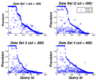
Figure 2: Experiment 1: (a) The recall of LPMS-D > LPMS-R $>>$ FREE; the precision of FREE > LPMS-R > LPMS-D. (b) For almost all queries the precision of LPMS-R is higher than LPMS-D. This suggests that LPMS-R is both highly accurate and yet more efficient than LPMS-D. Note that the recall of FREE is very low making it ineligible as a serious candidate for indexing.

5.2 Experiment 2 - Scalability

In this experiment we measure the execution time of the componets of Algorithm 1 (LPMS-R). Algorithm 1 has three distinct components: (i) multigram generation (ii) model construction and (iii) model solver - which invokes a call to a linear programming engine.

The multigram generation time (MGT) is the time required to generate all the candidate multigrams and also calculate their support value. The model construction time (MCT) is the time required to populate the matrix $A$, the constraint vector $b$ and the cost function $c$.

The execution time is measured as a function of varying data size and query workload. In the first set of experiments, the data set size are varied between 20K and 100K while keeping the query workload size to 1000. In the second set, the data set size is fixed but the query workload varies between 90K and 500K. Details data set and query workload generation is described in Appendix 1.

FIgure 3(a) shows the running time for MGT, the MCT and overall index construction processing as a function of increasing database size. The MGT scales linearly with database size, the MCT remains nearly constant and the overall time also scales linearly. The MCT remains constant as the size of the matrix $A$ and $b$ is dependent on the size of the query workload which is kept constant.

Figure 3(b), shows the running time as a function of increasing query workload. As expected the MGT is constant (as the database size is kept constant). The MCT scales linearly with query workload size and the overall time increases in a super-linear fashion. This is not surprising because the overall time includes the time to invoke and execute the linear programming engine. Further refinements, like using a primal-dual approach instead of invoking a linear solver (like simplex) may help reduce the overall time.

However, we can conclude that the current approach scales nearly linearly with both database size and query workload size thus making the proposed approach feasible and practical.

5.3 Experiment 3 - Optimality

In Experiment 3 we measure the divergence from “optimality” of LPMS-R and LPMS-D. The Integer Programming Multigram Selection (IPMS) gives the optimal solution but is only feasible and practical for small data sets. Thus on small data sets we can experimentally compare how far the solution returned from LPMS is from IPMS. We also compare our approach against the BEST algorithm explained earlier [12]. The BEST algorithm associates a benefit value with each multigram. We sort the multigrams by benefit value and select the top 100,110,120,130,140,150, 200 and 250 multigrams. The top 250 multigrams result in a hit rate of 100%, i.e., all the queries in the workload use the index. Again, the data set which consists of 2000 records and 100 queries is described in Appendix 1.

The optimality results comparing LPMS-R, IPMS and BEST are shown in Table  5. The IPMS selects multigrams whose posting size is remarkably small - just 106! LPMS-R selects multigrams with a posting size of 2773. This implies an average precision of 0.304. The posting list of the BEST algorithm start at 6,774 and by the time the top 250 multigrams are selected, the size of the posting list has increased to 17,107. Clearly LPMS-R is far superior to the BEST approach.

Index	# correct	Precision	Posting	Prefix
type	query	Mean/Std	size	Free
IPMS	100	1/0	106	Y
LPMS-R	99	0.304/0.435	2,773	Y
B-100	91	0.097/0.28	6,744	N
B-110	94	0.067/0.23	7,396	N
B-120	95	0.056/0.21	8,110	N
B-130	97	0.036/0.17	8,814	N
B-140	98	0.025/0.13	9,513	N
B-150	99	0.016/0.099	10,156	N
B-200	99	0.014/0.099	13,578	N
B-250	100	0.004/0.002	17,107	N

Table 5: Experiment 3: On small data sets we can exactly solve for the integer programming solution. The optimal posting list size is 106 and LPMS-R returns a list of size of 2,773. The size of the posting list of BEST, for similar levels of accuracy, is greater than 10,000. Posting list is a measure of index efficiency.

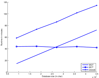
(a) The overall build time for LPMS-R scales linearly with database size

(b) The overall build time for LPMS-R scales super-linearly with query workload size

Figure 3: Experiment 2: Scalability of the LPMS-R construction time as a function of (a) database size; (b) query size. Near-linear scalability suggests that LPMS is a practical method for index generation.

5.4 Experiment 4: Robustness

The objective of this experiment is to measure to what degree the index is useful for queries which were not explictly used for constructing the index.

We created four different data sets Rob01-Rob04, composed from the alphabet ’A-D’, ’A-H’, ’A-L’ and ’A-P’ respectively. Each data set contains 5,000 records. The details of the data set are in Appendix 1.

We next defined a query pattern with a key length bounded between three and eight. For example, the following sample query consists of three query keys and two gap constraints.

“(HFBFD)(.0,9)(AEHDCEAG)(.0,39)(CCCGDAAE)”

Using this query pattern, three sample query sets are generated from the $10\%$, $30\%$ and $50\%$ sample of Rob01, Rob02, Rob03 and Rob04. Then, LPMS-R and LPMS-D indexes are constructed using each sample query set and each data set. This will create twenty-four LPMS multigram indexes. For example, index ‘LPMS-R-10’ in row two and column 3 of table 6 is constructed on the data set Rob03, based on the $10\%$ sample query set.

For querying we generated five independent test query sets, each from the $2\%$ sample of Rob01, Rob02, Rob03 and Rob04. This will create twenty independent test query sets. These test query sets are tested against the corresponding LPMS-R and LPMS-D indexes.

Table 6 reports the test results. It shows that the recall of all sixty sets of LPMS-D query are equal to $1$ except in a few exceptional occasions. In the LPMS-R query, the recall decreases as the alphabet size increases. Then, the recall improves as its corresponding index sample size increases.

On the other hand, the precision of the LPMS-R queries are not consistent. However, the precision of the LPMS-D queries consistently improve as the sample size increases.

These results clearly show that the performance of the LPMS-D multigram index is depending on the sample size. In other words, for a given query pattern, if the sample database size is large enough, the LPMS-D multigram index is capable to support arbitrary query and produce accurate result. In addition, by further increasing the sample size, the precision will be further improved. This clearly shows that the LPMS-D is robust.

Table 6: Experiment 4: The recall values of both LPMS-R and LPMS-D on test sets on several data sets. See text for explanation. High recall values suggests that both LPMS-R and LPMS-D are robust against query perturbations.

	Rob01	Rob02	Rob03	Rob04
LPMS-R-10	1	0.78	0.63	0.45
LPMS-R-30	0.98	0.82	0.72	0.61
LPMS-R-50	1	0.95	0.81	0.58
LPMS-D-10	1	1	0.99	0.98
LPMS-D-30	1	1	1	1
LPMS-D-50	1	1	1	1

5.5 Case Study: PROSITE Patterns

So far the previous four experiments have focused on studying the performance of the LPMS in a controlled fashion. In this section, the objective is to apply the LPMS multigram on a real data and contemporary application.

We selected 100K protein sequences from the PFAM-A protein database [1]. Each sequence is composed of 20 distinct amino acids (alphabet) with length ranging from 4 to 2750. The query set is made up of $100$ Prosite signatures [20], which are downloaded from the PDB [8]. Each Prosite signature is a regular expression defining a protein class.

Figure 4 shows the data flow of the LPMS-D multigram index Prosite-Protein application. Step 1 through Step 5 on the right of figure 4 shows how the LPMS-D multigram index is constructed. While step A to step E on the left shows how the LPMS-D multigram is used to process a Prosite query.

For example, consider the Ribosomal protein S18 (PS000057) from the Prosite pattern [20].

“[IVRLP]-[DYN]-[YLF]-x(2,3)-…[RHG]-[LIVMASR]"

The S18 protein pattern is first translated into regular expression, and is passed to the ‘POSIX Reverse Matching engine’ in step A.

“[IVRLP][DYN][YLF].{2,3}…[RHG][LIVMASR]"

Here multigrams that match the regular expression are retrieved from index database in step B and C. For example, ‘IDY’, ‘YYX’, … etc. In step D, the posting list will generate a list of candidate protein database records that will potentially match the query S18. Finally, in step E and F, the regular expression rule matching is performed, which will produce the query result.

Figure 4: Data flow diagram for the Full POSIX Prosite-Protein application. The data flow step 1 to step 5 on the right show the LPMS-D Multigram index construction process. The data flow step A to step E on the left show the LPMS-D Multigram index query process.

One hundred Prosite queries were tested against the protein database with and without the LPMS-D index. The recall of this test was equal to $1$, which demonstrates that the LPMS-D index is $100\%$ accurate.

Furthermore, we repeat the experiment by restricting the multigram set allowable in the index construction to be of size at least three. As expected the recall was lower and equal to $0.56$. This suggests that by restricting the size of the universe of allowed multigrams we can balance the trade-off between accuracy and efficiency.

6 Summary and Conclusion

While modern database management systems support forms of regular expression querying, they do not provide any indexing support for such queries. Thus, a regular expression query requires a full database scan to find the matching records. This is a severe limitation as the database size will continue to increase and applications for such queries (e.g., bioinformatics) proliferate.

In this paper, we have proposed a robust, scalable and efficient approach to design an index for such queries. The heart of our approach is to model the multigram selection problem as an integer program (IP) and show that the approximate solutions of the IP have many of the properties we desire: accuracy robustness and efficiency. Extensive set of experiments on both synthetic and real datasets demonstrate our claimed contributions.

For future work we will replace the current linear programming solver by using a primal-dual approach which will make the approach handle very large query workloads. Furthermore we will test our approach in other application domains including intrusion detection systems.

7 Appendix 1: Data Sets

7.1 Experiment 1

We generated five data sets using the English alphabet by varying the support distribution of the multigrams. The different support distribution was created as a function of a Normal distribution by varying the standard deviation between 100 and 500. The support distribution of the multigrams is shown in Figure 5.

Based on the support distribution of the multigrams, synthetic databases were reverse engineered which contained multigrams of prescribed support. Finally, using a query pattern consisting of three query keys and two gap constraints, the query workload was generated. The size of the five databases ranged from 380 - 420K and the size of the query workload ranged between 227 and 248.

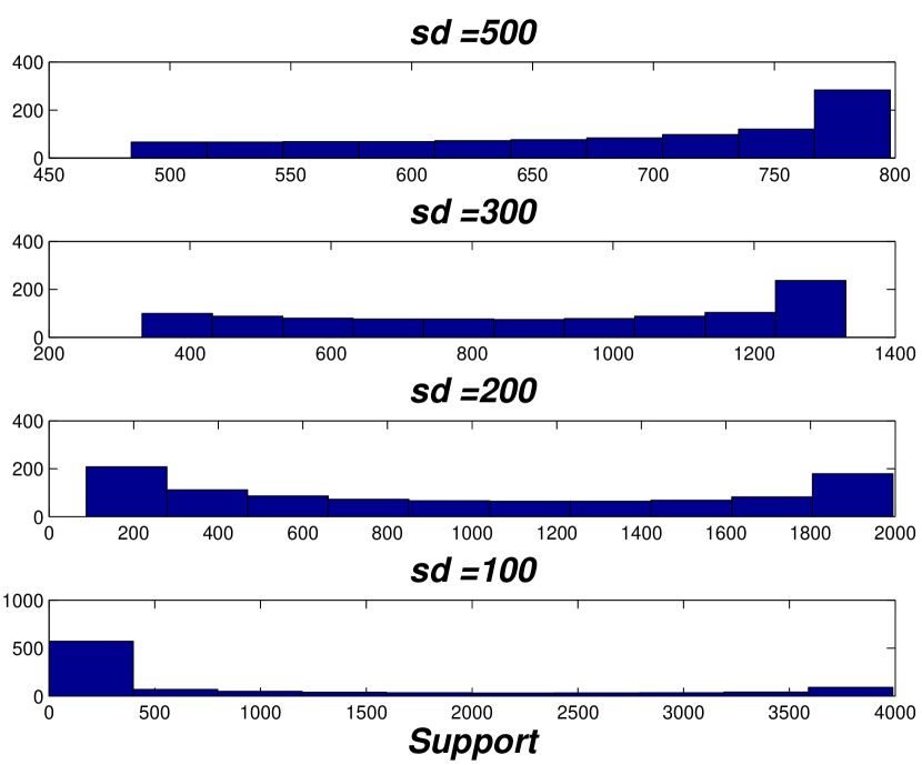
Figure 5: Experiment 1: The support distribution of multigrams was generated and both database and query workload were reverse engineered to approximately match the multigram distribution

7.2 Experiment 2

Five data sets were synthetically generated using a random number generator on the English alphabet. Then a database sample of $10\%$ was taken from each of the data set to generate a query work load. No distribution (of multigrams) was prescribed as in Experiment 1. The query workload was fixed (to 1000) and then database size was varied and then the database size was fixed and the query workload was between between $90K$ and $500K$. However, the size of the data sets are varied by increasing changing the data set size, while the query work load is kept to $1,000$.

7.3 Experiment 3

To test for optimality we sampled a data set generated from Experiment 2. The data set size was reduced to $20K$ and the query workload to $100$. This was necessary as integer programming solutions require exponential time in most instances.

7.4 Experiment 4

Data set for the robustness experiment was again synthetically generated on the English alphabet. Specifically, data sets Rob01, Rob02, Rob03 and Rob04 are composed of the alphabet ‘A-D’, ‘A-H’, ‘A-L’ and ‘A-P’ respectively. Each data set contains $5,000$ records with their total database size and mean record sets are volumetrically similar.

Next, in experiment 4, three database samples, $10\%$, $30\%$ and $50\%$ are taken from the four Rob data sets which form the basis of twelve LPMS-D and twelve LPMS-R multigram indexes.

References

- [1] Pfam-a database. http://pfam.sanger.ac.uk, 2008(accessed 2011).
- [2] R. Baeza-Yates and G. Gonnet. Fast text searching for regular expressions or automaton searching on tries. Journal of the ACM, 43(6):915–936, 1996.
- [3] R. Bayer and C. McCreight. Organization and maintenance of large ordered indexes. ACTA Informatica, pages 173–189, 1972.
- [4] R. Braindais. File searching using vaiable keys. In AFIPS Western JCC, pages 295–298, 1959.
- [5] S. Burkhardt, A. Crauser, P. Ferragina, H. Lenhof, E. Rivals, and M. Vingron. q-gram based database searching using a suffix array. In:RECOMB99, ACM, New York, pages 77–83, 1999.
- [6] C. Chan and Y. E. Ioannidis. Bitmap index design and evaluation. ACM SIGMOD, pages 355–366, 1998.
- [7] J. Cho and S. Rajagopalan. A fast regular expression indexing engine. Proceedings 18th International Conference on Data Engineering, 2002.
- [8] S. CJA, C. L, de Castro E, L.-G. PS, B. V, B. A, and H. N. Prosite, a protein domain database for functional characterization and annotation. Nucleic Acids Res. 38(Database issue)161-6, 2010.
- [9] M. Farach, P. Ferragina, and S. Muthukrishnan. Overcoming the memory bottleneck in suffix tree construction. 39th Annual Symposium on Foundations of Computer Science, 1998.
- [10] P. Ferragina and R. Grossi. The string b-tree: a new data structure for string search in external memory and its applications. JACM, pages 46(2):236–280, 1999.
- [11] J. E. Hopcroft, R. Motwani, and J. D. Ullman. Introduction to Automata Theory, Language, and Computation. Addison-Wesley, 2001.
- [12] B. Hore, H. Hacigumus, and B. Lyer. Indexing text data under space constraints. CIKM 04 November 8-13, Washington, DC, USA, 2004.
- [13] E. Hunt, M. Atkinson, and R. Irving. Database indexing for large dna and protein sequence collections. The VLDB Journal, 11:256–271, 2002.
- [14] S. Khuller, A. Moss, and J. Naor. The budgeted maximum coverage problem. IPL, 70:29–45, 1999.
- [15] D. Knuth, J. Morris, and V. Pratt. Fast pattern matching in strings. Comput. Sci. Rep. STAN-CS-74-440, Stanford, Calif, 1974.
- [16] E. M. McCreight. A space economical suffix tree construction algorithm. Journal of ACM, 23, No. 2:262–272, 1976.
- [17] G. Navarro, E. Sutinen, and J. Tarhio. Indexing text with approximate q-grams. In:CPM2000, Lecture Notes in Computer Science, Springer, Berlin Heidelberg New York, 1848:350–365, 2000.
- [18] M. Regnier. On the average height of trees in digital search and dynamic hashing. Inf. Proc. Letters, 13:64–66, 1981.
- [19] R. Rivest. On the worst-case behavior of string-searching algorithms. SIAM J on Computing, 6:669–674, 1977.
- [20] C. J. A. Sigrist, L. Cerutti, N. Hulo, A. Gattiker, and L. Falquet. Prosite: A documented database using patterns and profiles as motif descriptors. Henry Stewart Publications, 3:265–274, September 2002.
- [21] E. Ukkonen. Approximate string matching with q-grams and maximal matches. Theoret Comput Sci, pages 92(1):191–212, 1992.
- [22] E. Ukkonen. On-line construction of suffix trees. Algorithmica, 14:249–260, 1995.
- [23] V. V. Vazirani. Approximation Algorithms. Springer, 2003.
- [24] P. Weiner. Linear pattern matching algorithm. IEEE 14th Ann. Symp. on Switching and Automata Theory, pages 1–11, 1973.
- [25] I. Witten, A. Moffat, and T. Bell. Managing gigabytes: compression and indexing documents and images. Morgan Kaufamann, San Francisco, Calif., USA, 1999.