Electronic Liquid Crystalline Phases in a Spin-Orbit Coupled Two-Dimensional Electron Gas

Abstract

We argue that the ground state of a two-dimensional electron gas with Rashba spin-orbit coupling realizes one of several possible liquid crystalline or Wigner crystalline phases in the low-density limit, even for short-range repulsive electron-electron interactions (which decay with distance with a power larger than 2). Depending on specifics of the interactions, preferred ground-states include an anisotropic Wigner crystal with an increasingly anisotropic unit cell as the density decreases, a striped or electron smectic phase, and a ferromagnetic phase which strongly breaks the lattice point-group symmetry, i.e. exhibits nematic order. Melting of the anisotropic Wigner crystal or the smectic phase by thermal or quantum fluctuations gives rise to a non-magnetic nematic phase which preserves time-reversal symmetry.

I introduction

Enhancing the role of electron-electron interactions relative to that of the kinetic energy often leads to interesting many-body effects. Electron crystallization is an extreme example of this phenomenon. At low densities, where electrons are far apart and the kinetic energy cost of localization is low, Coulomb interactions dominate and the electrons form an ordered state, known as a Wigner crystalWigner (1934).

The nature of the crystallized electronic state has been intensely investigated through Quantum Monte Carlo (QMC) calculations Tanatar and Ceperley (1989); Drummond and Needs (2009). These calculations support the existence of the crystalline phase, though the density at which they find crystallization is typically significantly lower than what heuristic arguments would suggest. The Wigner crystal has also been sought experimentally. Despite difficulties associated with reaching the ultra-low density regime where crystallization is expected, evidence that the Wigner crystal phase may have been realized has been reported for experiments on ever-cleaner samples of two-dimensional electron gases (2DEGs) in semiconductor quantum wellsYoon et al. (1999).

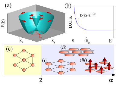
Figure 1: (a) Dispersion of a particle with Rashba SOC. The minimum of the dispersion occurs on a ring in $k$ space, marked by a red circle. The red arrows show the spin polarization of the different Bloch states. (b) Density of states as a function of energy, corresponding to the dispersion shown in (a). Near the band bottom, the density of states diverges as $\rho(E)\sim(E)^{-1/2}$. (c) Schematic phase diagram in the low-density limit with repulsive electron-electron interactions which decay at long distances as $V\sim r^{-\alpha}$. For $\alpha\leq 2$, the ground state is an isotropic Wigner crystal (i.e. it preserves a discrete rotational symmetry, C_n with $n>2$). For $\alpha>2$, states with a further broken rotational symmetry are favored. (i) represents an anisotropic Wigner crystal with a unit cell which becomes parametrically anisotropic in the low–density limit. (ii) and (iii) represent snapshots of a smectic state and a ferromagnetic nematic liquid state, respectively.

In this paper, we study the low density limit of the 2DEG system with Rashba spin-orbit coupling (SOC), which is present whenever the 2DEG lacks inversion symmetryRas . This is the case, for example, when the 2DEG is confined in an asymmetric quantum well, or if it is formed at the surface of a three-dimensional material. As shown in Fig.1a, the resulting dispersion relation has an extended (highly degenerate) minimum which forms a ring in momentum space. The low-energy density of states exhibits a divergent van Hove singularity, $\rho(\varepsilon)\sim\varepsilon^{-1/2}$, akin to the behavior of a one-dimensional system (see Fig. 1b). This is in striking contrast to the usual behavior $\rho(\varepsilon)\sim{\rm const}$, familiar for two-dimensional systems without spin-orbit coupling. Thus the Rashba SOC greatly enhances the role of interactions relative to that of kinetic energy in the low-density limit.

For a system with Coulomb interactions, $V(r)\sim 1/r$, the ground state at low densities is a Wigner crystal, just as for a 2DEG without spin orbit coupling. Remarkably, however, we find that with Rashba SOC, broken symmetry states appear to be favored over the uniform Fermi liquid (UFL) state even for short-range interactions, $V(r)\sim 1/r^{\alpha}$ with $\alpha>2$. (In particular, note that the Coulomb interaction screened by a metallic gate is described by $\alpha=3$.) The instability in this case occurs at an electron density $n$ for which the Fermi energy is smaller than an energy scale set by the SOC.

We have investigated candidate ordered states by constructing variational wave-functions, determining the patterns of broken symmetry which minimize their variational energies, and then comparing the energy to that of the UFL. We consider the following types of broken symmetry states: 1) Wigner crystalline (WC) states, i.e. insulating states with only discrete translational symmetry corresponding to one electron per unit cell, allowing for various possible crystal structures corresponding to different patterns of rotation symmetry breaking; 2) an electron smectic state which breaks translational symmetry in only one direction, and can be viewed as a partially melted version of an anisotropic WC; 3) a ferromagnetic nematic state which preserves translation symmetry, but breaks time reversal symmetry and rotational symmetry - this state is invariant under time reversal followed by a rotation by $\pi$ around the symmetry axis. Note that we refer to a WC as anisotropic when only a discrete 2-fold rotation symmetry (C₂) remains unbroken. In the limit of low density, each of these ordered states has parametrically lower energy (in powers of the density $n$) than the UFL. This strongly suggests that the UFL is unstable at low densities. In contrast, the energy balance between different broken symmetry phases is more delicate, and may well depend on long-distance fluctuational effects that are not well captured by variational wavefunctions; we will return to this point in the final section of the paper.

The nature of the low-density instability of the UFL, and the origin of the strong tendency of the system to a nematic pattern of rotation symmetry breaking (whether or not it is accompanied by other patterns of symmetry breaking) can be most easily seen by studying candidate WC wavefunctions. A schematic version of the resulting WC phase diagram is shown in Fig. 1c as a function of the exponent $\alpha$. For $\alpha>2$ (short-range interactions), the unit cell of the Wigner crystal becomes increasingly anisotropic, with an aspect ratio that diverges in the low-density limit. This unusual behavior can be traced back to the form of the single-particle dispersion, Fig.1a, which is strongly anisotropic in the directions perpendicular and tangential to the ring-like minimum.

A complimentary view can be obtained by considering a ferromagnetic state. Because of the Rashba SOC, the orientation of the magnetization vector (which is always in-plane) necessarily defines a preferred nematic axis - any ferromagnetic state must necessarily be nematic, although a non-magnetic nematic phase is possible. For example, a magnetic moment in the y direction implies a special role for the point $\vec{k}_{0}$ in Fig. 1a, which defines the point on the ring of minimum dispersion with the largest possible value of $k_{x}$. At low density, the resulting Fermi surface forms an ellipse encircling this special point. As in the usual Stoner theory of ferromagnetism, spin polarization lowers the interaction energy via the Pauli-exclusion principle, which helps electrons to avoid each other at short distances. However, the cost in kinetic energy is parametrically smaller than in a conventional FL, owing to the divergent density of states. The variational energy we find for the ferromagnetic nematic state differs from that of the anisotropic crystal only by a numerical constant for $2<\alpha\leq 3$, so it is not possible, on the basis of the present considerations, to confidently determine which (if either) is the preferred ground state. For $\alpha>3$, the ferromagnetic nematic state has parametrically lower energy than the anisotropic WC, suggesting that it is a better candidate ground state. The scaling of the ground state energy as a function of the electron density for each type of state considered in this paper is listed in Table 1.

Table 1: Scaling of the ground state energy per particle as a function of the electron density $n$ in the low density limit, for the various candidate ground states considered in this paper: the nematic ferromagnetic (FM) state, the anisotropic Wigner crystal (AWC), and the smectic. For $\alpha<2$, the isotropic Wigner crystal always has the lowest energy.

state	$2<\alpha\leq 3$	$3<\alpha\leq 4$	$4<\alpha$
nematic FM	$n^{2\left(1-\frac{1}{\alpha}\right)}$	$n^{2\left(1-\frac{1}{\alpha}\right)}$	$n^{\frac{3}{2}}$
AWC or smectic	$n^{2\left(1-\frac{1}{\alpha}\right)}$	$n^{\frac{4}{3}}$	$n^{\frac{4}{3}}$

This paper is organized as follows. The model is described in Sec. II. In Sec. III, we explain the basic physics leading to anisotropic Wigner crystal formation. We analyze three cases: contact interactions, extended short-range interactions (which fall off with distance with a power which is larger than 2), and long-range interactions. Considerations related to the magnetic structure of the Wigner crystal phase are discussed in Sec. IV. In Sec. V we discuss melting the Wigner crystal partially to obtain a smectic state. In Sec. VI we discuss the ferromagnetic nematic state. Sec. VII presents a proposed schematic phase phase diagram for a 2DEG with SOC and screened Coulomb interactions. In Sec. VIII we discuss possible realizations in electronic and atomic systems. Appendix A presents the solution of a single Rashba particle in a box problem, which is crucial for the arguments regarding the anisotropic Wigner crystal and the smectic phases, and Appendix B presents the details of the Hartree-Fock analysis of the ferromagnetic nematic state.

II Model

We consider a 2DEG with Rashba SOC and repulsive electron-electron interactions, described by the Hamiltonian (in units with $\hbar=1$)

$$H = \sum_{j}\left\{\frac{1}{2m}\left[-\nabla_{j}^{2}-\frac{2k_{0}}{i}(\nabla_{j}\times{\hat{z}})\cdot\vec{\sigma}_{j}\right]+E_{0}\right\}$$ (1)

$$+ \frac{1}{2}\sum_{l\neq j}V(|\vec{r}_{l}-\vec{r}_{j}|)\text{.}$$

Here, $m$ is the electronic effective mass, $k_{0}$ is a parameter that characterizes the strength of the SOC, $E_{0}\equiv k_{0}^{2}/(2m)$, $\vec{\sigma}_{j}$ is the vector of Pauli matrices which act on the spin of electron $j$, and $V(|\vec{r}|)$ is the (repulsive) electron–electron interaction potential. The Hamiltonian (1) is invariant under translations, under rotations around the $z$ axis, and under mirror reflections about the $x$ and $y$ axes, $M_{x}$ and $M_{y}$, but not under inversion $\vec{r}\rightarrow-\vec{r}$.

Below we consider cases in which, at large inter-particle separation $r$, the interaction potential decays as a power law:

$$V\left(|\vec{r}|\right)\sim\frac{V_{0}}{r^{\alpha}}\text{.}$$ (2)

We distinguish between long-range and short-range interactions, which are characterized by $\alpha\leq 2$ and $\alpha>2$, respectively. The bare Coulomb interaction is described by $\alpha=1$, while screening can lead to $\alpha>1$. In particular, screening due to a nearby metallic gate top gate leads to $\alpha=3$.

In the absence of interactions, $V(|\vec{r}|)=0$, Eq. (1) yields the single-particle dispersion law (see Fig. 1a):

$$E(\vec{k})=\frac{1}{2m}\left(k^{2}\pm 2k_{0}k\right)+E_{0},$$ (3)

where $\vec{k}$ is the electron momentum ($\hbar=1$), and $k=|\vec{k}|$. The minimum kinetic energy occurs for any value of momentum falling on a ring of radius $k=k_{0}$, with a minimal value of $E=0$. The corresponding density of states, shown in Fig. 1b, is given by

$$D\left(E\right)=\left\{\begin{array}[]{ccl}\frac{m}{\pi}\sqrt{\frac{\left|E_{0}\right|}{E}}&&(E<E_{0}),\\ \frac{m}{\pi}&&(E>E_{0}).\end{array}\right.$$ (4)

For $E>E_{0}$, the density of states is independent of energy, just as for a usual 2DEG without spin-orbit coupling. However, for $E\rightarrow 0$, the density of states diverges as $1/\sqrt{E}$. Because this divergence will play a crucial role in the analysis below, we comment briefly on its origin. The divergence comes from the fact that the minimum of kinetic energy is infinitely degenerate, occurring everywhere on a ring in momentum space, rather than at a single point or finite set of points. In the presence of crystalline anisotropy (which manifests itself through corrections to the effective mass approximation in real materials), the divergence is cut off near the band bottom and the density of states goes to a constant. However, as long as $k_{0}a/\pi\ll 1$, where $a$ is the lattice constant (i.e. as long as the spin-orbit coupling is weak), the crystal field anisotropy terms are small and Eq. (4) provides a good approximation down to energies of order $|E_{0}|(k_{0}a)^{2}$ above the band bottom.

III Wigner crystal

III.1 Instability of the Fermi liquid state

We begin by considering the stability of the uniform (Fermi liquid) state. According to Eq. (4), at low densities, the Fermi energy $\varepsilon_{F}$ is

$$\varepsilon_{F}=\frac{\pi^{2}n^{2}}{4m^{2}\left|E_{0}\right|}\text{,}$$ (5)

where $n$ is the density of electrons per unit area. Thus, the kinetic energy per particle in the homogeneous state is

$$\bar{\varepsilon}_{\text{kin}}=\frac{1}{n}\int_{0}^{\varepsilon_{F}}\varepsilon D\left(\varepsilon\right)d\varepsilon=\frac{\pi^{2}n^{2}}{12m^{2}\left|E_{0}\right|}\text{.}$$ (6)

The potential energy per particle, on the other hand, is

$$\bar{\varepsilon}_{\text{pot}}=\frac{1}{2n\Omega}\int d\vec{r}d\vec{r}^{\prime}V\left(\vec{r}-\vec{r}^{\prime}\right)\langle n(\vec{r})n(\vec{r}^{\prime})\rangle\text{,}$$ (7)

where $\Omega$ is the total area of the system, $n(\vec{r})$ is the local density at position $\vec{r}$, and $\langle\cdots\rangle$ denotes averaging in the uniform (Fermi gas) state. In the low–density limit, for short-range interactions ($\alpha>2$ in Eq. 2), $\bar{\varepsilon}_{\text{pot}}\propto n$. For long-range interactions, the right hand side of Eq. (7) diverges. Here a neutralizing background must be taken into account, leading to $\bar{\varepsilon}_{\text{pot}}\propto n^{\alpha/2}$. We see that in all cases, in the low-density limit, $\bar{\varepsilon}_{\text{pot}}\gg\bar{\varepsilon}_{\text{kin}}$, suggesting that the uniform state is unstable to forming some sort of order. One possibility is that at asymptotically low densities, the ground state is a Wigner crystal, as in a 2DEG with no SOC. Note, however, that here, in the presence of Rashba SOC, this instability occurs even for short-range interactions.

III.2 Contact interactions

For simplicity, we begin by considering the case of the shortest range interactions: repulsive “contact” interactions. We start with a variational wavefunction which minimizes the interaction energy, taking each electron to be confined to a rectangular box of dimensions $L_{x}\times L_{y}$, with different boxes non-overlapping. This is a zero energy eigenstate of the potential energy operator. In order for the boxes to tile the plane, $L_{x}$ and $L_{y}$ are constrained by the condition

$$L_{x}L_{y}=\frac{1}{n}.$$ (8)

Thus, we have a single variational parameter, the aspect ratio $\eta\equiv L_{x}/L_{y}$, which we use to minimize the kinetic energy of the trial state. The kinetic energy per particle in the variational state is given by the ground state energy of a single particle in a box with Rashba SOC. This problem is investigated, both analytically and numerically, in Appendix A. Surprisingly, unlike the case with no SOC, the ground state energy in the low–density limit is minimal for $\eta\neq 1$. In the $\eta\gg 1$ limit, we find the following expression for the ground state energy as a function of $\eta$ and $n$:com (a)

$$\varepsilon\left(n,\eta\right)=\frac{n}{2m}\left(A\eta^{-1}+\frac{Bn}{k_{0}^{2}}\eta^{2}\right),$$ (9)

where $A$ and $B$ are numbers of order unity, see Eq. (39) in Appendix A. Minimizing Eq. (9) with respect to $\eta$, we find that the optimal aspect ratio $\eta^{\star}$ scales as

$$\eta^{\star}\sim\left(n/k_{0}^{2}\right)^{-\frac{1}{3}},$$ (10)

and the ground state energy per particle scales as

$$\varepsilon^{\star}\left(\eta^{\star}\right)\sim\left|E_{0}\right|\left(n/k_{0}^{2}\right)^{\frac{4}{3}}\text{.}$$ (11)

Therefore, in the low–density limit, we get that the energy per particle of this anisotropic Wigner crystal state is parametrically lower than that of the uniform state, which scales as $n$. Note that, consistent with our assumptions, the optimal aspect ratio of the unit cell in the Wigner crystal becomes parametrically large at low densities.

The fact that the kinetic energy is minimal for an anisotropic box can be understood as follows. Suppose that the ground state wavefunction is a superposition of plane waves with wavevectors close to some wavevector $\vec{k}^{\star}$ of length $k_{0}$, for which the dispersion (3) is minimal. Near $\vec{k}^{\star}$, the dispersion is quadratic in the radial direction, while it is anomalously flat (quartic) in the transverse direction. Therefore confinement in the direction perpendicular to $\vec{k}^{\star}$ is less costly than confinement parallel to $\vec{k}^{\star}$, and the optimal aspect ratio is such that the box is long in the direction of $\vec{k}^{\star}$, and short in the transverse direction.

III.3 Extended short-range interactions

We now turn to the case of extended, short–range interactions, which corresponds to $2<\alpha<\infty$. We show that in this case, as in the case of contact interactions, the Wigner crystal state is extremely anisotropic in the low–density limit.

In the case of extended interactions, the potential energy in the Wigner crystal phase cannot be neglected. To estimate the potential energy, we consider the same variational wave function as before, in which the particles are localized in an array of non-overlapping $L_{x}\times L_{y}$ boxes. To estimate the potential energy, we will replace the wavefunction of each particle by a constant, such that the density is uniform, $n=1/(L_{x}L_{y})$; the parametric dependence of the energy on $n$ and $\eta$ should not depend on this assumption. Let us focus on the anisotropic limit, $L_{x}\gg L_{y}$, assuming that this is the optimal configuration. The interaction energy of a given particle with all the other particles is

$$\bar{\varepsilon}_{\text{v}}\left(n,\eta\right) \approx 2(U_{1}+U_{2}),$$ (12)

where $U_{1}$ and $U_{2}$ are given by

$$U_{1} =\frac{1}{L_{x}^{2}L_{y}^{2}}\int_{0}^{L_{x}}dx\int_{0}^{L_{y}}dy\int_{-\infty}^{\infty}dx^{\prime}\int_{L_{y}}^{\infty}dy^{\prime}\frac{V_{0}}{\left[(x-x^{\prime})^{2}+(y-y^{\prime})^{2}\right]^{\alpha/2}}=V_{0}n^{\frac{\alpha}{2}}\eta^{\frac{\alpha}{2}-1}C_{1}$$ (13)

and

$$U_{2} =\frac{1}{L_{x}^{2}L_{y}^{2}}\int_{0}^{L_{x}}dx\int_{0}^{L_{y}}dy\int_{L_{x}}^{\infty}dx^{\prime}\int_{0}^{L_{y}}dy^{\prime}\frac{V_{0}}{\left[(x-x^{\prime})^{2}+(y-y^{\prime})^{2}\right]^{\alpha/2}}=V_{0}n^{\frac{\alpha}{2}}\eta^{\frac{\alpha}{2}-2}\left[C_{2}+O\left(\eta^{2-\alpha}\right)\right].$$ (14)

$C_{1}$ and $C_{2}$ are dimensionless constants which depend on $\alpha$. In the $\eta\gg 1$ limit, we get that $U_{1}\gg U_{2}$, and therefore we neglect the latter. Now, if we assume that $\eta\sim n^{-\frac{1}{3}}$, as Eq. (10) suggests in the case of contact interactions, we find

$$\bar{\varepsilon}_{\text{v}}\sim n^{\frac{1}{3}\left(1+\alpha\right)}\text{.}$$ (15)

We see that, for $\alpha>3$, $\bar{\varepsilon}_{\text{v}}$ becomes negligible compared to the kinetic energy $\varepsilon^{\star}(\eta^{\star})\sim n^{4/3}$, Eq. (11), in the $n\rightarrow 0$ limit. Therefore, Eqs. (10) and (11) are not modified in this case. For $\alpha<3$, $\bar{\varepsilon}_{\text{v}}$ dominates in the low-density limit, and we should consider both the kinetic and potential energies, Eqs. (11),(12):

$$\bar{\varepsilon}_{\text{tot}} = \bar{\varepsilon}_{\text{v}}\left(n,\eta\right)+\varepsilon\left(n,\eta\right)$$ (16)

$$\approx \frac{n}{2m}\left(A\eta^{-1}+\frac{Bn}{k_{0}^{2}}\eta^{2}\right)+C_{1}V_{0}n^{\frac{\alpha}{2}}\eta^{\frac{\alpha-2}{2}}\text{.}$$

Minimizing with respect to $\eta$ and keeping only the most singular term as $n\rightarrow 0$ gives

$$\eta^{\star}\sim\frac{1}{\left(2mV_{0}\right)^{2/\alpha}}n^{\frac{2}{\alpha}-1}\text{ \ \ (}2<\alpha<3\text{)}.$$ (17)

We see that, for $2<\alpha<3$, $\eta$ still becomes parametrically large in the $n\rightarrow 0$ limit. Inserting Eq. (17) back into Eq. (16), we get

$$\varepsilon_{\text{tot}}^{\star}\sim\frac{1}{m}\left(2mV_{0}\right)^{2/\alpha}n^{2\left(1-\frac{1}{\alpha}\right)}\text{ \ \ \ (}2<\alpha<3\text{)}.$$ (18)

Thus for $2<\alpha<3$ the anisotropic Wigner crystal has parametrically lower energy per particle than the uniform state.

III.4 Long-range interactions

For $\alpha<2$ (long range interactions), the Wigner crystal in the low density limit has the same hexagonal ($C_{6}$) symmetric triangular structure as the classical crystalline phase which minimizes the potential energy. We will refer to the hexagonal crystal as “isotropic”, as opposed to the “anisotropic” crystal described previously, which has a lower symmetry. To show that the Wigner crystal is isotropic for $\alpha<2$, we note that the potential energy in a classical crystal scales as

$$\varepsilon_{\text{WC}}\sim n^{\frac{\alpha}{2}}.$$ (19)

If, in the Wigner crystal phase, each electron is confined to a region whose dimension is some fraction of the mean inter-electron distance, the kinetic energy cost of forming the crystal scales as the density $n$, as in the case without SOCcom (b). (Here, unlike before, we assume that the region to which the electron is confined has an aspect ratio of order unity.) Therefore, in the low-density limit, crystallization yields a potential energy gain which overwhelms the kinetic energy cost. Thus, to first approximation, we may ignore the kinetic energy. The ground state is therefore a hexagonal Wigner crystal, and is not qualitatively affected by the Rashba SOC.

IV Magnetic properties of the Wigner crystal

So far, we have ignored the magnetic degrees of freedom. The ground state of a Rashba particle in a box is two-fold degenerate, according to Kramers’ theorem. Correspondingly, the variational wavefunction we considered (in which electrons occupy non-overlapping boxes) is $2^{N}$-fold degenerate, where $N$ is the number of electrons. This degeneracy is lifted by exchange interactions.

First, we elucidate the nature of the Kramers pair of ground states of a single electron in a box. Because of the spin-orbit coupling, these states are not eigenstates of the spin operator $\vec{\sigma}$. However, in the anisotropic ($\eta=L_{x}/L_{y}\gg 1$) limit, there are particular linear combinations of the two ground states which are approximately polarized in the $\pm\hat{y}$ directions, where $\hat{y}$ is the narrow direction of the unit cell. The expectation values of all other spin components are small; this is true for any choice of basis in the ground state Hilbert space.

To demonstrate this, we calculate the quantities

$$S_{i}\equiv\sqrt{\frac{1}{2}\sum_{\alpha,\beta=1,2}\left|\langle\alpha|s_{i}|\beta\rangle\right|^{2}},$$ (20)

where $|\alpha=1,2\rangle$ are the two ground states obtained from the numerical solution of the particle in a box problem (see Appendix A), and $s_{i}=\sigma_{i}/2$ where $\sigma_{i=x,y,z}$ are Pauli (spin) matrices. As defined, $S_{i}$ is the maximum expectation value of the spin component $i$ in the ground state manifold spanned by the Kramers pair $|\alpha=1,2\rangle$. The values of $S_{i=x,y,z}$ as functions of the aspect ratio $\eta$ are shown in Fig. 2. As $\eta$ increases, $S_{y}$ becomes close to 1/2, while $S_{x,z}\rightarrow 0$. This can be understood as a consequence of the fact that when $L_{x}\gg L_{y}$, the ground states contain mostly components with momenta close to $\vec{k}=\pm k_{0}\hat{x}$, with spin polarizations close to the $\pm\hat{y}$ directions.

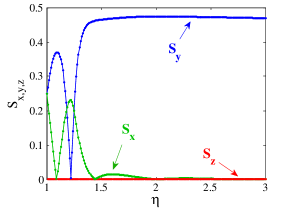
Figure 2: The quantities $S_{x,y,z}$, defined in Eq. 20 vs. the aspect ratio $\eta=L_{x}/L_{y}$ of a box with fixed area $\Omega=75/k_{0}^{2}$. When $L_{x}/L_{y}=1$, $S_{x}=S_{y}$; as $L_{x}/L_{y}$ increases, $S_{y}$ becomes close to $1$ and $S_{x}\rightarrow 0$.

The magnetic degrees of freedom in the anisotropic Wigner crystal can therefore be thought of as Ising-like spins, which are polarized in the $\pm\hat{y}$ directions. These spins are coupled by exchange processes, which generate N-body interactionsRoger (1984); Voelker and Chakravarty (2001); Bernu et al. (2001). In addition, because of the spin-orbit coupling, Van der Waals-like interactions generate spin-spin termsGangadharaiah et al. (2008), which are not exponentially suppressed in the Wigner crystal phase. A detailed estimate of these interactions is complicated, and we defer their analysis for later work.

V Smectic state

The anisotropic Wigner crystal variational wavefunction described above assumes that translational symmetry is broken. However, long-range quantum fluctuations can restore translational symmetry, either partially or fully, resulting in either a smectic state (which breaks translational symmetry in only one direction), a nematic state which breaks rotational symmetry but is translationally invariant, or an isotropic liquid. Since the ground state energy is mostly sensitive to short-range correlations, the crystal and the various liquid states can have close energies. Below, we demonstrate that one can write an explicit wavefunction describing a smectic state with the same parametric dependence of the ground state energy on density as that of the anisotropic WC. In the next section, a ferromagnetic nematic variational wavefunction will be described.

Let us consider, for simplicity, the case of short-range (contact) interactions. To construct a wavefunction for the smectic, we consider a trial Hamiltonian in which the electrons are confined to move along an array of strips of width $L_{y}$ with infinitely hard walls separating different strips. The problem is then reduced to finding the electronic ground state of a strip with a linear density of $nL_{y}$. The single-particle dispersion in the strip is derived in Appendix A (Eq. 37). The dispersion of the each transverse sub-band has two degenerate “valleys” at $\pm\left(k_{0}+\delta k_{x}^{\star}\right)$, where $\delta k_{x}^{\star}\sim 1/\left(k_{0}L_{y}^{2}\right)$. We will assume that only the lowest sub-band of the strip is occupied. (For a fixed $L_{y}$, this is valid for a sufficiently small densitycom (c).) Moreover, we may ignore the “valley” degeneracy since every electron can be assumed to be in one of the two valleys, and exchange processes between the valleys are suppressed. We thus obtain an effective one-dimensional Hamiltonian for the motion along a strip:

$$H=\sum_{i}\left(\Delta-\frac{\partial_{x}^{2}}{2m^{\star}}\right)+\frac{1}{2}\sum_{i,j}V\left(x_{i}-x_{j}\right),$$ (21)

where, from Eq.(37), $\Delta=A_{1}^{2}/8mk_{0}L_{y}^{4}$ and $m^{\star}\propto m$ ($A_{1}$ is a dimensionless constant). In the $n\rightarrow 0$ limit, the interaction becomes strong compared with the Fermi energy, and the electrons behave as effectively hard core particles (independently of their valley index). The system can be mapped onto a non-interacting spinless fermion problem. The ground state energy per particle is thus

$$\varepsilon\left(L_{y}\right)=\frac{A_{1}}{8mk_{0}^{2}L_{y}^{4}}+\frac{\left(\pi nL_{y}\right)^{2}}{6m^{*}}.$$ (22)

Minimizing this expression with respect to $L_{y}$, we obtain the ground state energy per particle of the smectic state:

$$\varepsilon_{\mathrm{SM}}\sim\frac{k_{0}^{2}}{m}\left(\frac{n}{k_{0}}\right)^{\frac{4}{3}}.$$ (23)

The scaling of the energy of the smectic state with $n$ is thus the same as that of the anisotropic Wigner crystal, Eq.(11)com (c). The numerical prefactor, which cannot be determined reliably from such simple considerations, is therefore important in determining which of these two states is favored in the $n\rightarrow 0$ limit.

In the case of extended interactions which decay with an exponent $\alpha$, one can use the same variational wavefunction for the smectic, in which the expectation value of the potential energy is finite, and then minimize the total energy over $L_{y}$. The calculation proceeds in essentially the same way as in Sec. III.3, and we will not repeat the details here. The result is that the parametric dependence of the smectic variational energy on $n$ is the same as that of the Wigner crystal, Eq.(18), for any $\alpha$.

VI Ferromagnetic nematic state

Finally, we consider a complete melting of the anisotropic Wigner crystal phase, preserving its preferred orientation. This results in a nematic state. Similarly to the situation in the Wigner crystal and the smectic states, we expect that in the low-density limit, only states in the vicinity of two opposite points $\pm\vec{k}_{0}$ on the ring of minimal dispersion will be occupied. For simplicity, we will assume the occupation is limited to the vicinity of only one point on the ring, $\vec{k}_{0}$, which makes the nematic state also ferromagnetic (with an in-plane magnetization perpendicular to $\vec{k}_{0}$). Such a state is particularly easy to describe within a Hartree-Fock approximation. We emphasize, however, that a paramagnetic nematic state is also possible, although it is not easily captured by a simple variational wavefunction.

The Hartree-Fock analysis of the ferromagnetic nematic state is straightforward, and is described in Appendix B. At a sufficiently low density, a spontaneous in-plane magnetization develops, and the Fermi surface becomes asymmetric. At asymptotically low densities, the Fermi surface becomes an ellipse centered around one of the points on the minimal dispersion ring in momentum space. The total variational ground state energy per particle in this limit scales with density as (see Eq. 49)

$$\varepsilon_{\mathrm{FM}}\sim\begin{cases}n^{2\left(1-\frac{1}{\alpha}\right)},&\alpha\leq 4\\ n^{\frac{3}{2}},&\alpha>4.\end{cases}$$ (24)

Comparing this to Eqs.(11),(18), and (23), we see that the ground state energy of the ferromagnetic state is parametrically smaller than that of either the anisotropic WC or the smectic states for $\alpha>3$, making it the best candidate for the ground state. For $2<\alpha\leq 3$, the scaling of the ground state energy with density of all three states has the same exponent. The energies differ only by the prefactor, which cannot be estimated reliably within the simple variational approach used here.

The ferromagnetic nematic state spontaneously breaks time reversal ($\mathcal{T}$) and rotational symmetry ($\mathcal{R_{\theta}}$) about the z axis, as well as the mirror symmetry, $\mathcal{M}_{y}$, for the plane parallel to the ferromagnetic moment. However, it preserves the product, $\mathcal{TR}_{\pi}$, of time-reversal and rotation by $\pi$ (hence the name, “nematic”) and reflection through the plane perpendicular to the moment, $\mathcal{M}_{x}$. The latter symmetry insures that there is no out-of-plane component of the magnetization, and no anomalous Hall effect. Note that, even though this state carries a finite crystal momentum, it does not carry a finite current density, as required by a theorem by F. BlochBlo ; Bohm (1949); com (d). There is, however, a large anisotropy in the in-plane Drude weight (effective mass). From our Hartree-Fock state (see Appendix B), we find that the anisotropy scales as $n^{2-\frac{4}{\alpha}}$ for $\alpha<4$, and as $n^{-1}$ for $\alpha\geq 4$, in the low-density limit.

The physics behind the formation of the in-plane ferromagnetic state is similar to the usual Stoner picture for ferromagnetism: the system gains exchange energy by polarizing, at the expense of kinetic energy. In a system with Rashba SOC at low density, the exchange energy gain exceeds the kinetic energy cost due to the high density of states. In the low-density limit, the Fermi surface becomes parametrically anisotropic. Qualitatively, the short-range correlations in this state are similar to those of the anisotropic Wigner crystal. This explains why these states are close in energy, at least for $\alpha\leq 3$. The long-range correlations, however, are very different: the ferromagnetic state is a fluid, whereas the Wigner crystal is an insulator.

VII Phase diagram

So far, we have argued that for sufficiently low density and for short-ranged interactions, the system breaks rotational invariance, going into either an anisotropic Wigner crystal, smectic, or a nematic state. We now discuss the global features of the phase diagram as a function of density and the interaction range. For concreteness, let us discuss a 2DEG with Rashba SOC with screened Coulomb interactions, where the screening is from a nearby metallic gate at a distance $\xi$ away. The effective electron-electron interaction is $V\left(r\right)\approx e^{2}/\kappa r$ for $r\ll\xi$, where $\kappa$ is the dielectric constant of the surrounding material, and $V\left(r\right)\sim e^{2}\xi^{2}/\kappa r^{3}$ for $r\gg\xi$.

The broken symmetry state forms at a density $n^{\star}$ at which various scales become comparable to each other. We define a density $n_{1}^{\star}$ at which the energy of the broken symmetry state per particle is comparable to that of the uniform Fermi liquid state (which is dominated by Coulomb energy):

$$\frac{e^{2}\xi n_{1}^{\star}}{\kappa}\sim\frac{1}{m}\left(m\frac{e^{2}\xi^{2}}{\kappa}\right)^{\frac{2}{3}}\left(n_{1}^{\star}\right)^{\frac{4}{3}},$$ (25)

where $e$ is the electron charge, and $\kappa$ is the dielectric constant of the host material. On the left hand side we have used that, for short range interactions, the potential energy of the uniform state scales linearly with density (assuming that $(n_{1}^{\star})^{-\frac{1}{2}}\gg\xi$), and on the right hand side we have used Eq.(18) for the energy of the broken symmetry state with $V_{0}\sim e^{2}\xi^{2}/\kappa$. Note that the energies of all the different candidate states are the same up to a numerical prefactor in the case $\alpha=3$; compare Eqs.(18) and (49). This gives $n_{1}^{\star}\sim\left(a_{0}\xi\right)$, where $a_{0}\equiv\kappa/me^{2}$ is the effective Bohr radius.

In addition, we define a density $n_{2}^{\star}$ at which the inter-electron distance is comparable to the screening length $\xi$, and a density $n_{3}^{\star}$ at which the Fermi wavevector is comparable to $k_{0}$. These characteristic densities are given by $n^{\star}<n_{2}^{\star}\equiv 1/\xi^{2}$ and $n^{\star}<n_{3}^{\star}\equiv k_{0}^{2}$. The strongly anisotropic states are favored at densities which satisfy $n<n^{\star}=\min[n_{1}^{\star},n_{2}^{\star},n_{3}^{\star}]$.

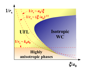
Figure 3: Sketch of the phase diagram of a 2DEG with Rashba SOC, as a function of $1/r_{s}\equiv a_{0}\left(\pi n\right)^{1/2}$ and the screening length $\xi$, where $a_{0}=\kappa/me^{2}$ is the Bohr radius. The three regions correspond to the uniform Fermi Liquid (UFL), the isotropic Wigner Crystal (WC), and a phase featuring a high degree of anisotropy, which can be either an anisotropic Wigner crystal, a smectic, or a nematic. The red dashed lines correspond to $r_{s}\sim\xi/a_{0}$, where the crossover between effectively short-range (screened) and long-range Coulomb interactions occurs; $1/r_{s}\sim k_{0}a_{0}$, where the SOC length scale becomes comparable to the inter-particle distance; and $1/r_{s}\sim(\xi/a_{0})^{-1/2}$, where the energies of the uniform Fermi liquid and the anisotropic phases become comparable, see Eq.(25).

We can now speculate about the structure of the zero temperature phase diagram of a 2DEG with Rashba SOC, sketched in Fig. 3, as a function of the dimensionless inter-electron spacing $r_{s}\equiv\left(\pi na_{0}^{2}\right)^{-1/2}$ and the screening length $\xi$. Let us consider large $\xi$, for which the Coulomb interactions are effectively unscreened. Then, a Wigner crystal with hexagonal symmetry forms when $r_{s}>r_{s,c}\approx 35$.Tanatar and Ceperley (1989) Imagine that we start deep in the Wigner crystal phase, with arbitrarily large $r_{s}$ and $\xi$. Upon decreasing $\xi$, while keeping $r_{s}$ fixed, eventually we reach $\xi\lesssim r_{s}a_{0}$, where the interactions are effectively short-ranged and the kinetic energy becomes important. At some point along this path, we expect a phase transition from the hexagonal Wigner crystal to one of the phases of lower rotational symmetry: either an anisotropic Wigner crystal, a smectic, or a nematic, which can also be ferromagnetic. Which of these phases is realized cannot be determined reliably on the basis of the present analysis.

At higher densities, such that $r_{s,c}<r_{s}<1/(k_{0}a_{0})$, the SOC can essentially be ignored. Then, upon decreasing $\xi$ from the Wigner crystal, we expect a transition to a Fermi liquid. The reentrant tip of the Wigner crystal phase originates from the same physical reasoning as that described in Ref Spivak and Kivelson, 2004.

As drawn, a sliver of UFL is shown between the isotropic WC and broken rotational symmetry phases. Such a region may or may not exist, depending on details of the numerical factors which are beyond the scope of the calculation here.

VIII Possible realizations

The physics described here could be relevant to electrons in two-dimensional heterostructures which lacks inversion symmetry, such as GaAlAs quantum wells. The magnitude of the Rashba spin-orbit coupling in these systems, however, is rather small. As discussed above, a necessary condition for realizing the phases with broken rotational symmetry is $r_{s}\gtrsim 1/k_{0}a_{0}$, or equivalently, $k_{F}\lesssim k_{0}$; in typical GaAlAs quantum wells, $k_{0}/k_{F}\sim 0.5$ or less, and the characteristic energy scale of the SOC, $E_{0}$ is at most of the order of a few degrees KelvinWin ; Nitta et al. (1997). More promising systems are surface states of heavy metal surface alloys. For instance, the boundary between Bi_xPb_1-x and Ag(111) supports a surface state with very strong Rashba SOC, with $k_{0}\approx 2\mathrm{nm}^{-1}$ and $E_{0}\approx 0.1\mathrm{eV}$.Ast et al. (2007a); Meier et al. (2009) Moreover, it was demonstrated that by varying $x$, the Fermi level of the surface state can be tuned to be lower than $E_{0}$.Ast et al. (2008) The Coulomb interactions on the surface are naturally screened by the metallic bulkcom (e). Detecting the broken rotational symmetry on the surface poses a challenge, because transport measurements would be dominated by the bulk. One possibility is to look for signatures of anisotropy in the finite-frequency response, e.g. in the optical conductivity, assuming that the anisotropic domains can be aligned (e.g., by application of an in-plane magnetic field). Scanning tunneling microscopy can be done on metallic surface alloysAst et al. (2007b), and used to detect anisotropy in the electronic structure. Finally, magnetic spectroscopy can be used to detect the ferromagnetic state, which has a large in-plane moment. Such measurements have recently been doneBert et al. (2011) on the conducting interface between LaAlO₃ and SrTiO₃, and indeed, large in-plane moments were found. Whether these are related to the mechanism described in this paper remains to be seen.

It has been proposedJung et al. (2011) that similar physics can arise lightly doped bilayer graphene with a perpendicular electric field, in which the single particle dispersion has a minimum on a ring in k-space, even without SOC. In bilayer graphene the single particle dispersion is valley and spin degenerate. The ground state is likely to have additional broken symmetries, lifting these degeneracies.

It is interesting to note that the considerations which lead to broken rotational symmetry at low densities are independent of the particle statistics, and are thus valid for two-component bosons with effective (isotropic) Rashba-like spin orbit interactions. Recently, various techniques were proposed to realize effective SOC in systems of trapped ultracold atomsStanescu et al. (2007); Campbell et al. (2011). The properties of such systems have been the subject of intense studyWu et al. (2011); Stanescu et al. (2008); Wang et al. (2010); Gopalakrishnan et al. (2011). Highly anisotropic phases may be accessible in such systems at sufficiently low densities. Indeed, it was foundGopalakrishnan et al. (2011) that the ground state breaks rotational symmetry at low densities, and that the ground state energy per particle scales as $n^{4/3}$ in the limit $n\rightarrow 0$, consistently with our results for the anisotropic WC and smectic phases with contact interactions.

IX Conclusions

In the presence of strong Rashba SOC, even short-range electron-electron interactions become important. As a result, the system is expected to form a broken symmetry state at low enough densities. In this work, we have shown that for sufficiently short-range interactions, states which break rotational symmetry are favored in the low-density limit. This is a consequence of the fact that the single-particle dispersion has a minimum on a ring of finite radius in $k$-space, rather than at a single point. This physics is not limited to the case of Rashba SOC; for instance, a similar situation arises in spin-imbalanced fermionic superfluids with no SOC, in which the majority-spin quasiparticles have a dispersion which is minimal near $k_{F}$,Yang and Sachdev (2006) or in bilayer graphene with a transverse electric fieldJung et al. (2011).

We believe that the variational wavefunctions and physical arguments proposed above capture the correct scaling of the ground state energy, which is found to be parametrically lower than other states (e.g. a uniform Fermi liquid or an isotropic Wigner crystal). However, this approach is too crude to answer some important, more detailed questions, such as discriminating between the different broken symmetry states considered here. For sufficiently short-range interactions (which fall off with an exponent larger than 3) a nematic ferromagnetic state has a parametrically lower energy than all the other states considered here, and is therefore the best candidate for the ground state. It is not clear, at this point, whether a non-magnetic nematic state is a competitor or not; such a state is harder to capture within a simple variational approach. More detailed calculations will be needed to determine the phase diagram for interactions which fall off with distance with a power of 3 or less. For instance, it may be interesting to treat this problem in an unrestricted Hartree-Fock approximation, which can be used to systematically improve the variational wavefunctions used in this work.

Edge states of surface alloys, such as the one discovered by Ast et al.Ast et al. (2007a), seem to be promising candidates to realize the anisotropic Wigner crystal phase, since they combine extremely strong Rashba SOC, a tunable Fermi energy, and screening due to the nearby metal. In a real system, however, disorder will inevitably play a major role. As a result, both the positional and orientational order are expected to be short-ranged. To detect the broken symmetry state on the surface, one can either resort to local probes (such as scanning tunneling spectroscopy), or find a way to align the orientational domains, e.g. by an in-plane magnetic field.

Appendix A Rashba particle in a box

The arguments presented in this paper rely on the solution of the quantum mechanical problem of a single particle with Rashba SOC in a rectangular box of size $L_{x}\times L_{y}$ with infinite potential walls. While the corresponding problem without spin-orbit coupling is trivial, with spin-orbit coupling the problem of boundary-condition matching with the multi-component wavefunction is highly non-trivial. The reason the problem with SOC is more difficult is that in this case, the Hamiltonian is no longer separable (i.e., it cannot be written as a sum of two commuting terms, one of which depends only on the $x$ coordinate and the other on $y$). A circular well can be solved exactlyTsitsishvili et al. (2004), thanks to its rotational invariance.

In this Appendix, we combine several approaches to deduce the asymptotic form of the ground state energy in the anisotropic, low–density limit, Eq. (9) of the main text. We first solve the problem exactly in the $L_{x}\rightarrow\infty$ limit (keeping $L_{y}$ fixed), and then provide an argument which yields the form of the leading corrections for finite $L_{x}$. Finally, we present numerical results supporting the analytical arguments.

A.1 Solution in the $L_{x}\rightarrow\infty$ limit

In the limit $L_{x}\rightarrow\infty$, the problem becomes translationally invariant in the $x$ direction. The eigenfunctions then take the form

$$\psi(x,y)=e^{ik_{x}x}\varphi(y),$$ (26)

where $\psi$, $\varphi$ are two–component spinors. We choose coordinates such that the walls are at $y=\pm L_{y}/2$. Then $\varphi(y)$ satisfies the boundary conditions

$$\varphi(\pm L_{y}/2)=\left(\begin{array}[]{c}0\\ 0\end{array}\right)\text{.}$$ (27)

Seeking a solution with energy $E=\varepsilon$, we get that the wavevector modulus $k=\sqrt{k_{x}^{2}+k_{y}^{2}}$ satisfies

$$\varepsilon=\frac{\left(k-k_{0}\right)^{2}}{2m}\text{.}$$ (28)

Fixing $k_{x}$, we find four allowed values of $k_{y}$, which we denote by $\pm k_{y,\pm}$:

$$k_{y,\pm}=\sqrt{\left(k_{0}\pm\sqrt{2m\varepsilon}\right)^{2}-k_{x}^{2}}\text{.}$$ (29)

Note that $k_{y,\pm}$ can be imaginary.

The wavefunction for the transverse motion takes the form

$$\varphi(y)=\sum_{\eta_{1},\eta_{2}=\pm}a_{\eta_{1}\eta_{2}}e^{i\eta_{1}k_{y,\eta_{2}}y}\left(\begin{array}[]{c}e^{-i\eta_{1}\theta_{\eta_{2}}/2}\\ ie^{i\eta_{1}\theta_{\eta_{2}}/2}\end{array}\right)\text{,}$$ (30)

where

$$e^{i\theta_{\eta_{1,2}}}=\frac{k_{x}+ik_{y,\eta_{1,2}}}{k}$$ (31)

and $a_{\eta_{1},\eta_{2}}$ ($\eta_{1},\eta_{2}=\pm$) are coefficients which are determined by the boundary conditions. We may reduce the number of coefficients by using symmetry. Under reflection, $y\rightarrow-y$ the spinor $\varphi(y)$ transforms as $\varphi(y)\rightarrow\sigma_{y}\varphi(-y)$. Requiring that the wavefunctions are either even or odd under reflection gives

$$a_{\eta_{1},\eta_{2}}=\pm a_{-\eta_{1},\eta_{2}}$$ (32)

Imposing the boundary condition, Eq. (27), on the wavefunction in Eq. (30), for the even sector gives the following (implicit) equation for $\varepsilon$:

$$\cos\left(\frac{k_{y,+}L_{y}}{2}-\frac{\theta_{+}}{2}\right)\cos\left(\frac{k_{y,-}L_{y}}{2}+\frac{\theta_{-}}{2}\right)-\cos\left(\frac{k_{y,+}L_{y}}{2}+\frac{\theta_{+}}{2}\right)\cos\left(\frac{k_{y,-}L_{y}}{2}-\frac{\theta_{-}}{2}\right)=0\text{,}$$ (33)

where $k_{y,\pm}$, $\theta_{\pm}$ are given by Eqs. (29) and (31). For the odd sector, we get an identical equation with $\cos$ replaced by $\sin$. Equation (33) determines the dispersion $\varepsilon(k_{x})$. The dispersion of the lowest subband, near $k_{x}=k_{0}$, is shown in Fig. 4, for widths $k_{0}L_{y}/2$ ranging from 10 to 20.

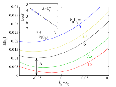
Figure 4: Dispersion of the lowest subband for infinite strips of varying width $L_{y}$. The inset shows the dispersion minimum $\Delta$ vs. $L_{y}$ on a log-log plot, showing good agreement with $\Delta\sim 1/L_{y}^{4}$.

The form of the low energy dispersion can be deduced from Eq. (33) as follows. To lowest order in $\varepsilon$ and $\delta k_{x}\equiv k_{x}-k_{0}$, this equation depends on $\varepsilon$, $\delta k_{x}$, and $L_{y}$ through the factors $k_{y,\pm}L_{y}:$

$$k_{y,\pm}L_{y} = \sqrt{\left(k_{0}\pm\sqrt{2m\varepsilon}\right)^{2}-\left(k_{0}+\delta k_{x}\right)^{2}}L_{y}$$ (34)

$$\approx \sqrt{\pm 2k_{0}\sqrt{2m\varepsilon}-2k_{0}\delta k_{x}}L_{y}.$$

Therefore Eq. (33) has the functional form

$$F\left(2k_{0}\sqrt{2m\varepsilon}L_{y}^{2},2k_{0}\delta k_{x}L_{y}^{2}\right)=0,$$ (35)

where $F$ is some function of two variables. Close to the band minimum, the dispersion has the following form:

$$2k_{0}\sqrt{2m\varepsilon}L_{y}^{2}=A_{1}+A_{2}\left[2k_{0}\delta k_{x}L_{y}^{2}-A_{3}\right]^{2},$$ (36)

where $A_{1,2,3}$ are dimensionless constants. Therefore

$$\varepsilon\left(\delta k_{x}\right) \approx \frac{1}{8mk_{0}^{2}}\left[\frac{A_{1}}{L_{y}^{2}}+A_{2}\left(2k_{0}\delta k_{x}-\frac{A_{3}}{L_{y}^{2}}\right)^{2}L_{y}^{2}\right]^{2}$$ (37)

$$\approx \frac{1}{8mk_{0}^{2}}\frac{A_{1}^{2}}{L_{y}^{4}}+\frac{A_{1}A_{2}}{m}\left(\delta k_{x}-\delta k_{x}^{\star}\right)^{2},$$

where $\delta k_{x}^{\star}=A_{3}/2k_{0}L_{y}^{2}$. We see the dispersion minimum $\Delta$ scales as $1/L_{y}^{4}$, while the effective mass in the $x$ direction is $L$ independent. We confirm the relation $\Delta\sim 1/L_{y}^{4}$ by solving Eq. (33) numerically, see inset of Fig. 4.

A.2 Extension to Finite $L_{x}$

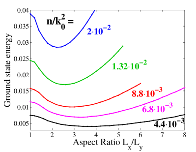
Figure 5: Numerical results for the ground state energy vs. aspect ratio $L_{x}/L_{y}$ of a particle with Rashba spin orbit coupling in a rectangular infinite potential well of size $L_{x}\times L_{y}$, for several values of the density $n$ (measured in units of $1/k_{0}^{2}$). We have set $2m=1$.

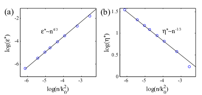
Figure 6: (a) Minimal ground state energy, $\varepsilon^{\star}$, and (b) optimal aspect ratio, $\eta^{\star}$, as a function of the density, on a log-log scale. The data is consistent with the analytical predictions: $\varepsilon^{\star}\sim n^{4/3}$ and $\eta^{\star}\sim n^{-1/3}$ at low densities.

Next, we consider that $L_{x}$ is finite, still assuming that $L_{x}\gg L_{y}$. In this case, the solution is complicated by multiple reflections from the boundaries. Nevertheless, we can deduce the form of the ground state energy as a function of $L_{x}$ and $L_{y}$ as follows. For large $L_{x}$, we assume that the solution is largely composed of traveling wave states near the bottom of the dispersion given by Eq. (37), which are reflected back and forth from the two edges. Consider a right-moving wave with momentum $k_{x}=k_{0}+\delta k_{x}$. This state can only be reflected to the state $k_{x}^{\prime}=k_{0}-\delta k_{x}+2\delta k_{x}^{\star}$, where $\delta k_{x}^{\star}$ is defined below Eq. (37). Note that time reversal symmetry prohibits scattering to the other left-moving solution with momentum $-k_{0}-\delta k_{x}$, since this state is the Kramer’s partner of the original incoming wave. The eigenstates of the system are determined by the requirement that the phase acquired over one period is a multiple of $2\pi$:

$$2\left(\delta k_{x}-\delta k_{x}^{\star}\right)L_{x}+\phi=2\pi j\text{,}$$ (38)

where $j$ is an integer, and $\phi=\phi_{1}+\phi_{2}$ is the sum of the two (unknown) phase shifts $\phi_{1}$, $\phi_{2}$ associated with reflections from the two ends. The total phase shift $\phi$ is a function $\delta k_{x}$, $L_{y}$ and $k_{0}$. However, in the limit $\delta k_{x}L_{y}\rightarrow 0$, $1/k_{0}L_{y}\rightarrow 0$, we assume that we can replace $\phi\left(\delta k_{x}L_{y},1/k_{0}L_{y}\right)$ by a constant $\phi\left(\delta k_{x}L_{y}\rightarrow 0,1/k_{0}L_{y}\rightarrow 0\right)\equiv\phi_{0}$. We then find that the ground state is given by $\delta k_{x}-\delta k_{x}^{\star}=(2\pi j_{\min}-\phi_{0})/2L_{x}$, where $j_{\min}$ is an integer chosen to minimize the energy below. Inserting this into Eq. (37), we finally get

$$\varepsilon\left(L_{x},L_{y}\right)\approx\frac{1}{8mk_{0}^{2}}\frac{A_{1}^{2}}{L_{y}^{4}}+\frac{A_{1}A_{2}\left(\pi j_{\min}-\phi_{0}/2\right)^{2}}{mL_{x}^{2}}\text{.}$$ (39)

Substituting $n=1/(L_{x}L_{y})$ and $\eta=L_{x}/L_{y}$, we obtain Eq. (11).

A.3 Numerical solution

In order to verify the assumptions that lead to Eq. (39), we have numerically calculated the ground state wavefunction of a Rashba particle in a box. This is done using a generalization of the “plane wave decomposition” technique described in Refs. Heller, 1984; Li et al., 1998. The solution is written as a superposition of eigenstates of the free Hamiltonian, which are plane waves with wavevectors satisfying Eq. (28) for some value of $\varepsilon$. The coefficients of the different plane waves are determined by requiring that both components of the wavefunction vanish on a set of points evenly distributed along the boundary (in this case, an $L_{x}\times L_{y}$ rectangle), and that the first component of the wavefunction spinor is equal to 1 at an arbitrary point in the interior. The sum of the squares of the wavefunction (the “tension”) at a different set of points on the boundary is then calculated. The eigenvalues $\varepsilon$ are identified as the minima of the tension. The eigenvalues can be determined with an accuracy of 1% or better. We have tested the technique by calculating the eigenenergies of a Rashba particle in a circular well, and found excellent agreement with the exact resultsTsitsishvili et al. (2004).

Fig. 5 shows the ground state energy vs. the aspect ratio $\eta=L_{x}/L_{y}$ for a few values of the density $1/n=L_{x}L_{y}$. The ground state energy is minimal for $\eta\neq 1$. We found this behavior for $n\lesssim 0.08k_{0}^{2}$; for higher densities (smaller box area), the minimum energy occurs at $\eta=1$. In Fig. 6 we show the minimal ground state energy $\varepsilon^{\star}$ and the corresponding aspect ratio $\eta^{\star}$ for densities ranging from $n/k_{0}^{2}=8\times 10^{-2}$ to $4\times 10^{-3}$. For low densities, the optimal ground state energy and aspect ratio follow $\varepsilon^{\star}\sim n^{4/3}$ and $\eta^{\star}\sim n^{-1/3}$, in agreement with Eqs. (10),(11), and (39).

Appendix B Hartree-Fock description of the ferromagnetic nematic

Within the Hartree-Fock approximation, we replace the full Hamiltonian $H$, Eq.(1), by the following mean-field Hamiltonian $\mathcal{H}$:

$$\mathcal{H}=\sum_{j}\left(\frac{1}{2m}\left[-\nabla_{j}^{2}-\frac{2k_{0}}{i}(\nabla_{j}\times{\hat{z}})\cdot\vec{\sigma}_{j}\right]-\mu-\frac{1}{2}\vec{h}\cdot\vec{\sigma_{j}}\right),$$ (40)

where $\vec{h}$ is a spontaneous Zeeman field, to be determined self-consistently, and $\mu$ is the chemical potential. We proceed by minimizing the expectation value of the full Hamiltonian within the ground state of the mean-field Hamiltonian, Eq.(40).

Let us focus on the case of an in-plane Zeeman field $\vec{h}$. (We will later argue that an out-of-plane $\vec{h}$ is not energetically favorable.) Without loss of generality, we assume that $\vec{h}=h\mathbf{\hat{x}}$. Then, the lower-branch single particle dispersion obtained by diagonalizing Eq.(40) is

$$\varepsilon_{k}=\frac{k^{2}}{2m}-\mu-\frac{k_{0}}{m}\sqrt{k_{x}^{2}+\left(k_{y}+\frac{mh}{2k_{0}}\right)^{2}}.$$ (41)

The minimum of the dispersion is obtained for $\vec{k}=k_{0}\mathbf{\hat{y}}$. In the low-density limit, only states close to the minimum are occupied. We therefore expand the dispersion around the minimum, using polar coordinates, $k_{x}=k\sin\theta$ and $k_{y}=k\cos\theta$ where $k=k_{0}+\delta k$, to leading order in $\delta k$ and $\theta$. This gives

$$\varepsilon_{k}\approx-\frac{k_{0}^{2}}{2m}-\frac{1}{2}h^{x}-\mu+\frac{\delta k^{2}}{2m}+\frac{1}{4}\frac{k_{0}^{2}h}{(k_{0}^{2}+\frac{m}{2}h)}\theta^{2}.$$ (42)

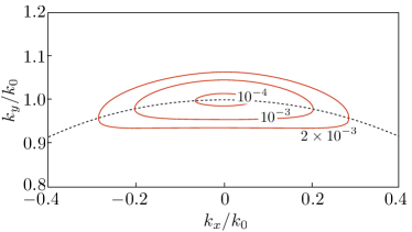
Figure 7: Constant energy contours of the dispersion of the mean-field Hamiltonian, Eq. 41, around the minimum at $\vec{k}=k_{0}\mathbf{\hat{y}}$. Numerical labels indicate energy values above the minimum, measured in units of $k_{0}^{2}/(2m)$. The dashed line indicates the circle $k_{x}^{2}+k_{y}^{2}=k_{0}^{2}$.

The Fermi surface is thus approximately an ellipse centered around $k_{0}\mathbf{\hat{y}}$ (see Fig.7). Denoting the Fermi energy measured relative to the dispersion minimum $\varepsilon_{0}=\frac{k_{0}^{2}}{2m}+\frac{1}{2}h^{x}+\mu$ as $\varepsilon_{F}$, we get that the density and Fermi energy are related by

$$n=\frac{m}{2\pi}\sqrt{1+\frac{2k_{0}^{2}}{mh}}\varepsilon_{F}.$$ (43)

The expectation value of the kinetic energy per particle in the ground state of $\mathcal{H}$ (measured relative to the band minimum, $\varepsilon_{0}$) is

$$K =\langle\mathcal{H}+\frac{1}{2}\vec{h}\cdot\vec{\sigma_{j}}\rangle+\frac{k_{0}^{2}}{2m}+\mu\approx\left\langle\frac{\delta k^{2}}{2m}\right\rangle$$

$$\approx\frac{\pi n}{2}\sqrt{\frac{h}{2mk_{0}^{2}}},$$ (44)

where we kept only the leading order term in $\frac{mh}{k_{0}^{2}}$. Next, we calculate the potential energy. Assuming that $V\left(r\right)\sim r^{-\alpha}$ at long distances, its Fourier transform has the following form for small momentum transfer:

$$\tilde{V}\left(q\right)\approx V_{0}\left(\beta_{0}-\beta_{1}q^{\alpha-2}\right)$$ (45)

for $2<\alpha\leq 4$, where we have neglected higher order terms in $q$. Here $\beta_{0}$ and $\beta_{1}$ are constants, and $V_{0}$ is defined in Eq.(2). For $\alpha>4$, the leading order term goes as $q^{2}$ (as can be seen, e.g., from the fact that for $\alpha>4$ the second moment of the potential exists). We now compute the potential energy

$$U =\frac{1}{2}\sum_{i,j}\left\langle V\left(\vec{r}_{i}-\vec{r}_{j}\right)\right\rangle$$

$$=\sum_{k,k^{\prime},q,\sigma,\sigma^{\prime}}\frac{\tilde{V}\left(q\right)}{\Omega^{3}}\left\langle c_{k+q,\sigma}^{\dagger}c_{k,\sigma}c_{k^{\prime}-q,\sigma^{\prime}}^{\dagger}c_{k^{\prime},\sigma^{\prime}}\right\rangle,$$ (46)

where $\Omega$ is the volume of the system, and we have introduced $c_{k,\sigma}$, the annihilation operator of an electron with momentum $k$ and spin $\sigma$. The calculation can be simplified significantly in the limit of small $mh/k_{0}^{2}$, in which the Fermi surface becomes parametrically eccentric. In that limit, only the dependence of $\tilde{V}_{q}$ on the momentum parallel to the major (long) axis of the Fermi surface is important. The result can be written as $U=U_{\uparrow\uparrow}+U_{\uparrow\downarrow}$, where $U_{\uparrow\uparrow}$ and $U_{\uparrow\downarrow}$ are the interaction energies between same spins and opposite spins, respectively, given (to leading order in $mh/k_{0}^{2}$) by

$$U_{\uparrow\uparrow} =A\left(\beta_{1}V_{0}\right)n\left[\left(\frac{k_{0}^{2}}{mh}\right)^{\frac{1}{4}}\sqrt{n}\right]^{\alpha-2},$$

$$U_{\uparrow\downarrow} =B\frac{\left(\beta_{0}V_{0}\right)n^{2}}{k_{0}^{2}}\sqrt{\frac{k_{0}^{2}}{mh}}.$$ (47)

Here, $A$ and $B$ are dimensionless constants. We can now minimize the total energy per particle, $\varepsilon=K+U_{\uparrow\uparrow}+U_{\uparrow\downarrow}$, with respect to the variational parameter $h$. In the $n\rightarrow 0$ limit, we find that $h^{\star}$, the optimal Zeeman field, is

$$h^{\star}\sim\begin{cases}\frac{k_{0}^{2}}{m}\left(m\beta_{1}V_{0}\right)^{\frac{4}{\alpha}}n^{2-\frac{4}{\alpha}},&\alpha<4\\ \beta_{0}V_{0}n,&\alpha>4.\end{cases}$$ (48)

Inserting $h^{\star}$ back into the expression for the total energy, we get that the ground state energy is

$$\varepsilon^{\star}\sim\begin{cases}\frac{1}{m}\left(mV_{0}\right)^{\frac{2}{\alpha}}n^{2\left(1-\frac{1}{\alpha}\right)},&\alpha<4\\ \frac{k_{0}^{2}}{m}\sqrt{m\beta_{0}V_{0}}\left(\frac{n}{k_{0}^{2}}\right)^{\frac{3}{2}}.&\alpha>4.\end{cases}$$ (49)

Finally, we argue that an out-of-plane Zeeman field, $h_{z}\neq 0$, is not energetically favorable. First, note that for an in-plane field, in the low-density limit ($n\rightarrow 0$) the kinetic energy per particle is unaffected because the Zeeman field becomes parallel to the spin-orbit field for all occupied states, allowing each particle to gain the Zeeman energy without changing its wavefunction. In contrast, in order for an electron to align its spin with an out-of-plane Zeeman field, its wavefunction must include hybridization with the excited band (with energy $\sim k_{0}^{2}/m$ above the lower band). In the hybrized state, the upper band is occupied with a probability $\sim(mh_{z}/2k_{0}^{2})^{2}$, leading to a kinetic energy cost $(k_{0}^{2}/2m)\times(mh_{z}/2k_{0}^{2})^{2}$. For contact interactions, the potential energy per particle is given by $E_{p}=\frac{1}{4}(U_{0}/n)(n^{2}-m_{z}^{2})$, where $m_{z}\approx nh_{z}/(k_{0}/m^{2})$ (here we use that for small $h_{z}$, the spin of each electron obtains a $z$-component given by the ratio of $h_{z}$ to the spin-orbit field). Therefore the potential energy gain from $z$-polarization is approximately $\frac{1}{4}U_{0}n(mh_{z}/k_{0}^{2})^{2}$. Compared with the kinetic energy cost, we see that the potential energy gain includes an extra factor of $n$, indicating that the cost of polarizing in the $z$-direction overwhelms the benefits in the low-density limit.

References

- Wigner (1934) E. Wigner, Physical Review 46, 1002 (1934).
- Tanatar and Ceperley (1989) B. Tanatar and D. Ceperley, Phys. Rev. B 39, 5005 (1989).
- Drummond and Needs (2009) N. Drummond and R. Needs, Phys. Rev. Lett. 102, 126402 (2009).
- Yoon et al. (1999) J. Yoon, C. Li, D. Shahar, D. Tsui, and M. Shayegan, Phys. Rev. Lett. 82, 1744 (1999).
- (5) E. I. Rashba, Fiz. Tverd. Tela (Leningrad) 2, 1224 (1960) [Sov. Phys. Solid State 2, 1109 (1960)].
- com (a) Note that this expression is not valid near , and therefore it does not have an symmetry. For , of course, a similar expression holds with .
- com (b) This can be seen, e.g., from the exact solution of a Rashba particle in a circular boxTsitsishvili et al. (2004).
- Roger (1984) M. Roger, Phys. Rev. B 30, 6432 (1984).
- Voelker and Chakravarty (2001) K. Voelker and S. Chakravarty, Phys. Rev. B 64, 235125 (2001).
- Bernu et al. (2001) B. Bernu, L. Cândido, and D. Ceperley, Phys. Rev. Lett. 86, 870 (2001).
- Gangadharaiah et al. (2008) S. Gangadharaiah, J. Sun, and O. Starykh, Phys. Rev. Lett. 100, 156402 (2008).
- com (c) For the optimal strip width, , the Fermi energy is of the same order of the inter-subband splitting, so the assumption that only the lowest subband is occupied may not be justified. Nevertheless, one can construct a variational wavefunction with a ground state energy which scales as in Eq. 23 by choosing with a sufficeintly small prefactor such that only the lowest subband is occupied.
- (13) Appendix to L. Brillouin, J. de phys. et. rad. 4, 334 (1933).
- Bohm (1949) D. Bohm, Physical Review 75, 502 (1949).
- com (d) The fact that the current is zero can be seen, in the low density limit, from the fact that the Fermi surface is an ellipse enlosing the point at which the group velocity is zero. See Appendix B.
- Spivak and Kivelson (2004) B. Spivak and S. A. Kivelson, Phys. Rev. B 70, 155114 (2004).
- (17) “Spin-orbit coupling effects in two-dimensional electron and hole systems”, by R. Winkler, Springer-Verlag (Berlin), 2003.
- Nitta et al. (1997) J. Nitta, T. Akazaki, H. Takayanagi, and T. Enoki, Phys. Rev. Lett. 78, 1335 (1997).
- Ast et al. (2007a) C. Ast, J. Henk, A. Ernst, L. Moreschini, M. Falub, D. Pacilé, P. Bruno, K. Kern, and M. Grioni, Phys. Rev. Lett. 98, 186807 (2007a).
- Meier et al. (2009) F. Meier, V. Petrov, S. Guerrero, C. Mudry, L. Patthey, J. Osterwalder, and J. Dil, Phys. Rev. B 79, 241408(R) (2009).
- Ast et al. (2008) C. Ast, D. Pacilé, L. Moreschini, M. Falub, M. Papagno, K. Kern, M. Grioni, J. Henk, A. Ernst, S. Ostanin, et al., Phys. Rev. B 77, 081407(R) (2008).
- com (e) In the case of a metallic surface alloy, we are assuming that the effect of the bulk electrons is mostly to screen the Coulomb interaction on the surface.
- Ast et al. (2007b) C. Ast, G. Wittich, P. Wahl, R. Vogelgesang, D. Pacilé, M. Falub, L. Moreschini, M. Papagno, M. Grioni, and K. Kern, Phys. Rev. B 75, 201401(R) (2007b).
- Bert et al. (2011) J. a. Bert, B. Kalisky, C. Bell, M. Kim, Y. Hikita, H. Y. Hwang, and K. a. Moler, Nature Physics 7, 767 (2011).
- Jung et al. (2011) J. Jung, M. Polini, and A. MacDonald, Arxiv preprint arXiv:1111.1765 (2011), eprint 1111.1765.
- Stanescu et al. (2007) T. Stanescu, C. Zhang, and V. Galitski, Phys. Rev. Lett. 99, 110403 (2007).
- Campbell et al. (2011) D. L. Campbell, G. Juzeliūnas, and I. B. Spielman, arXiv:1102.3945 (preprint) (2011).
- Wu et al. (2011) C.-J. Wu, I. Mondragon-Shem, and X.-F. Zhou, Chinese Physics Letters 28, 097102 (2011), eprint arXiv:0809.3532v5.
- Stanescu et al. (2008) T. Stanescu, B. Anderson, and V. Galitski, Phys. Rev. A 78, 023616 (2008).
- Wang et al. (2010) C. Wang, C. Gao, C.-M. Jian, and H. Zhai, Phys. Rev. Lett. 105, 160403 (2010).
- Gopalakrishnan et al. (2011) S. Gopalakrishnan, A. Lamacraft, and P. Goldbart, Physical Review A 84, 061604(R) (2011).
- Yang and Sachdev (2006) K. Yang and S. Sachdev, Phys. Rev. Lett. 96, 187001 (2006).
- Tsitsishvili et al. (2004) E. Tsitsishvili, G. Lozano, and A. Gogolin, Phys. Rev. B 70, 115316 (2004).
- Heller (1984) E. Heller, Phys. Rev. Lett. 53, 1515 (1984).
- Li et al. (1998) B. Li, M. Robnik, and B. Hu, Physical Review E 57, 4095 (1998).