Automatic asymptotics for coefficients of smooth, bivariate rational functions

Timothy DeVries

Joris van der Hoeven^,

Robin Pemantle^,

We consider a bivariate rational generating function

$$F(x,y)=\frac{P(x,y)}{Q(x,y)}=\sum_{r,s\geq 0}a_{rs}x^{r}y^{s}$$

under the assumption that the complex algebraic curve ${\mathcal{V}}$ on which $Q$ vanishes is smooth. Formulae for the asymptotics of the coefficients $\{a_{rs}\}$ are derived in [PW02]. These formulae are in terms of algebraic and topological invariants of ${\mathcal{V}}$, but up to now these invariants could be computed only under a minimality hypothesis, namely that the dominant saddle must lie on the boundary of the domain of convergence. In the present paper, we give an effective method for computing the topological invariants, and hence the asymptotics of $\{a_{rs}\}$, without the minimality assumption. This leads to a theoretically rigorous algorithm, whose implementation is in progress at http://www.mathemagix.org

Subject class: 05A15

Keywords: Rational function, generating function, Morse theory, Cauchy integral, Fourier-Laplace integral

1 Introduction

Consider a power series $F({\bf z})=\sum_{\bf r}a_{\bf r}{\bf z}^{\bf r}$, where ${\bf r}$ varies over integer vectors in the orthant $({\mathbb{Z}}^{+})^{d}$ and ${\bf z}^{\bf r}$ denotes the monomial $z_{1}^{r_{1}}\cdots z_{d}^{r_{d}}$. We say that $F$ is the (ordinary) generating function for the array $\{a_{\bf r}\}$. In analytic combinatorics, our aim is to derive estimates for $a_{\bf r}$, given a simple description of $F$ as an analytic function. An apparatus for doing this for various classes of function is developed in a series of papers [PW02, PW04, BP08, Pem10]; see also the survey [PW08]. Most known results on multivariate asymptotics concern either rational functions or quasi-powers. In the case of rational functions $F({\bf z})=P({\bf z})/Q({\bf z})$, the analysis centers on geometric properties of the pole variety ${\mathcal{V}}:=\{{\bf z}:Q({\bf z})=0\}$.

When ${\mathcal{V}}$ has singularities, tools are required such as iterated residues, resolution of singularities or generalized Fourier transforms, and analyses exist only for specific examples. When ${\mathcal{V}}$ is smooth, if certain degeneracies are avoided, asymptotic formulae for $a_{\bf r}$ may be given in terms of certain algebraic and topological invariants of ${\mathcal{V}}$. Denote normalized vectors by

$${\hat{\bf r}}:=\frac{{\bf r}}{|{\bf r}|}=\left(\frac{r_{1}}{\sum_{j=1}^{d}r_{j}},\ldots,\frac{r_{d}}{\sum_{j=1}^{d}r_{j}}\right):=(\hat{r}_{1},\ldots,\hat{r}_{d})\,.$$

Asymptotic formulae for $a_{\bf r}$ depend on the direction ${\hat{\bf r}}$ in which ${\bf r}$ is going to infinity. For example, Theorem 3.9 of [Pem10, Theorem 3.9] gives an asymptotic formula for $a_{\bf r}$ in terms of a sum over a set $\Xi$ of quantities that are easily computed via standard saddle point techniques. The set $\Xi=\Xi({\hat{\bf r}})$ is a subset of the set saddles of saddle points of the function $h:{\mathcal{V}}\to{\mathbb{R}}$ defined by

$$h({\bf z}):=h_{{\hat{\bf r}}}({\bf z}):=-\sum_{j=1}^{d}\hat{r}_{j}\log|z_{j}|\,.$$ (1.1)

The set saddles is readily computed but membership in the subset $\Xi$ is not easily determined, and in fact there is no known algorithm for doing so.

The main result in this paper is a characterization of $\Xi$ when $d=2$ and the complex algebraic curve ${\mathcal{V}}$ is smooth. This leads to a completely effective and rigorous algorithm for asymptotically computing $a_{\bf r}$. Precise statements of these results are somewhat technical, so we refer to the main text. The organization of the paper is as follows.

Section 2 reviews background results from elsewhere which reduce the computation of asymptotic formulae to identification of the set $\Xi$ and of some path segments through each $\sigma\in\Xi$. In particular, Section 2 begins with the integral representation of the general coefficient $a_{\bf r}$, Section 2.1 defines the residue of a meromorphic form, Section 2.2 reduces the integral for $a_{\bf r}$ to a lower-dimensional integral with some parameters yet to be specified, and Section 2.3 selects a chain of integration for this integral that results in an explicit asymptotic estimate in terms of saddles, $\Xi$ and the so-called critical height $c_{*}$ (Theorem 2.13).

The new material begins in Section 3. Beginning with the topology of ${\mathcal{V}}$ near the coordinate axes (Theorem 3.2), we give a topological characterization of the critical minimax height $c_{*}$ to which the cycle of integration can be lowered (Theorem 3.4) and of the set $\Xi$ of contributing saddles (Theorem 3.5). Section 4 demonstrates how these topological computations of $c_{*}$ and $\Xi$ can be made completely effective (Algorithm 4.8 and Theorem 4.9). Details of implementation are given, as well as a discussion of uniformity and boundary cases.

2 Background

In this section we review the framework for deriving estimates for $a_{\bf r}$, beginning with results for general $F$, then specializing to rational functions, and smooth pole variety ${\mathcal{V}}$. This section may be skipped by readers who want only to understand the effective computation and not the underlying analysis. Most of the material in this section is valid for any number of variables. When we need to assume a bivariate function, we will state this but will also change the notation to use $x$ and $y$ in place of $z_{1}$ and $z_{2}$ and $(r,s)$ in place of ${\bf r}$.

Computation of $a_{\bf r}$ via complex analytic methods begins with the multivariate Cauchy integral formula.

$$a_{\bf r}=\frac{1}{(2\pi i)^{d}}\,\int_{T}\frac{F({\bf z})}{z_{1}\cdot\ldots\cdot z_{d}}{\bf z}^{-{\bf r}}\,d{\bf z}\,.$$ (2.1)

Here the torus $T$ is any product of a circles in each coordinate sufficiently small so that the product of the corresponding disks lies completely with the domain of holomorphy ${\mathcal{D}}$ of $F$. This version of Cauchy’s formula can be found in most textbooks presenting complex analysis in a multivariable setting, and follows easily as an iterated form of the single variable formula; see, for example, [Sha92, page 19]. The integrand is may be written as ${\bf z}^{-{\bf r}}\omega$ where

$$\omega:=\omega_{F}:=\frac{F({\bf z})}{z_{1}\cdot\ldots\cdot z_{d}}\,d{\bf z}\,.$$ (2.2)

Let $({\mathbb{C}}^{*})^{d}:=({\mathbb{C}}\setminus 0)^{d}$ denote the set of complex $d$-vectors with all nonzero coordinates and denote ${\mathcal{V}}^{\prime}:={\mathcal{V}}\cap({\mathbb{C}}^{*})^{d}$. A key step in obtaining asymptotic estimates for $a_{\bf r}$ is to transform the Cauchy integral equation $(2\pi i)^{d}a_{\bf r}=\int_{T}{\bf z}^{-{\bf r}}\omega_{F}$ via an identity valid for any meromorphic form with a simple pole:

$$\int_{T}{\bf z}^{-{\bf r}}\omega=2\pi i\,\int_{\alpha}{\rm Res}\,({\bf z}^{-{\bf r}}\omega)$$ (2.3)

where ${\rm Res}\,(\cdot)$ is the residue operator defined in Section 2.1 and $\alpha$ is the intersection class defined in Section 2.2. Putting these together and specializing to $d=2$ leads to Lemma 2.4 below:

$$a_{\bf r}=\frac{1}{2\pi i}\,\int_{\alpha}x^{-r}y^{-s}\,{\rm Res}\,(\omega)\,.$$

2.1 The residue form

The residue form ${\rm Res}\,(\eta)$ is a holomorphic $(d-1)$-form on ${\mathcal{V}}^{\prime}$. The specification of this form will not be important for the subsequent analysis, but for completeness we include the following definition. If $\eta=(P/Q)\,d{\bf z}$ is any meromorphic form on a domain $U$ with simple pole on a set ${\mathcal{V}}\subseteq U$, then we define

$${\rm Res}\,(\eta):=\iota^{*}\theta\,$$ (2.4)

where $\theta$ is any solution to

$$dQ\wedge\theta=P\,d{\bf z}\,.$$ (2.5)

Existence and uniqueness are well known, and a proof can be found in [DeV10, Proposition 2.6] among other places (see, e.g., [AY83]). One important property of the residue form is that if $g:{\mathcal{V}}\to{\mathbb{C}}$ is holomorphic then

$${\rm Res}\,(g\cdot\eta)=g\cdot{\rm Res}\,(\eta)\,.$$

In particular, ${\rm Res}\,({\bf z}^{-{\bf r}}\,\omega)={\bf z}^{-{\bf r}}{\rm Res}\,(\omega)$.

2.2 The intersection class

Because ${\rm Res}\,({\bf z}^{-{\bf r}}\,\omega)$ is holomorphic on ${\mathcal{V}}^{\prime}$, the integral over a $(d-1)$-cycle $B\subseteq{\mathcal{V}}^{\prime}$ depends only on the homology class of $B$ in $H_{d-1}({\mathcal{V}}^{\prime})$. The chain of integration $\alpha$ in (2.3) is really a homology class known as the intersection class of $T$ with ${\mathcal{V}}^{\prime}$. The construction of the intersection class is quite general and may be found in the literature. Conditions are given in [PW12, Appendix A] for the intersection class to be uniquely defined. When it is not, however, the integral over $\alpha$ must be the same for any choice of intersection class, $\alpha$, so we will not pursue it further here.

Because we will need an explicit construction of a cycle in this class, we will give a quick construction of $\alpha$ and derivation of (2.3). We begin with a form of the Cauchy-Leray residue theorem, which may be found in [DeV10, Theorem 2.8].

Lemma 2.1 (Cauchy-Leray Residue Theorem).

Let $\eta$ be a meromorphic $d$-form on domain $U\subseteq{\mathbb{C}}^{d}$ with pole variety ${\mathcal{V}}\subseteq U$ along which $\eta$ has only simple poles. Let $N$ be a $d$-chain in $U$, locally the product of a $(d-1)$-chain $C$ on ${\mathcal{V}}$ with a circle $\gamma$ in the normal slice to ${\mathcal{V}}$, oriented as the boundary of a disk oriented positively with respect to the complex structure of the normal slice. Then

$$\int_{N}\eta=2\pi i\int_{C}{\rm Res}\,(\eta)\,.$$

$\hfill\Box$

Corollary 2.2.

Let $F,P,Q$ and ${\mathcal{V}}$ be as above and let $\eta$ be meromorphic. Let ${\mathcal{M}}_{1}$ and ${\mathcal{M}}_{2}$ be compact $d$-manifolds in ${\mathbb{C}}^{d}$ and let $H$ be a smooth homotopy from ${\mathcal{M}}_{1}$ to ${\mathcal{M}}_{2}$ that intersects ${\mathcal{V}}$ transversely in a compact manifold ${\mathcal{C}}$. Then

$$\int_{{\mathcal{M}}_{1}}\eta-\int_{{\mathcal{M}}_{2}}\eta=2\pi i\,\int_{{\mathcal{C}}}{\rm Res}\,(\eta)\,.$$

$\hfill\Box$

Proof: Let $N$ be the boundary of a tubular neighborhood $W$ of ${\mathcal{C}}$ in ${\mathbb{C}}^{d}$. Then $\eta$ is holomorphic on $H\setminus W$. The boundary of $H\setminus W$ is ${\mathcal{M}}_{2}-{\mathcal{M}}_{1}+N$, and $d\eta$ vanishes on $H\setminus W$ because the differential of any holomorphic $d$-form vanishes on ${\mathbb{C}}^{d}$. Tubular neighborhoods of a smooth algebraic hypersurface always have a product structure (see, e.g., [PW12, Proposition A.4.1]). Therefore, Stokes’ Theorem and Lemma 2.1 together yield

$$\int_{{\mathcal{M}}_{1}}\eta=\int_{{\mathcal{M}}_{2}}\eta+\int_{N}\eta=\int_{{\mathcal{M}}_{2}}\eta+2\pi i\,\int_{{\mathcal{C}}}{\rm Res}\,(\eta)\,.$$

$\hfill\Box$

Remarks 2.3.

One sees that the orientation of ${\mathcal{C}}$ must be chosen so that the boundary of its product with a positively oriented disk in the normal slice is homologous to ${\mathcal{M}}_{1}-{\mathcal{M}}_{2}$. Also note that result is true when $H\setminus W$ is any cobordism: we used only that $\partial(H\setminus W)={\mathcal{M}}_{2}-{\mathcal{M}}_{1}+N$, not that $H$ was a homotopy.

Let $T_{\epsilon}$ be the torus $\{|z_{1}|=\cdots=|z_{d}|=\epsilon\}$ and let $T_{\epsilon,L}$ be the torus $\{|z_{1}|=\cdots=|z_{d-1}|=\epsilon\,,|z_{d}|=L\}$. Fix $\epsilon>0$ and suppose that for sufficiently large $L$, the torus $T_{\epsilon,L}$ does not intersect ${\mathcal{V}}$. We claim that for $r_{d}$ sufficiently large,

$$\int_{T_{\epsilon,L}}{\bf z}^{-{\bf r}}\,\omega=0\,.$$ (2.6)

Indeed,

$$|{\bf z}^{-{\bf r}}\omega| \leq \epsilon^{-\sum_{j=1}^{d-1}r_{j}}L^{-r_{d}}\sup_{{\bf z}\in T_{\epsilon,L}}|\omega({\bf z})|$$

$$\leq CL^{-r_{d}}L^{\beta}$$

where $\beta$ is the degree of the rational form $\omega$. The chain of integration has volume $O(L)$, from which we conclude that $\int_{T_{\epsilon,L}}{\bf z}^{-{\bf r}}\,\omega=O(L^{1+\beta-r_{d}})$. Once $r_{d}>1+\beta$, we therefore have $\int_{T_{\epsilon,L}}{\bf z}^{-{\bf r}}\,\omega=o(1)$ as $L\to\infty$. But $T_{\epsilon,L}$ avoids ${\mathcal{V}}$ for sufficiently large $L$, hence by Stokes’ Theorem, $\int_{T_{\epsilon},L}{\bf z}^{-{\bf r}}\,\omega$ is constant for sufficiently large $L$, hence zero, establishing (2.6).

The intersection class may now be constructed as follows. Let $H_{L}$ be the homotopy defined by

$$H_{L}({\bf z},t)=(z_{1},\ldots,z_{d-1},(1-t)z_{d}+t(L/\epsilon-1)z_{d})\,.$$

Suppose that $H_{L}[T_{\epsilon}]$ intersects ${\mathcal{V}}$ transversely. We let

$$\alpha=[{\mathcal{C}}]~{}~{}~{}\mbox{ where }~{}~{}~{}{\mathcal{C}}:=H_{L}[T_{\epsilon}]\cap{\mathcal{V}}\,.$$ (2.7)

This is independent of $L$ once $L$ is sufficiently large. We take the orientation of ${\mathcal{C}}$ as in the remark following Corollary 2.2.

Summing up the residue and intersection cycle constructions we have:

Lemma 2.4 (Residue representation of $a_{\bf r}$).

Suppose $d=2$. Then for sufficiently small $\epsilon>0$,

$$a_{\bf r}=\frac{1}{(2\pi i)^{d-1}}\;\int_{\alpha}x^{-r}y^{-s}\,{\rm Res}\,(\omega)$$ (2.8)

holds with ${\rm Res}\,$ defined as in (2.4) – (2.5) and the intersection class $\alpha$ defined in (2.7).

Proof: Let $S$ be the set of $x\in{\mathbb{C}}$ such that there is a sequence $(x_{n},y_{n})$ in ${\mathcal{V}}$ with $x_{n}\to x$ and $y_{n}\to\infty$. The set $S$ is finite and therefore $\min\{|x|:x\in S,x\neq 0\}$ is strictly positive. Taking $\epsilon$ less than this minimum guarantees that for sufficiently large $L$, the torus $T_{\epsilon,L}$ does not intersect ${\mathcal{V}}$. The set of $(x,y)\in{\mathcal{V}}$ where $\partial Q/\partial y$ vanishes is also finite. Again, taking $\epsilon$ less than the least nonzero modulus of such a point guarantees that the homotopy $H_{L}$ intersects ${\mathcal{V}}$ transversely. Having verified these two suppositions, the construction of $\alpha$ is completed. Now apply Corollary 2.2 with ${\mathcal{M}}_{1}=T_{\epsilon},{\mathcal{M}}_{2}=T_{\epsilon,L},N={\mathcal{C}}$ and $\eta={\bf z}^{-{\bf r}}\omega$, where $\epsilon$ is small enough so that $T_{\epsilon}\subseteq{\mathcal{D}}$. Using (2.6) to see that $\int_{{\mathcal{M}}_{2}}\eta=0$ and combining with Cauchy’s integral formula gives

$$(2\pi i)^{d}a_{\bf r}=\int_{T_{\epsilon}}{\bf z}^{-{\bf r}}\omega=2\pi i\,\int_{\alpha}{\rm Res}\,({\bf z}^{-{\bf r}}\omega)=2\pi i\,\int_{\alpha}{\bf z}^{-{\bf r}}\,{\rm Res}\,(\omega)\,.$$

$\hfill\Box$

Remark 2.5.

The only use thus far of the restriction to $d=2$ is in verifying that $H_{L}$ intersects ${\mathcal{V}}$ transversely and $T_{\epsilon,L}$ not at all. Transversality may be accomplished for any $d$ via a perturbation and it is not hard to handle a nonempty intersection of ${\mathcal{V}}$ with $T_{\epsilon,L}$, so no essential use has been made yet of the restriction to $d=2$.

2.3 Morse theory

Saddle point integration techniques require that we choose a chain of integration ${\mathcal{C}}^{\prime}$ in the class $\alpha$ to (roughly) minimize the modulus of the integrand ${\bf z}^{-{\bf r}}\omega$. It will suffice to minimize the factor of ${\bf z}^{-{\bf r}}$, the form $\omega$ being bounded on compact chains. The log modulus of ${\bf z}^{-{\bf r}}$ is $\sum_{j=1}^{d}r_{j}\log|z_{j}|$. Letting $n=|{\bf r}|=\sum_{j=1}^{d}r_{j}$, we have

$$\log\left|{\bf z}^{-{\bf r}}\right|=\sum_{j=1}^{d}r_{j}\log|z_{j}|=nh_{{\hat{\bf r}}}({\bf z})$$

which explains our definition of $h$ in (1.1). It will be helpful to consider the manifold ${\mathcal{V}}^{\prime}$ from a Morse theoretic viewpoint with height function $h$.

Definitions 2.6.

Let ${\mathcal{M}}$ be any manifold and let $h:{\mathcal{M}}\to{\mathbb{R}}$ be any smooth, proper function with isolated critical points (a critical point is where $\nabla h$ vanishes). Let ${\mathcal{V}}^{\geq c}$ denote the subset of ${\mathcal{V}}$ consisting of points ${\bf z}$ with $h({\bf z})\geq c$. Define ${\mathcal{V}}^{>c},{\mathcal{V}}^{\leq c},{\mathcal{V}}^{<c}$ and ${\mathcal{V}}^{=c}$ similarly. Define the set ${\mbox{\elevenss saddles}}={\mbox{\elevenss saddles}}({\mathcal{M}},h)$ to be the set of critical points for $h$. The set $h[{\mbox{\elevenss saddles}}]$ is called the set of critical values. For fixed $(r,s)$, the set saddles is a zero-dimensional variety, whose defining equations we call the critical point equations:

$$Q(x,y) = 0$$ (2.9)

$$s\,x\,Q_{x}-r\,y\,Q_{y} = 0\,.$$

Here and henceforth, we use subscript notation for partial derivatives.

When $h:{\mathcal{V}}^{\prime}\to{\mathbb{R}}$ is the height function $h_{{\hat{\bf r}}}$ above, by convention we extend $h$ to ${\mathcal{V}}$ taking $h(0,y)=h(x,0)=+\infty$, so that points of ${\mathcal{V}}\setminus{\mathcal{V}}^{\prime}$ are in every ${\mathcal{V}}^{\geq c}$.

Theorem 2.7.

Let $h:{\mathcal{M}}\to{\mathbb{R}}$ be a smooth, proper function with isolated critical points.

1. Suppose there are no critical values of $h$ in the interval $[a,b]$. Then the gradient flow induces a homotopy in ${\mathcal{M}}$ between ${\mathcal{M}}^{\leq b}$ and ${\mathcal{M}}^{\leq a}$, and also between ${\mathcal{M}}^{\geq b}$ and ${\mathcal{M}}^{\geq a}$. This homotopy carries ${\mathcal{M}}^{=b}=\partial{\mathcal{M}}^{\geq b}=\partial^{{\mathcal{M}}\leq b}$ to ${\mathcal{M}}^{=a}$.

2. Let $a<c<b$ such that $c$ is the unique critical value of $h$ in $[a,b]$. Let $\sigma_{1},\ldots,\sigma_{k}$ enumerate the critical points of $h$ at height $c$. Then $H_{*}({\mathcal{M}}^{\leq b},{\mathcal{M}}^{\leq a})$ decomposes naturally as the direct sum of $H_{*}({\mathcal{M}}_{\sigma_{j}}^{\leq b},{\mathcal{M}}_{\sigma_{j}}^{\leq a})$, where ${\mathcal{M}}_{\sigma_{j}}$ is the intersection of ${\mathcal{M}}$ with a sufficiently small neighborhood of $\sigma_{j}$.

3. Let ${\mathcal{C}}$ be a cycle in ${\mathcal{M}}$ and let $c_{*}$ be the infimum of $c$ such that ${\mathcal{C}}$ is homologous in ${\mathcal{M}}$ to a cycle in ${\mathcal{M}}^{\leq c}$. Then $c$ is either $-\infty$ or a critical value, and in the latter case, for sufficiently small $\epsilon>0$, the cycle ${\mathcal{C}}$ projects to a nonzero homology class in $H_{*}({\mathcal{M}},{\mathcal{M}}^{\leq c-\epsilon})$.

Proof: Part $(i)$ is the first Morse lemma, a proof of which may be found for example in [Mil63, Theorem 3.1] or [GM88]. A generic perturbation separates the critical values, one may then prove part $(ii)$ by a standard excision argument. Part $(iii)$ is proved in [Pem10, Lemma 8]. $\hfill\Box$

Remark 2.8.

Classical Morse theory combines the first Morse lemma (no topological change between critical values) with a description of the change at a critical value (an attachment map). The results we have quoted require only the first Morse lemma. For this it is not necessary to assume $h$ is a Morse function, but only that it is a smooth, proper map with isolated critical points.

Example 2.9 (bivariate harmonic case).

Suppose $d=2$. Let $\sigma$ be a critical point of $h$ on ${\mathcal{V}}$ at height $c$ and suppose that locally $h$ is the real part of an analytic function. Then there is an integer $k\geq 2$ and there are local coordinates $\psi:U\to{\mathcal{V}}$ on a neighborhood of the origin in ${\mathbb{C}}^{1}$ such that $\psi(0)=\sigma$ and

$$h(\psi(z))=c+\;{\rm Re\,}\{z^{k}\}\,.$$

Figure 1 illustrates this for $k=4$. The shaded regions are where $h>c$. On the right, the connected local components of $\{h>c\}$ are number counterclockwise from 1 to $k$ and the local components of $\{h<c\}$ are numbered correspondingly.

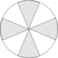
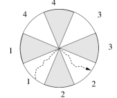
Figure 1: A saddle of order 4 and the path $\gamma_{1,2}$

The pair $\tilde{{\mathcal{M}}}:=({\mathcal{V}}^{\leq c+\epsilon}\cap\psi[U],{\mathcal{V}}^{\leq c+\epsilon}\cap\psi[U])$ is homotopy equivalent to a disk modulo $k$ boundary arcs. Let $\gamma_{j}$ denote an arc from the boundary to the center that remains in the $j^{th}$ local component of $\{h<c\}$. Then $H_{1}(\tilde{{\mathcal{M}}})$ is generated by the relative 1-cycles $\gamma_{i}-\gamma_{j}$. We have the relations $\sum_{i,j}b_{i,j}(\gamma_{i}-\gamma_{j})=0$ if and only

$$\sum_{j}b_{i,j}=\sum_{j}b_{j,i}$$

for every $i\leq k$. In particular, $\{\gamma_{i}-\gamma_{i+1}\;:\;1\leq i\leq k-1\}$ is a basis for $H_{1}(\tilde{{\mathcal{M}}})$.

We remark that our assumptions imply that $h$ has no local extrema on ${\mathcal{M}}$. Therefore, as $c$ decreases, the connected components of ${\mathcal{M}}^{\geq c}$ can merge but new components never arise.

This leads to a canonical form in dimension $d=2$ for classes in $H_{1}({\mathcal{V}}^{\prime})$, choosing a representing cycle so as to be in position for saddle point integration.

Proposition 2.10.

Let $h=h_{{\hat{\bf r}}}$. Let $\gamma$ be any cycle in $H_{1}({\mathcal{V}}^{\prime})$. Then either $\gamma$ is homologous to a cycle supported at arbitrarily small height or there is a critical value $c_{*}$ and a nonempty set $\xi\subset{\mbox{\elevenss saddles}}$ of critical points at height $c_{*}$ such that the following holds.

The cycle $\gamma$ is homologous in $H_{1}({\mathcal{V}}^{\prime})$ to a cycle ${\mathcal{C}}^{\prime}$ in ${\mathcal{V}}^{\leq c_{*}}$; the maximum of $h$ on ${\mathcal{V}}$ is achieved exactly on $\Xi$; in a neighborhood of each $\sigma\in\Xi$ of order $k=k(\sigma)\geq 2$, there is a subset ${\mbox{\elevenss paths}}(\sigma)$ of $\{1,\ldots,k(\sigma)-1\}$ such that the restriction of ${\mathcal{C}}^{\prime}$ to the neighborhood is equal to $\sum_{i\in T(\sigma)}\gamma_{i}-\gamma_{i+1}$.

As promised, integrals of the residue form ${\rm Res}\,(x^{-r}y^{-s}\omega_{F})$ are known. To summarize this, we let $F=P/Q$ be rational, with $\omega$ defined in (2.2) and ${\rm Res}\,(\omega)$ defined in Section 2.1. With $\gamma_{i}$ as in Figure 1, we then have the following explicit integration estimates. Note that the magnitude of $x^{-r}y^{-s}$ is $\exp[(r+s)c_{*}]$ when $(x,y)\in\Xi$, which makes the remainder term exponentially smaller than the summands.

Lemma 2.11 (saddle point integrals).

Let $\sigma=(x_{0},y_{0})\in{\mbox{\elevenss saddles}}$, satisfy the critical point
equations (2.9). Denote the order of vanishing of $h$ at $(x_{0},y_{0})$ by $k=k(x_{0},y_{0})$. Then
$(2\pi i)\int_{\gamma_{i}-\gamma_{i+1}}{\rm Res}\,(x^{-r}y^{-s}\omega)$ is given by the formula $\Phi(\sigma,i)$ where

$$\Phi(\sigma,i):=\frac{K(\sigma,i)}{\sqrt{2\pi(r+s)}}\,x_{0}^{-r}y_{0}^{-s}+O\left(\exp[(c_{*}-\epsilon)(r+s)]\right)$$ (2.10)

where $K(\sigma,i)$ is a constant term given by (2.11) when $d=2$ and more generally by an explicit formula which may be written in a number of ways, e.g. [PW02, Theorem 3.5] or [BBBP08, Theorem 3.3]. When $k=2$, the remainder term is uniform as $(x_{0},y_{0},r,s)$ varies with $(x_{0},y_{0})\in{\mbox{\elevenss saddles}}(r,s)$ and $(x_{0},y_{0})$ varying over a compact set on which $k$ is constant. When $k>2$, the estimate is uniform for fixed $(x_{0},y_{0})$ and $(r,s)\to\infty$ with $r=\lambda s+O(1)$, where $\lambda=xQ_{x}/(yQ_{y})$ evaluated at $(x_{0},y_{0})$. $\hfill\Box$

Remarks 2.12.

1. In fact a uniform estimate holds for $r=\lambda s+O(s^{1/2})$ although this is more complicated and involves Airy functions.

2. When $d=2$ the constant $K(\sigma,i)$ is given in [PW02, Theorem 3.1] as

   $$K(\sigma,i)=P(x,y)\sqrt{\frac{r+s}{s}\,\frac{-Q_{y}}{x\,\psi}}$$ (2.11)

   evaluated at $(x_{0},y_{0})$, where $\psi(x,y)$ is the expression in equation (4.4) below.

3. When $k>2$, the constant $K(\sigma,i)$ is the leading term in a series expansion for $\lambda$ near $\sigma$. The explicit formula involves partial derivatives of $P$ and $Q$ up to order $k$ and may be derived from, e.g., [PW02, Theorem 3.3].

Putting together Lemma 2.4 with Proposition 2.10 and Lemma 2.11 leads to the following asymptotic expression for $a_{\bf r}$, which has appeared several times before; for example, when $\sigma$ is a minimal point, this goes back to [PW02, Theorem 3.1]; for an alternative formulation see [BBBP08, Theorem 3.3].

Theorem 2.13 (smooth point asymptotics).

$$a_{rs}=\left(\frac{1}{2\pi i}\right)^{d-1}\sum_{\sigma\in\Xi}\;\;\;\sum_{i\in{\mbox{\elevenss paths}}(\sigma)}\Phi(\sigma,i)+O\left(\exp[(c_{*}-\epsilon)(r+s)]\right)\,.$$

$\hfill\Box$

This completes the summary of known results. We now turn to the main work which is to identify and compute the quantities $c_{*},\Xi$ and ${\mbox{\elevenss paths}}(\sigma)$ appearing in Theorem 2.13 and formula (2.10).

3 Identifying $c_{*}$ and $\Xi$

We begin by constructing the intersection class. We will take a homotopy which keeps the torus small in the $x$-coordinate. If ${\mathcal{V}}$ intersects the $y$-axis transversely at $(0,y)$, then the set ${\mathcal{V}}\cap\{|x|\leq\epsilon\}$ will have a component that is a topological disk nearly coinciding with a component of ${\mathcal{V}}^{\geq c}$ with $c=-\hat{r}\log\epsilon$. To see that something like this holds more generally, we recall some facts about Puiseux expansions. Consider the multivalued function $x\mapsto y(x)$ that solves $Q(x,y(x))=0$. When $x$ is in a sufficiently small punctured neighborhood of 0, there is a finite collection of convergent series of the form

$$y(x)=\sum_{j\geq j_{0}}c_{j}x^{j/k}$$ (3.1)

where $j_{0}\in{\mathbb{Z}}$, $k\in{\mathbb{Z}}^{+}$, and $c_{j_{0}}\neq 0$; such a series yields $k$ different values of $y$ for each $x$; together, the collection of series yields each solution to $Q(x,y)=0$ exactly once. We always assume that $k$ is chosen as small as possible. A proof of these facts may be found in [FS09, Theorem VII.7]. Our assumption that $Q(0,0)\neq 0$ implies $j_{0}\leq 0$ in every Puiseux series solution. Those with $j_{0}=0$ correspond to points at which ${\mathcal{V}}$ intersects the $x$-axis, the $y$-value being equal to the coefficient $c_{0}$. Under the assumption that ${\mathcal{V}}$ is smooth, for each such $y$-value there will be only one series. If $k=1$, the intersection with the $y$-axis is transverse but it is possible that $k\geq 2$ and ${\mathcal{V}}$ is smooth but with non-transverse intersection. Finally, series with $j_{0}<0$ correspond to components of ${\mathcal{V}}\cap\{|x|\leq\epsilon\}$ with $y$ going to infinity as $x$ goes to zero. We begin by showing that each series gives a single component and describing the embedding of the component. First, to clarify, we give an example in which all these possibilities occur.

Example 3.1.

Let $Q(x,y)=1-3y+2y^{2}-6xy^{4}+x^{3}y^{5}$. It is easy to check that ${\mathcal{V}}$ is smooth. The total number of solutions should be the $y$-degree of $Q$, namely 5. Setting $x=0$ we find two points $(0,1)$ and $(0,1/2)$ of ${\mathcal{V}}$ on the $y$-axis. These correspond to two series solutions with $j_{0}=0$ and $k=1$:

$$y(x) = 1+6x+72x^{2}+\cdots$$

$$y(x) = \frac{1}{2}-\frac{3}{8}x+\frac{45}{32}x^{2}+\cdots$$

There are also two series solutions with $j_{0}<0$, one with $k=1$ and one with $k=2$:

$$y(x) = \frac{1}{\sqrt{3}}x^{-1/2}-\frac{3}{4}+\frac{19\sqrt{3}}{32}x^{1/2}+\cdots$$

$$y(x) = 6x^{-2}-\frac{1}{18}x+\frac{1}{72}x^{3}\cdots\,.$$

The former of these yields two solutions. Although we do not need it here, we remark that these five solutions can be enumerated by counting $y$-displacement along the Northwest boundary of the Newton polygon: going up from $(0,0)$ to $(0,2)$ counts the first two solutions, going from $(0,2)$ to $(1,4)$ yields the two solutions $y\sim\pm 1/\sqrt{3x}$ and going from $(1,4)$ to $(3,5)$ yields the solution $y\sim 6x^{-2}$.

Let $X^{\geq c}$ (respectively $Y^{\geq c}$ denote the union of those components of ${\mathcal{V}}^{\geq c}$ containing arbitrarily small values of $x$ (respectively $y$). Say that the direction of a Puiseux series solution to $Q(x,y(x))=0$ is $-j_{0}/k$. The direction is always nonnegative because $j_{0}$ is nonpositive due to $Q(0,0)\neq 0$. Let

$${\mbox{\elevenss bad}}:=\{\beta>0\,:\,\beta\mbox{ is a direction of a series solution to }Q(x,y(x))=0\}$$

denote the set of positive directions.

Theorem 3.2 (${\mathcal{V}}^{\prime}$ near the axes).

Fix ${\hat{\bf r}}$ with $r/s\notin{\mbox{\elevenss bad}}$. Suppose that $h$ has isolated critical points. Then when $\epsilon>0$ is sufficiently small and $c$ is sufficiently large, the following hold.

1. The graph of each Puiseux expansion of $y(x)$ over the punctured disk $\{0<|x|<\epsilon\}$ is a component of ${\mathcal{V}}^{\prime}\cap\{|x|\leq\epsilon\}$.

2. Each such component is a topological disk and its boundary winds $k$ times around the $y$-axis.

3. The components of $X^{\geq c}$ are exactly the graphs over some neighborhood of 0 of those Puiseux series whose directions are less than $r/s$.

4. Components of ${\mathcal{V}}^{\prime}\cap\{|x|<\epsilon\}$ and $X^{\geq c}$ with the same Puiseux series are homotopic in ${\mathcal{V}}^{\prime}$.

Proof: Fix any Puiseux series solution $\sum_{j\geq j_{0}}c_{j}x^{j/k}$ on a punctured disk $U$ and define $g(x):=\sum c_{j}x^{j}$. From this we define the function

$$G:U \longrightarrow D$$

$$x \longmapsto(x^{k},g(x))\,.$$

We will show that $G$ is a diffeomorphism onto its image. For sufficiently small $\epsilon$ the images of the punctured $\epsilon$-disk under different Puiseux series are disjoint, which will finish the proof of $(i)$ and $(ii)$.

First we check that $G$ is one-to-one on a sufficiently small punctured disk. If not then we may find arbitrarily small $x_{1}$ and $x_{2}$ such that $x_{1}^{k}=x_{2}^{k}$ and $g(x_{1})=g(x_{2})$. This means that there is some $k^{th}$ root of unity $\xi$ and such that $g(x)=g(\xi x)$ for arbitrarily small $x$. For some $m$, the functions $x^{m}g(x)$ and $x^{m}g(\xi x)$ are holomorphic, and if they agree on a sequence converging to zero then they must define the same function on $U$. It follows that their Taylor expansions agree, and hence that the only nonzero coefficients are those indexed by a multiple of $k$. This contradicts the minimality of $k$ in the Puiseux series representation and we conclude that $g$ is one-to-one on a sufficiently small disk. For any smooth function $\phi$, the function $(x^{k},\phi(x))\mapsto x$ is diffeomorphism near any $x\neq 0$ because $x^{k}\mapsto x$ is locally smooth except at 0. This proves that $G$ is a diffeomorphism onto its image, establishing $(i)$ and $(ii)$. To continue, we need a lemma.

Lemma 3.3.

When $\epsilon$ is sufficiently small, for any $\theta$ the radial arcs

$$t\mapsto(te^{i\theta},y(te^{i\theta})),\;0\leq t\leq\epsilon$$

are monotone in height, that is,

$$h_{\theta}(t):=h(te^{i\theta},y(te^{i\theta}))$$

is monotone increasing or decreasing. Furthermore, as $t\downarrow 0$, $h_{\theta}(t)\to\pm\infty$ according to whether the direction $\beta=-j_{0}/k$ of the Puiseux series is less or greater than $r/s$.

Proof: Write

$$y(x)=cx^{-\beta}(1+\phi(x))$$

where the remainder $\phi$ satisfies $\phi(x)=o(1)$ and $x\phi^{\prime}(x)=o(1)$ as $x\to 0$. Plugging this into the function $H(x,y):=-\hat{r}\log x-\hat{s}\log y$ gives

$$\frac{d}{dx}H(x,y(x)) = \frac{\hat{s}\beta-\hat{r}}{x}-\frac{\phi^{\prime}(x)}{1+\phi(x)}$$ (3.2)

$$= \frac{1}{x}\left(\hat{s}\beta-\hat{r}-\frac{x\phi^{\prime}(x)}{1+\phi(x)}\right)$$

$$\sim \frac{\hat{s}\beta-\hat{r}}{x}$$

because we have assumed $\hat{s}\beta-\hat{r}\neq 0$. The function $h$ is the real part of $H$, which along with the chain rule yields

$$\frac{d}{dt}h_{\theta}(t)=\cos\theta\;{\rm Re\,}\frac{d}{dx}H(x,y(x))-\sin\theta\;{\rm Im\,}\frac{d}{dx}H(x,y(x))\,.$$

Plugging in (3.2) then gives

$$\frac{d\,h_{\theta}(t)}{dt}\sim\frac{\hat{s}\beta-\hat{r}}{|x|}$$

which finishes the proof of the lemma. $\hfill\Box$

Proof of Theorem 3.2, continued: Each component $B$ of $X^{\geq c}$ has, by definition, points with arbitrarily small values of $x$ which are therefore on the graph of one of the Puiseux series. Taking a sufficiently small neighborhood, the graphs of the series are disjoint, therefore the map from component to series is well defined. We need to see that the range of the map from components to series is exactly those with directions les than $r/s$. If $B$ has direction less than $r/s$ then $h\to\infty$ as $x\to 0$ on the corresponding component, whence the corresponding component of ${\mathcal{V}}^{\prime}\cap\{|x|<\epsilon\}$ maps to $B$. On the other hand, if the direction of $B$ is greater than $r/s$ then $h\to-\infty$ as $x\to 0$, from which it follows that $X^{\geq c}$ cannot contain points in $B$ with arbitrarily small $x$ values and hence such a component is not the graph of a Puiseux series about $x=0$. This proves $(iii)$.

Let $B$ be a component of $X^{\geq c}$ where $c$ is sufficiently large so that the projection onto $x$ is contained in a sufficiently small disk so that Lemma 3.3 applies. A radial homotopy in the $x$-coordinate (one that maps $x:=\rho e^{i\theta}$ to $f(\theta)x$ and maps $y(x)$ to $y(f(\theta)x)$) then shrinks $B$ to the same component with any specified greater value of $c$, or the corresponding component of ${\mathcal{V}}^{\prime}\cap\{|x|\leq\epsilon\}$ with as long as $\epsilon$ is at most the in-radius of the original $x$-neighborhood. This establishes $(iv)$ and also that either type of component remains in the same homotopy class as $c$ or $\epsilon$ is varied. $\hfill\Box$

Switching the roles of $x$ and $y$ in Theorem 3.2, it follows that for sufficiently large $c$, the set ${\mathcal{V}}^{\geq c}$ is the disjoint union of $X^{\geq c}$ and $Y^{\geq c}$. Define $c_{\rm xy}$ to the least value of $c$ for which this remains true, which is also that greatest value of $c$ such that ${\mathcal{V}}^{\geq c}$ has a component containing both a point $(0,y)$ and a point $(x,0)$. By the first Morse lemma, if $h$ is smooth and proper, the topology of ${\mathcal{V}}^{\geq c}$ cannot change between critical values of $h$. In particular $c_{\rm xy}$ must be a critical value $c_{j}$. The next two results complete the description of $c_{*}$ and $\Xi$.

Theorem 3.4 (characterization of $c_{*}$).

Assume that ${\mathcal{V}}$ is smooth and that $h=h_{{\hat{\bf r}}}$ is smooth and proper with isolated critical points. Then

1. For each $c\geq c_{\rm xy}$, the cycle $\partial X^{\geq c}$ is in the homology class $\alpha$ from Lemma 2.4.

2. $c_{*}=c_{\rm xy}$.

For each critical point $\sigma$ with $h(\sigma)=c_{*}$ let $k=k(\sigma)$ denote its order, let ${\mathcal{N}}$ denote a small neighborhood of $\sigma$ in ${\mathcal{V}}$. Label the components of ${\mathcal{N}}\cap\{h>c_{*}\}$ in counterclockwise order by $R_{1},\ldots,R_{k}$ as in Figure 1. Each such region $R$ will be called an $x$-region if $R\subseteq X^{>c}$ and a $y$-region if $R\subseteq Y^{>c}$. Because $c\geq c_{\rm xy}$, these are mutually exclusive.

Theorem 3.5 (characterization of $\Xi$ and paths).

1. $\sigma\in\Xi$ if and only if the regions $R_{1},\ldots,R_{k}$ include at least one $x$-region and at least one $y$-region.

2. Let $Y(j)=1$ if $R_{j}$ is a $y$-region and $Y(j)=0$ otherwise. Let ${\mathcal{C}}_{\sigma}$ denote the relative cycle in $H_{1}({\mathcal{N}}\cap{\mathcal{V}}^{c_{*}+\epsilon},{\mathcal{N}}\cap{\mathcal{V}}^{c_{*}-\epsilon})$ represented by

   $$\sum_{j=1}^{k}[Y(j)-Y(j+1)]\,\gamma_{j}$$

   Then ${\mathcal{C}}_{\sigma}$ represents the projection of $\alpha$ to this homology group, from which we easily recover ${\mbox{\elevenss paths}}(\sigma)$.

3. The cycle ${\mathcal{C}}_{*}:=\sum_{\sigma\in\Xi}{\mathcal{C}}_{\sigma}$ represents the projection of $\alpha$ to $H_{1}({\mathcal{V}}^{c_{*}+\epsilon},{\mathcal{V}}^{c_{*}-\epsilon})$.

$\hfill\Box$

Proofs: Let $c_{1}>\cdots>c_{\nu}=c_{xy}$ be the critical values of $h$ that are at least $c_{xy}$. Let ${\cal W}$ denote the set of $c\in{\mathbb{R}}$ for which $\partial X^{\geq c}\in\alpha$. To establish $(i)$ we will show:

1. If $c\in{\cal W}$ and $c_{i}>c>c_{i+1}$ then the entire closed interval $[c_{i+1},c_{i}]$ is a subset of ${\cal W}$;

2. If $c\in{\cal W}$ and $c>c_{1}$ then $[c_{1},\infty)\subseteq{\cal W}$;

3. If $c_{i}\in{\cal W}$ and $i<\nu$ then $c_{i}-\epsilon\in{\cal W}$ for all sufficiently small $\epsilon>0$;

4. The set ${\cal W}$ contains some $c>c_{1}$.

By part (i) of Theorem 2.7, the spaces $\{\partial X^{\geq t}\;:\;cI>t>c_{i+1}$ are all homotopic in ${\mathcal{V}}^{\prime}$, hence represent the same homology class in $H_{1}({\mathcal{V}}^{\prime})$. By continuity, this is true as well for $t=c_{i}$ and $t=c_{i+1}$, which proves (a). The proof of (b) is identical.

To prove (c), we first assume that there is a single critical point $\sigma$ with $h(\sigma)=c_{i}$. Let $k\geq 2$ be the order to which the derivatives of $h$ vanish at $\sigma$. Recall the neighborhood $U$ from Example 2.9 and the analytic parametrization $\psi:U\to{\mathcal{V}}$ with $h(\psi(z))=c_{i}+\;{\rm Re\,}\{z^{k}\}$. Locally, the image of $U$ is divided into $2k$ sectors with $h>c_{i}$ and $h<c_{i}$ in alternating sectors. Figure 2 shows ${\mathcal{V}}^{\geq c}$ (shaded) for three values of $c$ in the case $k=2$. A circle is drawn to indicate a region of parametrization for which $h=c_{i}+\;{\rm Re\,}\{z^{k}\}$. In the top diagram $c>c_{i}$, in the middle diagram $c=c_{i}$ and in the bottom, $c<c_{i}$. The arrows show the orientation of $\partial{\mathcal{V}}^{\geq c}$ inherited from the complex structure of ${\mathcal{V}}$. The pictures for $k>2$ are similar but with more alternations.

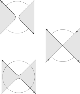
Figure 2: ${\mathcal{V}}^{\geq c}$ and its boundary for three values of $c$

Consider the first picture where $c>c_{i}$. Because $c>c_{xy}$, each of the $k$ shaded regions is in $X^{\geq c}$ or $Y^{\geq c}$ but not both. Let us term these regions “$x$-regions” or “$y$-regions” accordingly. Because $c_{i}>c_{xy}$, this persists in the limit as $c\downarrow c_{i}$, which means that either all $k$ regions are in $Y^{\geq c}$ or all $k$ regions are in $X^{\geq c}$. In the former case, $\partial X^{\geq c}$ does not contain $\sigma$ for $c$ in an interval around $c_{i}$ and the first Morse lemma shows that $\partial X^{\geq c_{i}+\epsilon}$ is homotopic to $\partial X^{\geq c_{i}-\epsilon}$. In the latter case we consider the cycle $\partial X^{\geq c_{i}+\epsilon}+\partial B$ where $B$ is the polygon showed in Figure 3. Because we added a boundary, this is homologous to $\partial X^{c_{i}+\epsilon}$. But also it is homotopic to $\partial X^{c_{i}+\epsilon}$: within the parametrized neighborhood, the lines may be shifted so as to coincide with $\partial X^{c_{i}+\epsilon}$, while outside this neighborhood the downward gradient flow provides a homotopy. In the case where there is more than one critical point at height $c_{i}$, we may add the boundary of a polygon separately near each critical $x$-point, that is, each point that is a limit as $\epsilon\downarrow 0$ of points in $X^{c_{i}+\epsilon}$.

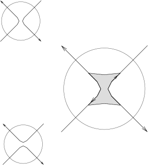
Figure 3: ${\mathcal{V}}^{\geq c_{i}+\epsilon}$ and ${\mathcal{V}}^{\geq c_{i}-\epsilon}$ differ locally by a boundary

Finally, we recall from Lemma 2.4 that a cycle ${\mathcal{C}}$ representing $\alpha$ is constructed as $H_{L}[T_{\epsilon}]\cap{\mathcal{V}}$. Here $\epsilon$ is sufficiently small and $L$ sufficiently large that this set is precisely $\{(x,y)\in{\mathcal{V}}:|x|=\epsilon\}$. By part $(iv)$ of Theorem 3.2, the union of these homotopic to $\partial X^{\geq c}$ for sufficiently large $c$. Checking that the orientation given by Remark 2.3 is the same as taking boundaries of regions oriented by the complex structure of ${\mathcal{V}}$, we conclude (d). Part $(i)$ of Theorem 3.4 is a direct consequence of (a) – (d).

Part $(i)$ implies that for any $c\geq c_{\rm xy}$, there is a cycle in the class $\alpha$ that is supported on ${\mathcal{V}}^{\geq c}$, which shows that $c_{*}\leq c_{\rm xy}$. To see that $c_{*}\geq c_{\rm xy}$, we suppose not and argue by contradiction. The construction in [Pem10, Lemma 3.8] shows that for each $c_{i}>c_{*}$, there is a cycle representing $\alpha$ supported on ${\mathcal{V}}^{\leq c_{i}+\epsilon}$ and any such cycle projects to zero in the relative group $({\mathcal{V}},{\mathcal{V}}^{c_{i}-\epsilon})$. For a contradiction, it suffices to check that $\partial X^{c_{*}+\epsilon}$ does not project to zero in $H_{1}({\mathcal{V}},{\mathcal{V}}^{\leq c_{*}-\epsilon})$.

Suppose first that there is a single critical point $\sigma$ at height $c_{\rm xy}$. Recall from Example 2.9 that $H_{1}({\mathcal{V}}^{c_{\rm xy}+\epsilon},{\mathcal{V}}^{\leq c_{\rm xy}-\epsilon})$ is generated by $\{\gamma_{i}-\gamma_{i+1}1\leq i\leq k-1\}$. The only relation among these is that the sum of all of them vanishes. It follows that a sum of some subset of these vanishes if and only the subset is all or none. Referring back to Figure 3, it is clear that the cycle $\partial X^{\geq c_{\rm xy}}$ is represented in $H_{1}({\mathcal{V}}^{c_{\rm xy}+\epsilon},{\mathcal{V}}^{\leq c_{\rm xy}-\epsilon})$ by the sum of the $\gamma_{i+1}-\gamma_{i}$ over those $i$ for which the shaded sector between these two path segments is an $x$-region. By the definition of $c_{\rm xy}$, the point $\sigma$ is a limit point of both $x$-regions and $y$-regions. In other words, the subset of shaded sectors that are in $X^{\geq c_{\rm xy}}$ is a proper subset of all $k$ shaded sectors. It follows that $\partial X^{\geq c_{\rm xy}}$ does not vanish in $H_{1}({\mathcal{V}},{\mathcal{V}}^{\leq c_{\rm xy}-\epsilon})$, and we have our contradiction. This establishes $(ii)$ of Theorem 3.4 in the case of only one critical point at height $c_{*}$ and also gives the characterization of ${\mathcal{C}}_{\sigma}$ in part $(ii)$ of Theorem 3.5 in this case.

When there is more than one critical point $\sigma$ with $h(\sigma)=c_{*}$, it follows from the definition of $c_{\rm xy}$ that for at least one such $\sigma$, the $k$ local regions include at least one $x$-region and at least one $y$-region. The formula in part $(ii)$ of Theorem 3.5 continues to hold at each $\sigma$. This vanishes when all the regions are of one type, giving the characterization of $\Xi$ in part $(i)$ of Theorem 3.5. The direct sum decomposition in part $(ii)$ of Theorem 2.7 allows us to write ${\mathcal{C}}_{*}$ as $\sum_{\sigma\in\Xi}{\mathcal{C}}_{\sigma}$, establishing part $(iii)$. $\hfill\Box$

4 Effective computation

By describing $c_{*},\Xi$ and ${\mathcal{C}}_{*}$ in terms of $x$- and $y$-regions, Theorems 3.4 and 3.5 give us a means to compute $c_{*},\Xi$ and ${\mathcal{C}}_{*}$. One possible approach is as follows. Instead of following $\partial{\mathcal{V}}^{\geq c}$ down from $c=\infty$ to $c_{*}$, we follow paths upward from each critical point until we find what we’re looking for. A critical point of order $k$ has $k$ computable steepest ascent directions. The backbone of our computation will therefore be:

1. Compute the critical points and order them by decreasing height.

2. For the highest saddle, for each of the $k$ ascent paths, check whether it converges to the $x$-axis or the $y$-axis.

3. if there is at least one of each type, set $c_{*}$ equal to the height of this saddle, set ${\mathcal{C}}_{\sigma}$ according to part $(ii)$ of Theorem 3.5, and do the same for any other saddles at this height.

4. If all are of the same type, then continue to the next lower saddle and iterate.

It should be clear that no new theorems are required in order to implement this program. However, a number of computational apparati are required in order to make such a program completely effective; this section, which contains no major theorems, is devoted to implementation.

Chief among the needed computational apparati is a way to compute ascent paths. Discretizing, we have the problem: given $(x,y)\in{\mathcal{V}}$, produce a point $(x^{\prime},y^{\prime})$ with $h(x^{\prime},y^{\prime})>h(x,y)$ such that there is a strictly ascending path in ${\mathcal{V}}$ from $(x,y)$ to $(x^{\prime},y^{\prime})$. Assuming we can do this, we must also ensure that this process ends after finitely many steps with identification as an $x$-component or a $y$-component. This, together with some computer algebra, will complete our preparation for implementation.

4.1 Ball arithmetic and Mathemagix

For our implementation we have chosen the platform Mathemagix [vdHLM⁺02]. This platform was designed for rigorous computations with objects of both algebraic and analytic nature. On the one hand, the algorithms in this paper indeed rely on purely symbolic pre-computations, which will be done using Gröbner bases. On the other hand, our ascent paths are a special case of rigorous computations with analytic functions. Interval arithmetic is a systematic device for carrying out such computations [Moo66, AH83, Neu90, MKC09, Rum10]. We will use a variant, called ball arithmetic [vdH09], which is more suitable for computations with complex numbers. The use of interval arithmetic to achieve full rigor contrasts to other homotopy continuation methods such as the package Bertini [SW07] which use bootstrap testing that is extremely reliable but still heuristic. Although there is a large community for interval arithmetic, these techniques are not so common in other areas. For this reason, we will recall the basic principles of ball arithmetic.

Ball arithmetic

Given $c\in{\mathbb{C}}$ and $r\in{\mathbb{R}}^{\geq 0}$, denote by ${\cal B}(c,r)$ the closed ball with center $c$ and radius $r$. In what follows, a complex ball number is a ball ${\cal B}(c,r)$ with $c\in{\mathbb{Q}}[i]$ and $r\in{\mathbb{Q}}^{\geq 0}$. We think of such a ball number as representing a generic complex number $z\in{\cal B}(c,r)$. The standard arithmetic operations can be defined on ball numbers as follows:

$${\cal B}(c,r)+{\cal B}(c^{\prime},r^{\prime}) = {\cal B}(c+c^{\prime},r+r^{\prime})$$

$${\cal B}(c,r)-{\cal B}(c^{\prime},r^{\prime}) = {\cal B}(c-c^{\prime},r+r^{\prime})$$

$${\cal B}(c,r)\cdot{\cal B}(c^{\prime},r^{\prime}) = {\cal B}(c\cdot c^{\prime},(|c|+r)r^{\prime}+r|c^{\prime}|)$$

Given $*\in\{+,-,\cdot\}$ and ${\cal B}(c^{\prime\prime},r^{\prime\prime})={\cal B}(c,t)*{\cal B}(c^{\prime},r^{\prime})$, these definitions have the property that

$$z\in{\cal B}(c,r)\mbox{ and }z^{\prime}\in{\cal B}(c^{\prime},r^{\prime})\Longrightarrow z*z^{\prime}\in{\cal B}(c^{\prime\prime},r^{\prime\prime})\,.$$

Similar definitions can be given for other operations, such as division, exponentiation, logarithm, and so forth. Notice that any element $z\in{\mathbb{Q}}[i]$ gives rise to a ball number ${\cal B}(z,0)$.

In practice, ${\mathbb{Q}}$ is usually replaced by ${\mathbb{F}}_{p,q}$, the set of floating point numbers $x=m2^{e}$ whose mantissa $m\in{\mathbb{Z}}$ and exponent $e\in{\mathbb{Z}}$ have bounded bit lengths $p\in{\mathbb{N}}$ and $q\in{\mathbb{N}}$ respectively. In that case the operations in ${\mathbb{F}}_{p,q}$ have additional rounding errors, and the definitions of the operations on ball numbers must be adjusted to take into account these additional errors. Furthermore, we must allow for the case where $r=+\infty$. For more details, we refer to [vdH09, Section 3.2].

Ball arithmetic allows for the reliable evaluation of more complicated expressions (or programs) $f(z_{1},\ldots,z_{k})$ that are built up from the basic operations. Indeed, by induction over the size of the expression, it is easily verified that

$$z_{1}\in{\cal B}(c_{1},r_{1}),\ldots,z_{k}\in{\cal B}(c_{k},r_{k})\Longrightarrow f(z_{1},\ldots,z_{k})\in f({\cal B}(c_{1},r_{1}),\ldots,{\cal B}(c_{k},r_{k}))\,.$$

Furthermore, it can be shown that ball arithmetic remains continuous in the sense that the radius of $f({\cal B}(c_{1},r_{1}),\ldots,{\cal B}(c_{k},r_{k}))$ will tend to zero if $r_{1},\ldots,r_{k}$ all tend to zero.

Complex algebraic numbers

Thus far, we have no reliable zero test for ball numbers. In one direction, if ${\cal B}(c,r)\cap{\cal B}(c^{\prime},r^{\prime})=\emptyset$, then we can be sure that $z\neq z^{\prime}$ for any $z\in{\cal B}(c,r)$ and $z^{\prime}\in{\cal B}(c^{\prime},r^{\prime})$. However the converse does not hold: if ${\cal B}(c,r)\cap{\cal B}(c^{\prime},r^{\prime})\neq\emptyset$, then we do not know whether $z=z^{\prime}$ for $z\in{\cal B}(c,r)$ and $z\in{\cal B}(c^{\prime},r^{\prime})$. Of course, for some algorithms it is necessary to be able to decide equality. Fortunately, this can be accomplished for the subclass of algebraic numbers.

Represent a complex algebraic number $z$ by a triple $(P,c,r)$ where $P\in{\mathbb{Q}}[t]$ is a square free polynomial and ${\cal B}(c,r)$ is a ball number such that $z$ is the unique root of $P$ in ${\cal B}(c,r)$. This representation is of course not unique. The condition that $z$ be the unique root of $P$ in ${\cal B}(c,r)$ may be replaced by a more explicit sufficient condition due to Krawczyk and Rump [Kra69, Rum80, Rum10]. Consider the expression

$${\cal B}(c^{\prime},r^{\prime})=\Phi({\cal B}(c,r)):=c-\frac{P(c)}{P^{\prime}(c)}+\left(1-\frac{P^{\prime}({\cal B}(c,r))}{P^{\prime}(c)}\right)\cdot{\cal B}(0,r),$$ (4.1)

evaluated using ball arithmetic. If ${\cal B}(c^{\prime},r^{\prime})$ is contained in the interior of ${\cal B}(c,r)$ then it is certified that $P$ admits one and only one root $z\in{\cal B}(c,r)$. In particular, $z=0$ if and only if $P$ is divisible by $t$. Moreover, for any $\epsilon>0$, there exists an iterate ${\cal B}(c_{n},r_{n})=\Phi^{n}({\cal B}(c,r))$ such that $r_{n}<\epsilon$ and $z\in{\cal B}(c_{n},r_{n})$. In other words, the triple $(P,c,r)$ may be replaced by a new triple $(P,c_{n},r_{n})$ for which the radius $r_{n}$ is arbitrarily small.

We will denote by ${\mathbb{A}}$ the set of complex algebraic numbers. Using the above representation, arithmetic operations in ${\mathbb{A}}$ are easy to implement. For instance, assume that we want to compute the sum of two algebraic numbers represented by $(P,c,r)$ and $(Q,c^{\prime},r^{\prime})$. We first use symbolic algebra to compute the square free part $R$ of the annihilator of all sums of a root of $P$ and a root of $Q$. Replacing ${\cal B}(c,r)$ and ${\cal B}(c^{\prime},r^{\prime})$ by smaller balls if necessary, we next ensure that ${\cal B}(x^{\prime\prime},r^{\prime\prime}):={\cal B}(c,r)+{\cal B}(c^{\prime},r^{\prime})$ satisfies the above Krawczyk-Rump test for $R$. The triple $(R,c^{\prime\prime},r^{\prime\prime})$ then represents the sum.

Combining Gröbner basis techniques, e.g., [CLO98], with algorithms for complex root finding of univariate polynomials [Sch82, BF00], the following can be shown in a similar way: there exists an algorithm which takes as input a zero-dimensional ideal of ${\mathbb{Q}}[t_{1},\ldots,t_{k}]$ and produces as output all complex solutions in the form of vectors of ball numbers describing disjoint poly-balls each containing a unique root.

Ascent paths

Given a point $z_{0}\in{\mathbb{Q}}[i]$ with $f(z_{0})\neq 0\neq f^{\prime}(z_{0})$, it will be important to be able to compute a line segment of ascent, namely another rational complex number $z_{1}$ such that $|f|$ increases on the line segment from $z_{0}$ to $z_{1}$. First, we note the following procedure to check whether a ball lies entirely in the sector $S_{\pi/4}$ of complex numbers whose arguments are strictly between $-\pi/4$ and $\pi/4$. We consider a ball ${\cal B}(c,r)$ that is known to intersect $S_{\pi/4}$ and we let ${\cal B}(c^{\prime},r^{\prime})$ denote $\;{\rm Re\,}\{{\cal B}(c,r)^{2}\}$ in ball arithmetic. If $r^{\prime}<|c^{\prime}|$ then zero is not in ${\cal B}(c^{\prime},r^{\prime})$, hence by continuity ${\cal B}(c,r)^{2}$ lies in the open right half-plane. Because ${\cal B}(c,r)$ is known to intersect $S_{\pi/4}$, it follows that ${\cal B}(c,r)$ lies in $S_{\pi/4}$ rather than $-S_{\pi/4}$. In other words, to conclude that ${\cal B}(c,r)\subseteq S_{\pi/4}$, it is sufficient that $r^{\prime}<|c^{\prime}|$ in the ball number that is the real part of the square of ${\cal B}(c,r)$.

Proposition 4.1.

Let $f$ be locally analytic such that $f$ and $f^{\prime}$ can be evaluated using ball arithmetic. Let $z_{0}$ be a rational point at which $f(z_{0})\neq 0\neq f^{\prime}(z_{0})$.

1. For $\epsilon>0$ sufficiently small, the function

   $$u\mapsto\frac{f^{\prime}(z_{0}+u\frac{f(z_{0})}{f^{\prime}(z_{0})})}{f^{\prime}(z_{0})}$$ (4.2)

   evaluated at $u={\cal B}(0,\epsilon)$ is contained in $S_{\pi/4}$.

2. For such an $\epsilon>0$, the function $|f|$ is strictly increasing on the line segment from $z_{0}$ to $z_{0}+\epsilon\frac{f(z_{0})}{f^{\prime}(z_{0})}$.

Remark 4.2.

Let $\epsilon_{0}(f,z_{0})$ denote the supremum of those $\epsilon>0$ satisfying (4.2) when evaluated in ball arithmetic. Although implementation-dependent, this quantity is continuous as a function of $z_{0}$. It is also easy to find an $\epsilon>0$ which satisfies (4.2) and which is larger than $\epsilon_{0}(f,z_{0})/2$: just keep doubling $\epsilon$ as long (4.2) remains satisfied.

Proof: Change variables to the function $g$ defined by

$$g(u):=\frac{1}{f(z_{0})}f\left(z_{0}+u\frac{f(z_{0})}{f^{\prime}(z_{0})}\right)\,.$$

Thus $g(0)=g^{\prime}(0)=1$. Because 1 is in the interior of $S_{\pi/4}$, continuity of ball arithmetic implies that $g^{\prime}({\cal B}(0,\epsilon))$ lies in $S_{\pi/4}$ for sufficiently small positive $\epsilon$. The function in (4.2) is precisely $g^{\prime}$, which proves $(i)$. For $(ii)$, observe that for $u\in[0,\epsilon]$ we have

$$g(u)=\int_{0}^{u}g^{\prime}(v)\,dv\in S_{\pi/4}\,.$$ (4.3)

This implies ${\rm Arg\,}(g^{\prime}(u)/g(u))\in(-\pi/2,\pi/2)$ for all $u\in[0,\epsilon]$. Thus $|g|$ increases strictly on $[0,\epsilon]$, and changing variables back to $f$ gives $(ii)$. $\hfill\Box$

More generally, we will need to compute a segment of ascent for algebraic points where the derivative vanishes to some order $k$. The same argument as for Proposition 4.1 easily shows the following.

Proposition 4.3.

Let $f$ be locally analytic such that $f$ and its first $k$ derivatives may be evaluated using ball arithmetic. Let $z_{0}$ be a rational point at which $f(z_{0})\neq 0\neq f^{(k)}(z_{0})$ while $f^{(1)}(z_{0})=\cdots=f^{(k-1)}(z_{0})=0$. Define

$$g(u):=\frac{1}{f(z_{0})}f\left(z_{0}+u\left[\frac{f(z_{0})}{f^{\prime}(z_{0})}\right]^{1/k}\right)$$

where any choice of the $k^{th}$ root is allowed. Then when $\epsilon>0$ is sufficiently small, $g^{(k)}({\cal B}(0,\epsilon))\subseteq S_{\pi/4}$ and for such an $\epsilon$, the magnitude of $f$ will increase strictly on the line segment from $z_{0}$ to $z_{0}+\epsilon[f(z_{0})/f^{(k)}(z_{0})]^{1/k}$. Furthermore, computing such an $\epsilon$ for each choice of $1/k$ power and taking the minimum ensures that $|f|$ increases on all $k$ line segments simultaneously. $\hfill\Box$

4.2 The use of ascent paths to compute invariants on ${\mathcal{V}}$

We now harness these computational devices to compute the topological invariants of ${\mathcal{V}}$ that are required for asymptotics, namely $c_{*},\Xi$ and paths. We begin by transferring ascent segments of a function (Propositions 4.1 and 4.3) to ascending paths on the Riemann surface ${\mathcal{V}}$. Let $W$ denote the set of points ${\bf z}=(x,y)\in{\mathcal{V}}\setminus{\mbox{\elevenss saddles}}$ with $x\in{\mathbb{Q}}[i]$ and $\partial Q/\partial x({\bf z})\neq 0$. We may represent elements of $W$ as ball numbers with first coordinate radius zero and second coordinate radius small enough that the ball contains only one root of $Q(x,\cdot)$.

Proposition 4.4 (rigorous ascent step).

There is a ball-computable function $\phi:W\to W$ with the following properties. Let ${\bf z}_{0}=(x_{0},y_{0})\in W$ and denote ${\bf z}_{1}:=(x_{1},y_{1}):=\phi({\bf z}_{0})$. Then the line segment $[x_{0},x_{1}]$ lifts uniquely to a curve in ${\mathcal{V}}$ connecting ${\bf z}_{0}$ to ${\bf z}_{1}$, along which $h$ is strictly increasing. Furthermore, $\phi$ may be chosen so that $h({\bf z}_{1})-h({\bf z}_{0})$ is bounded below by a positive constant $c_{K}$ on any bounded subset $K$ of $W$ whose closure avoids saddles and points where $\partial Q/\partial x$ vanishes.

Proof: Given ${\bf z}_{0}\in W$, let $y$ be the locally analytic function such that $y(x_{0})=y_{0}$ and $Q(x,y(x))=0$. Apply Proposition 4.1 to $f(z):=\exp[h(z,y(z))]$ and $z_{0}=x_{0}$, obtaining a segment $[x_{0},x_{1}]=[z_{0},z_{0}+\epsilon_{1}f(z_{0})/f^{\prime}(z_{0})$. It is easy, computationally, to choose $\epsilon_{1}$ always to be at least $\epsilon_{0}/2$. Define $\phi_{1}({\bf z}_{0}):={\bf z}_{1}:=(x_{1},y_{1})$. The lifting of $[x_{0},x_{1}]$ to ${\mathcal{V}}$ is a path along which $h$ increases, hence $h(\phi_{1}({\bf z}))-h({\bf z})$ is strictly positive. Let us check that this difference is bounded below by a positive constant on compact sets.

We know $\epsilon_{1}$ is bounded away from zero on compact sets avoided by saddles and $\partial Q/\partial x$ because $\epsilon_{0}$ is. Letting $h(z_{0},t)$ denote the derivative of $|f|$ along the lifted segment at $z_{0}+tf(z_{0})/f^{\prime}(z_{0})$, and observing that $h(z_{0},0)$ is bounded below by a positive constant on compact sets avoiding saddles, we conclude that $h(\phi_{1}({\bf z}))-h({\bf z})$ is indeed bounded below by a positive constant $c_{K}^{\prime}$ on compact sets, $K$.

This gives the conclusion we desire except that $x_{1}$ may not be rational. To correct this, note that all we used about $\epsilon_{1}$ was that was guaranteed to be in the interval $[c\epsilon_{0},\epsilon_{0}]$ for some constant $c$. Having computed $\epsilon_{1}$, we may choose $\epsilon>0.99\epsilon_{1}$ such that $\epsilon f(z_{0})/f^{\prime}(z_{0})$ is rational. Denoting the endpoint of the new shorter lifted path by $\phi({\bf z})$, the same argument as before now shows that $h(\phi({\bf z}))-h({\bf z})$ is bounded from below by a positive constant, finishing the proof. $\hfill\Box$

Having defined a step from a point not near a saddle, we next find a way to ascend out of a saddle. The following proposition describes a way to do this. The proof is nearly identical to the proof of Proposition 4.4 and is omitted.

Proposition 4.5 (ascent from a saddle).

Let ${\bf z}_{0}=(x_{0},y_{0})\in{\mbox{\elevenss saddles}}$ with $x_{0}\in{\mathbb{Q}}[i]$. Suppose $\partial Q/\partial x$ does not vanish at ${\bf z}_{0}$. Then we may compute a rational $\psi(x_{0})$ such that the union of the radial line segments

$$\left\{[x_{0},x_{0}+\phi(x_{0})e^{2\pi ij/k}]:0\leq j\leq k-1\right\}$$

lifts uniquely to a union of paths from ${\bf z}_{0}$ on ${\mathcal{V}}$ on each of which $h$ is strictly increasing. $\hfill\Box$

The following proposition allows us to terminate an ascent path when it comes close enough to the $x$-axis or $y$-axis.

Proposition 4.6 (arrival at $X$ or $Y$).

Fix ${\hat{\bf r}}$ with $r/s\notin{\mbox{\elevenss bad}}$ and let $h=h_{{\hat{\bf r}}}$. Let $c_{\max}$ denote the greatest critical value of $h$ and $c_{\min}$ denote the least critical value. Let $\epsilon$ be small enough so that there are no critical points $(x,y)$ with $|x|<\epsilon$. Then any point $(x,y)\in{\mathcal{V}}$ with $|x|<\epsilon$ and $h(x,y)>c_{\min}$ is in $X^{>c_{\max}}$.

Remark.

The hypothesis is formulated so as to be easily checked using ball arithmetic: letting $J$ be the ideal generated by the critical point equations (2.9), we take $\epsilon$ to be sufficiently small such that the ball solutions to $J$ are disjoint from the ball ${\cal B}(0,\epsilon)$. Also note that the roles of $x$ and $y$ may be switched to yield an analogous result.

Proof: Let $\epsilon$ be as in the hypothesis. We know that the graph of ${\mathcal{V}}$ over ${\cal B}(0,\epsilon)$ is a union of graphs of Puiseux series. Recall that as $x\to 0$ on one of these components, $h\to\infty$ except possibly for some “low” components on which $y$ is unbounded and $h\to-\infty$. By hypothesis, $h$ cannot take on a critical value on any of these components, so we have $h>c_{\max}$ on the high components and $h<c_{\min}$ on the low components. This accounts for all solutions to $|x|<r$ on ${\mathcal{V}}^{\prime}$, hence $|x|<r$ together with $c>c_{\min}$ suffices to assure that a point $(x,y)\in{\mathcal{V}}$ is in $X^{>c_{\max}}$. $\hfill\Box$

The next proposition allows ascent paths to terminate when they come sufficiently near a saddle. Without this improvement there is a danger that an ascent path could converge to a saddle along an infinite sequence of ever smaller steps. This necessary improvement is also a big time-saver. Step 2 of the algorithm at the beginning of Section 4 calls for us to identify which axis is the limit of each ascent path from a given saddle. Proposition 4.7 classifies an ascent path once it comes near any higher saddle, thereby saving the remainder of the journey to the axes.

Proposition 4.7 (bypassing a saddle).

Let $c>c_{*}$ be a critical value of $h$ and let $(x_{0},y_{0})$ be a critical point at height $c$ in $X^{\geq c}$. Suppose there is an $\epsilon>0$ for which the following conditions hold.

1. For each $x$ such that $|x-x_{0}|\leq\epsilon$ there is at most one solution to $Q(x,y)=0$ with $|y-y_{0}|\leq\epsilon$;

2. $(x_{0},y_{0})$ is the unique critical point $(x,y)$ of $h$ on ${\mathcal{V}}$ with $|x-x_{0}|,|y-y_{0}|\leq\epsilon$.

Then $|x-x_{0}|,|y-y_{0}|<\epsilon$ and $Q(x,y)=0$ together imply $(x,y)\in X^{>c_{*}}$.

Remarks.

An identical result holds if $X^{\geq c}$ and $X^{>c_{*}}$ are replaced by $Y^{\geq c}$ and $Y^{>c_{*}}$ throughout. Also, hypotheses $(i)$ and $(ii)$ are easily checked in ball arithmetic.

Proof: Our first hypothesis on $\epsilon$ implies that the set

$$S:={\mathcal{V}}\cap\{|x-x_{0}|<\epsilon\}\cap\{|y-y_{0}|<\epsilon\}$$

is a graph over ${\cal B}(x_{0},\epsilon)$ of a univalent holomorphic function. Our second hypothesis implies that ${\mathcal{V}}^{=c_{*}}$ does not intersect $S$. Because ${\mathcal{V}}^{=c_{*}}$ is the boundary of ${\mathcal{V}}^{<c_{*}}$ this implies that the entire set $S$ is contained in one component of ${\mathcal{V}}^{>c_{*}}$. Because $(x_{0},y_{0})$ is an element of $S$ and is also in $X^{>c_{*}}$, we conclude that $S\subseteq X^{>c_{*}}$ which is the desired conclusion. $\hfill\Box$

Let $\sigma_{1},\sigma_{2},\ldots,\sigma_{m}$ be ball algebraic representations of the critical points in weakly descending order of height. Fix ${\hat{\bf r}}\notin{\mbox{\elevenss bad}}$. The algorithm outlined at the beginning of Section 4 may now be described in detail, proved to terminate and proved to produce a correct answer. In the end, the index $j_{0}$ will be such that $c_{j_{0}}=c_{*}$; each critical point will be classified as $x$, $y$, mixed or unclassified; the set $\Xi$ will be the set of mixed saddles; the unclassified saddles will be the ones lower than $c_{*}$.

Algorithm 4.8 (Computation of $c_{*},\Xi$ and ${\mathcal{C}}_{*}$).

1. (initialization)

   • Set $j:=1$.

   • Let $\epsilon$ be as in Proposition 4.6 and let $\epsilon^{\prime}$ be the analogous quantity with $x$ and $y$ switched.

   • For $1\leq j\leq m$ set ${\mbox{\elevenss class}}(\sigma_{j}):=$ “unclassified”.

   • Set $c_{*}:=-\infty$.

2. (main loop) Repeat while $h(\sigma_{j})\geq c_{*}$:

   • Set ${\bf z}_{0}:=\sigma_{j}$.

   • Apply Proposition 4.5 with $(x_{0},y_{0})={\bf z}_{0}$ for each of the $k$ choices of $1/k$ power and let ${\bf z}_{i}$ for $1\leq i\leq k$ denote the other endpoint of the resulting line segment.

   • For $i=1$ to $k$, initialize ${\mbox{\elevenss subclass}}_{i}$ to “unclassified”.

   • For $i=1$ to $k$, initialize done to False and repeat until done:

     • If the $x$-component of ${\bf z}_{i}$ has modulus less than $\epsilon$ then set ${\mbox{\elevenss subclass}}_{i}:=$“$x$” and ${\mbox{\elevenss done}}:=$ True;

     • else if the $y$-component of ${\bf z}_{i}$ has modulus less than $\epsilon^{\prime}$ then set ${\mbox{\elevenss subclass}}_{i}:=$“$y$” and ${\mbox{\elevenss done}}:=$ True;

     • else if ${\bf z}_{i}$ is in the ball ${\cal B}(\sigma_{p})$ in the conclusion of Proposition 4.7 for any $(x_{0},y_{0})=\sigma_{p}:p<j$ then set ${\mbox{\elevenss subclass}}_{i}:={\mbox{\elevenss subclass}}_{p}$ and ${\mbox{\elevenss done}}:=$ True;

     • else set ${\bf z}_{i}:=\phi({\bf z}_{i})$ as in Proposition 4.4.

   • • If ${\mbox{\elevenss class}}_{i}=$“$x$” for all $1\leq i\leq k$ then set ${\mbox{\elevenss class}}(\sigma_{j})=$“$x$”.

     • else if ${\mbox{\elevenss class}}_{i}=$“$y$” for all $1\leq i\leq k$ then set ${\mbox{\elevenss class}}(\sigma_{j})=$“$y$”.

     • else set ${\mbox{\elevenss class}}(\sigma_{j}):=$ “mixed”.

   • If $c_{*}=$ “undefined” and ${\mbox{\elevenss class}}(\sigma_{j})=$ “mixed” then set $c_{*}:=h(\sigma_{j})$.

   • $j:=j+1$.

3. (finishing the computation)

   • Set $\Xi=\emptyset$.

   • For $i=1$ to $j$, if ${\mbox{\elevenss class}}(\sigma_{i})=$“mixed” then do:

     • $\Xi:=\Xi\cup\{\sigma_{j}\}$.

     • Compute ${\mathcal{C}}_{\sigma_{j}}$ via Theorem 3.5 with $Y(i)={\bf 1}_{{\mbox{\elevenss subclass}}_{i}=y}$.

Theorem 4.9.

This algorithm terminates and correctly computes $c_{*},\Xi$ and $\{{\mathbb{C}}_{\sigma}:\sigma\in\Xi\}$.

Proof: The sequence ${\bf z}_{0},{\bf z}_{i},\phi({\bf z}_{i}),\phi(\phi({\bf z}_{i})),\ldots$ defines a polygonal path in $x$ whose lifting to ${\mathcal{V}}$ is an ascent path for $h$ along which the value of $h$ on each step increases by an amount bounded away from zero. We must therefore reach the terminal conditions of the done loop in a number of steps bounded by $L$, where $L=M-c_{\min}$ divided by this minimum step increase and $M$ is the greatest height of any $(x,y)\in{\mathcal{V}}$ with $|x|=\epsilon$. The $k(\sigma)$ ascent paths from each critical point $\sigma$ verify whether each of the $k$ regions is and $x$-region or a $y$-region; the algorithm computes $c_{\rm xy}$ and thus, by Theorem 3.4, computes $c_{*}$. Theorem 3.5 shows that the remainder of the algorithm computes $\Xi$ and ${\mathcal{C}}_{*}$. $\hfill\Box$

4.3 Uniform asymptotics as ${\hat{\bf r}}$ varies

Let

$${\mbox{\elevenss monkey}}:=\{{\hat{\bf r}}:h_{{\hat{\bf r}}}\mbox{ has a degenerate critical point }\}\,$$

where degenerate means having order 3 or higher. We use this name because the degenerate saddle of order 3 is called a “monkey saddle” (downward regions for both legs and the tail).

Proposition 4.10.

Assume for nondegeneracy that $Q$ is not a binomial. Let $J$ be the ideal in ${\mathbb{C}}[x,y,\lambda]$ generated by the following three polynomials.

$$Q$$

$$xQ_{x}-\lambda yQ_{y}$$

$$yQ_{y}^{2}(Q_{x}+xQ_{xx})+xQ_{x}^{2}(Q_{y}+yQ_{yy})-2xyQ_{x}Q_{y}Q_{xy}$$ (4.4)

Then $(r,s)\in{\mbox{\elevenss monkey}}$ implies $r/s$ is the $\lambda$-coordinate of a solution to $J$. In particular, the set monkey is the intersection of $(0,\infty)$ with the zero set of the elimination polynomial $f$ of $\lambda$ in $J$.

Proof: The first two generating polynomials for $J$ define an algebraic function

$$\lambda(x,y):=\frac{xQ_{x}}{yQ_{y}}$$ (4.5)

on the variety $\{Q=0\}$. This is the direction function of [PW02] in the sense that a point $(x,y)\in{\mathcal{V}}$ is critical for $h_{{\hat{\bf r}}}$ if and only if $\lambda(x,y)=r/s$. The derivative of $\lambda$ on ${\mathcal{V}}$ with respect to, say, $x$, is given by

$$\left.\frac{d}{dx}\right|_{\mathcal{V}}\;(\lambda)=\lambda_{x}+\lambda_{y}\frac{-Q_{x}}{Q_{y}}$$

which vanishes exactly when the Wronskian $\lambda_{x}Q_{y}-\lambda_{y}Q_{x}$ vanishes. Using the explicit formula (4.5) for $\lambda$ shows the Wronskian, up to some factors of $y$ and $Q_{y}$, to be the third of the given generators of $J$. Vanishing of the derivative of $\lambda$ on ${\mathcal{V}}$ is a necessary condition for the coalescing of two solutions to $\lambda=c$ on ${\mathcal{V}}$. This proves the main conclusion. If there is no elimination polynomial for $f$ in $J$ then $\lambda$ is constant on ${\mathcal{V}}$ which implies that $Q$ is binomial. We have assumed not, from which the last statement follows. $\hfill\Box$

Let ${\tilde{A}}:={\mbox{\elevenss bad}}\cup{\mbox{\elevenss monkey}}$ denote the set of troublesome directions. We see from Proposition 4.10 and the definition of bad that ${\tilde{A}}$ is readily computed. Its complement in the arc of ${\hat{\bf r}}$ in the positive quandrant is a finite union of intervals with endpoints whose slopes are algebraic. On each interval in ${\tilde{A}}^{c}$, the asymptotic estimate for $a_{\bf r}$ in Lemma 2.11 is uniform over compact sub-intervals. This allows us effectively to give uniform asymptotics in all nondegenerate directions.

Algorithm 4.11.

• Compute ${\tilde{A}}$

• Enumerate the intervals of ${\tilde{A}}^{c}$ in the open arc parametrized by $\lambda\in(0,\infty)$ and choose one rational value $r(I)$ in each interval $I$.

• for each interval $I$ do:

  • Set ${\hat{\bf r}}=r(I)$

  • Use Algorithm 4.8 to compute $c_{*},\Xi$ and ${\mathcal{C}}_{*}$

  • Use Lemma 2.11 to write a uniform estimate for $a_{\bf r}$ with ${\hat{\bf r}}\in I$ by summing (2.10) over $\sigma\in\Xi$ and $i\in{\mbox{\elevenss paths}}(\sigma)$.

• Interpret the formula as holding uniformly over compact subintervals of $I$, where multi-valued quantities depending on ${\hat{\bf r}}$ are extended by homotopy from their values at $r(I)$.

Discussion of remaining directions

To complete the asymptotic analysis of $a_{\bf r}$, we need to know what happens in the remaining directions. For each ${\hat{\bf r}}\in{\mbox{\elevenss monkey}}$, we have a formula given by inserting the estimates from Lemma 2.11 into Algorithm 4.8. These estimates are known to extend to Airy functions on the rescaled window $r=\lambda s+O(s^{1/2})$. Because the focus of this paper is how to make the computation of $\Xi$ and paths effective, we do not discuss the extensions of (2.10) to Airy function estimates in the present work.

When $r/s=\lambda_{0}\in{\mbox{\elevenss bad}}$, there is a projective point of ${\mathcal{V}}$ of finite height. It is possible that this point is a smooth point and not a critical point, in which case a change of chart maps gets rid of it; the formulae for the two adjacent intervals $I$ and $I^{\prime}$ will agree and will be valid throughout the union $I\cup I^{\prime}\cup\{\lambda_{0}\}$. More often, however, the projective point fails to be a smooth point. In this case the formulae on $I$ and $I^{\prime}$ will in general be different and asymptotics in the direction $\lambda_{0}$ will be given by something other than (2.10).

References

- [AH83] Alefield and Herzberger. Introduction to interval computations. Academic Press, New York, 1983.
- [AY83] L. Aizenberg and A. Yuzhakov. Integral Representations and Residues in Multidemensional Complex Analysis, volume 58 of Translations of mathematical monographs. American Mathematical Society, Providence, 1983.
- [BBBP08] Y. Baryshnikov, W. Brady, A. Bressler, and R. Pemantle. Two-dimensional quantum random walk. arXiv, http://front.math.ucdavis.edu/0810.5495: 34 pages, 2008.
- [BF00] D. Bini and G. Fiorentino. Design, analysis and implementation of a multiprecision polynomial rootfinder. Numer. Algor., 23:127–173, 2000.
- [BP08] Y. Baryshnikov and R. Pemantle. Tilings, groves and multiset permutations: asymptotics of rational generating functions whose pole set is a cone. arXiv, http://front.math.ucdavis.edu/0810.4898: 79, 2008.
- [CLO98] D. Cox, J. Little, and D. O’Shea. Using Algebraic Geometry, volume 185 of Graduate Texts in Mathematics. Springer-Verlag, Berlin, 1998.
- [DeV10] Timothy DeVries. A case study in bivariate singularity analysis. In Algorithmic probability and combinatorics, volume 520 of Contemp. Math., pages 61–81. Amer. Math. Soc., Providence, RI, 2010.
- [FS09] Philippe Flajolet and Robert Sedgewick. Analytic Combinatorics. Cambridge University Press, 2009.
- [GM88] M. Goresky and R. MacPherson. Stratified Morse Theory. Ergebnisse der Mathematik und ihrer Grenzgebiete. Springer-Verlag, Berlin, 1988.
- [Kra69] R. Krawczyk. Newton-Algorithmen zur bestimmung von Nullstellen mit fehler Shranken. Computing, 4:187–201, 1969.
- [Mil63] J. Milnor. Morse Theory, volume 51 of Annals of Mathematics Studies. Princeton University Press, 1963.
- [MKC09] R. E. Moore, R. B. Kearfott, and M. Cloud. Introduction to Interval Analysis. SIAM, 2009.
- [Moo66] R. E. Moore. Interval Analysis. Classics in Mathematics. Prentice Hall, 1966.
- [Neu90] A. Neumaier. Interval methods for systems of equations, volume 37 of Encyclopedia of Mathematics and its Applications. Cambridge PUniversity Press, Cambridge, 1990.
- [Pem10] R. Pemantle. Analytic combinatorics in several variables: an overview. In Algorithmic Probability and Combinatorics, volume 520, pages 195–220. American Mathematical Society, 2010.
- [PW02] R. Pemantle and M.C. Wilson. Asymptotics of multivariate sequences. I. Smooth points of the singular variety. J. Combin. Theory Ser. A, 97(1):129–161, 2002.
- [PW04] R. Pemantle and M.C. Wilson. Asymptotics of multivariate sequences, II. Multiple points of the singular variety. Combin. Probab. Comput., 13:735–761, 2004.
- [PW08] R. Pemantle and M.C. Wilson. Twenty combinatorial examples of asymptotics derived from multivariate generating functions. SIAM Review, 50:199–272, 2008.
- [PW12] R. Pemantle and M. Wilson. Analytic Combinatorics in Several Variables. Preprint., 2012.
- [Rum80] S. Rump. Kleine Fehlershranken bei Matrixproblemen. PhD thesis, Universität Karlsruhe, 1980.
- [Rum10] S. Rump. Verification methods: rigorous results unsing floating-point arith metic. Acta Numerica, 19:287–449, 2010.
- [Sch82] A. Schönhage. Verification methods: the fundamental theorem of algebra in terms of computational complexity. Technical report, Math. Inst. Univ. Tübingen, 1982.
- [Sha92] B. V. Shabat. Introduction to complex analysis. Part II, volume 110 of Translations of Mathematical Monographs. American Mathematical Society, Providence, RI, 1992. Functions of several variables, Translated from the third (1985) Russian edition by J. S. Joel.
- [SW07] A. Sommese and C. Wampler. The Numerical Solutoin of Systems of Polynomials. World Scientific Publishing Company, Hackensack, NJ, 2007.
-
[vdH09]
J. van der Hoeven.