Epistasis can lead to fragmented neutral spaces and contingency in evolution
Abstract
In evolution, the effects of a single deleterious mutation can sometimes be compensated for by a second mutation which recovers the original phenotype. Such epistatic interactions have implications for the structure of genome space – namely, that networks of genomes encoding the same phenotype may not be connected by single mutational moves. We use the folding of RNA sequences into secondary structures as a model genotype-phenotype map and explore the neutral spaces corresponding to networks of genotypes with the same phenotype. In most of these networks, we find that it is not possible to connect all genotypes to one another by single point mutations. Instead, a network for a phenotypic structure with bonds typically fragments into at least neutral components, often of similar size. While components of the same network generate the same phenotype, they show important variations in their properties, most strikingly in their evolvability and mutational robustness. This heterogeneity implies contingency in the evolutionary process.
I Introduction
The course of evolution is shaped by the complex interaction between random mutations that change genotypes and natural selection that acts on variation between phenotypes. Progress in evolutionary theory is thus predicated on gaining further understanding of the structure of genotype-phenotype (GP) maps alberch1991gpmap . These mappings exhibit many non-trivial properties. For example, as emphasised by Kimura kimura1985book , many mutations are neutral – they do not appreciably change the phenotype or fitness – leading to a many-to-one redundancy in the transformation from genotypes to phenotypes that has profound consequences for evolution. In the neutral theory of evolution, genetic changes that are invisible to selection ohta1973 can build up over time and may constitute the majority of mutations in an evolutionary lineage. Evidence for the abundance of neutral mutations can be found, for example, in homologous proteins that differ in sequence, but perform the same or very similar tasks in different organisms kimura1985book .
Epistasis describes another important property of GP maps: the phenotypic effect of a genetic change at a single locus may depend on the values of other genetic loci. That such dependencies should exist is not at all surprising. Given the many multi-scale physical processes involved in translating a genotype into a phenotype, it is rather the absence of epistasis that might be expected to be the exception to the rule.
Recent advances in high throughput techniques and in bioinformatics have facilitated many new experimental studies of epistasis. For example, Lunzer et al. lunzer2010epistasis studied the leuB gene that codes for -isopropylmalate dehydrogenase in both E. coli and P. aeruginosa. These two homologous proteins differ at 168 positions, but when the mutations were implemented individually in E. coli, 63 of them were found to be individually deleterious, suggesting rampant epistasis, since their overall effect is neutral. Other recent studies have found large-scale epistasis in HIV-1 virus genes dasilva2010HIV ; hinkley2011HIV , and in mitochondrial transfer RNA from eukaryotes kondrashov2010RNA . These three examples constitute only a very small snapshot of a much larger body of literature that suggests that epistasis is widespread throughout the living world phillips2008epistasis ; romero2009review .
The ubiquity of epistasis also implies that neutral evolution can play a key role in facilitating the genotypic background that allows evolution to climb an adaptive peak wagner2008neutralism : A set of mutations can be initially neutral, but when the environment or the genotype changes, they may either be adaptive themselves, or bring a population closer to potential adaptive innovations. In other words, neutral evolution may enhance evolvability, the ability of an organism to facilitate heritable phenotypic changes pigliucci2008evolvability . For example, in a recent paper Hayden et al. hayden2011RNA showed that allowing a population of ribozymes to accumulate neutral mutations greatly increased the population’s ability to adapt to a new environment, and that this enhanced evolvability could be traced to ‘cryptic’ variation that arose neutrally.
In the context of evolution it is helpful to quantify epistasis in terms of the fitness that selection can act on111In this paper we will ignore the potentially very complex mapping from phenotypes to fitness, and simply assume that fitness can be ascribed to and differs between phenotypes. phillips2008epistasis . Epistasis manifests in many different ways. In this paper we concentrate on just two of these. Consider, for example, a simple two allele two locus system with alleles or at locus one, and or at locus two. If the transition from to increases fitness then sign epistasis weinreich2005epistasis describes the situation where either or has a lower fitness than , whereas reciprocal sign epistasis poelwijk2007landscape occurs if both intermediate genetic states have a lower fitness than . Sign epistasis constrains the potential pathways that evolution can take towards high fitness phenotypes weinreich2006paths , whereas reciprocal sign epistasis is a necessary, but not sufficient, condition for peaks in fitness landscapes poelwijk2011epistasis . Even in this simple biallelic two locus system one can imagine other epistatic scenarios weinreich2005epistasis ; poelwijk2007landscape , and the potential for complexity increases greatly as more genetic loci are considered.
The considerations above frame the main question to be addressed in this paper: If epistasis constrains the pathways of adaptive mutations, can it also constrain the potential for neutral mutations to facilitate adaptation?
Although epistasis can have many different consequences for neutral evolution, in this paper we will in particular focus on the role of neutral reciprocal sign epistasis: Consider our biallelic system – if both and have the same fitness, but and are unviable, then the only way to get directly from to is through double mutations. In this context, it is helpful to define neutral networks (NNs) schuster1994neutralnetworks : sets of genotypes that share the same phenotype. If we are in the regime of strong selection and weak mutation, the main case we consider in this paper, then double mutations will be very rare. One consequence of this reciprocal sign epistasis will be that an NN that contains and may be fragmented into separate neutral components (NCs). If the NN is fragmented into several NCs, this raises further questions like: Are these NCs homogeneous or heterogeneous? Does the potential for innovation depend on which NC a population finds itself in?
There are many potential causes of neutral reciprocal sign epistasis. For example, any mechanism that resembles a lock and a key may need two compensatory mutations, one for the lock, and the other for the key, in order to restore function. In his classic paper on compensatory mutations, Kimura kimura1985compensatory considered the case of two interacting amino acid sites for which a mutation in either amino acid is deleterious, but where a double mutation can restore the function. Although these two sites are physically close in the folded state, they may be far away along the protein backbone, and it is hard to be sure that a correlated set of mutations at other positions may not allow the two sites to change by single mutational states. Thus, just as is the case for fitness peaks poelwijk2011epistasis , neutral reciprocal sign epistasis is a necessary, but not sufficient condition, for disconnected NNs.
In this context, it is also important to remember that the GP map is typically characterised by very high dimensions, a property whose consequences have been of recent theoretical interest pigliucci2008fitness ; gavrilets1997percolation ; gavrilets2004book . Briefly put, isolated fitness peaks are less likely to occur in high dimensional landscapes; instead, long neutral ridges feature much more prominently. NNs can be identified with these ridges, and by traversing these networks, populations can explore large proportions of genotype space without having to cross fitness valleys. Similar arguments suggest that even when neutral reciprocal sign epistasis breaks a pathway between two genetic configurations, there may nevertheless be other pathways that connect up the NN. Thus an investigation of NCs necessitates either a fairly complete description of the GP map, or alternatively, a good enough understanding of local topology to ensure that an NN is disconnected.
For these reasons we concentrate in this paper on a computationally tractable and biologically motivated GP mapping. RNA strands can fold into well-defined three-dimensional structures driven by the specific bonding between AU, GU and GC base pairs, as well as stacking interactions between adjacent bases. The RNA secondary structure describes the bonding pattern of a folded RNA strand of length . There exist efficient and reliable algorithms that predict secondary structure from primary sequence by minimising the free-energy. For the work presented here, we use the RNAfold program, version ViennaPackage . This system describes a map from a genotype of length to a phenotype that is characterised by the secondary structure. It has been extensively studied, generating many important insights into evolutionary theory schuster1994neutralnetworks ; reidys1997RNAneutralnetworks ; fontana1998continuity ; fontana2002evodevo ; wagner2005book . The RNA map has the advantage that for modest values of one can perform an exhaustive enumeration, and from this completely characterise the connectivity of the NNs gruener1996RNAexhaustive .
The paper is organised as follows: In section II we establish that the NNs of most RNA secondary structure phenotypes are fragmented into disconnected NCs. We identify an important source of this fragmentation to be a particular kind of neutral reciprocal sign epistasis that arises from the biophysics of the GP map: Converting a pyrimidine-purine base-pair (e.g. GC) into a purine-pyrimidine pair (e.g. CG) in an RNA stem motif cannot proceed by single mutations without passing through an intermediate of a different structure. By exhaustive enumeration of length RNA sequences, we can study detailed properties of the NCs. We establish that many NNs can be split into multiple components with no particular NC being dominant. We also show that the fragmentation of these NNs will be sustained under crossover moves, implying that our results may be relevant for populations in both asexual and sexual regimes.
We next examine some consequences of this fragmentation of NNs in section III. We show that the size of a given NC component correlates with a measure of its robustness to genetic mutations. Since a typical NN is fragmented into multiple NCs of different size, this implies that the robustness of a given population will depend on which NC it is on, and not only on its phenotype. Similarly, we find that the number of phenotypes accessible within one point mutation of the NCs, a measure of their evolvability wagner2008paradox , varies significantly between different NCs in a given NN. This heterogeneity leads us to conclude that the evolutionary fate of a population is contingent on the NC it occupies in genotype space. Finally, in section IV we discuss our main results, and look beyond the RNA secondary structure GP map to consider which conclusions may hold for a wider class of systems in including gene regulatory networks, proteins and the genetic code.
II RNA neutral networks are fragmented
The structure of NNs in RNA have been extensively studied previously schuster1994neutralnetworks ; reidys1997RNAneutralnetworks ; gruener1996RNAexhaustive ; cowperthwaite2008ascent . Here we briefly repeat some key results of this earlier work that are relevant for our investigations (see also Electronic Supplementary Material (ESM), Table S1):
-
•
The number of structures is much smaller than the number of sequences . The number of structures increases with , but at a much slower rate than the number of sequences.
-
•
The distribution of NN sizes is heavily skewed, that is a minority of the phenotypes occupy a majority of the genotypes. For a given , NNs with more than average size are called large, and the corresponding secondary structures are said to be frequent. While the absolute number of frequent structures increases with , the fraction of sequences folding into frequent structures goes up, while the fraction of NN’s that are large goes down.
-
•
The fraction of sequences that fold into the trivial structure (that is the structure that has no bonds) decreases with .
The connectivity of NNs can be studied under the simplifying assumption that a network is made up of randomly chosen points on a genotypic hypercube. Analyses using graph theory then suggest that larger NNs are are likely to be fully connected, while small ones are likely to be fragmented reidys1997percolation ; gavrilets2004book .
For RNA secondary structure, however, it is important to also take the biophysics of bonding into account. In principle, each bond can be formed by one of six different nucleotide pairs: GC, CG, AU, UA, GU and UG. Point mutations can potentially connect GC GU AU and CG UG UA, but these two subspaces cannot be connected together by point mutations without breaking a bond. This type of neutral reciprocal sign epistasis suggests that for a structure with bonds we can expect on the order of disjoint sets of compatible sequences222There may be other causes of fragmentation, and bonds vary in energy, so not all possible combinations will lead to the same secondary structure.. This argument is independent of sequence length, and given that longer sequences may generate structures with more bonds, we expect the average number of NCs per NN to grow with (see ESM, Table S2).
We therefore predict that virtually all NNs for RNA secondary structure should be fragmented. By contrast, if double mutations (base-pair swaps) are allowed, then the results from random graph theory give a good estimate of the connectivity of an NN reidys1997percolation . But, in nature, base-pair swaps are expected to be very rare kondrashov2010RNA . While the fact that RNA secondary structure NNs are not fully connected has been widely acknowledged in the literature gruener1996RNAexhaustive ; cowperthwaite2008ascent ; vanNimwegen1999robustness , the potential consequences of this fragmentation have not yet been fully explored.
In order to determine the connectivity of the NNs, we start from a random sequence in the NN and follow all neutral mutations that can be accessed gruener1996RNAexhaustive . Sequence space grows exponentially with length , so this exhaustive approach is only feasible for relatively short sequences; we will mainly present results for sequence length up to , but will also consider other lengths where appropriate. As has been done in many other studies fontana1998continuity ; cowperthwaite2008ascent , we ignore the trivial structure with no bonds333In systems where folded structures have an adaptive advantage, it is likely that the completely unfolded strand has very low fitness, and so can be ignored. There is also a practical reason for this choice. The trivial structure is much more frequent for small than for large , and so it could affect the applicability of our results for much longer structures..
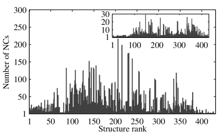
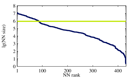
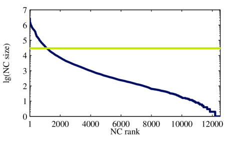
Our system has distinct secondary structures (at a folding temperature of C) of which or about are large. The large structures cover of the folding sequences. By exhaustively searching through all of sequence space, we are able to identify all components, so that there are on average about components per neutral network. Figure 1 shows how these are distributed among the different NNs. The largest number of components is for a relatively infrequent structure ranked th, and only a few small structures have a single NC (the largest has rank 333). We summarise the data in ESM, Tables S1,S2 and Figs. S2,S3. The NCs can be individually ordered, and are even more skewed than the NNs. Overall, NCs (less than ) are larger than average, but together they cover of non-trivial genotype space.
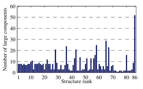
By analogy to NNs we call an NC large if its size is more than the average in its NN. Most NNs contain several large NCs (see ESM, Fig. S4). Rather than being dominated by one NC, we observe that for most phenotypes there are many large NCs. The number of large NCs in an NN is strongly correlated with where is the number of bonds in the corresponding secondary structure (). In contrast, there is hardly any correlation between the number of large NCs and NN size ().
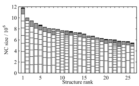
In Figure 2 we show the size of the components for the largest NNs that, together, cover over of the folding genotypes. Most networks have more than the components we expect due to the biophysical argument given above; nonetheless the largest NCs are generally very similar in size, and much larger than all the smaller NCs of the network. Note that the largest NC is for an NN that is ranked th by overall size, and more generally that the size of these largest NNs is not a reliable guide to the average size of the large NCs.
If in addition to the point mutations, we also allow base-pair swaps, then the number of components drops significantly. In particular, as predicted by random graph theory reidys1997percolation , the majority of large NNs are dominated by a single giant NC. This big difference, caused by introducing base pair swaps, strongly suggests that the NN fragmentation we observe under point mutations arises from the simple neutral reciprocal sign epistasis mechanism we identified above.
While single point mutations cannot connect up the NCs, one may consider whether crossover moves may do so. In that context it is helpful to consider Kimura’s analogy to a lock-key system kimura1985compensatory : A change in the lock makes it necessary for the key to be changed accordingly. Crossing over one lock-key setup with another can only be successful in two cases. First, if the lock and key originate from different parents, successful offspring will arise only if the parents are compatible. Second the lock and key may originate from the same parent; this requires that crossover arise at special points in the sequence to ensure a matching lock and key.
In RNA, the first case means that both parental sequences belong to the same NC and that the offspring consequently stay in that NC. The second case is possible only if the point of crossover is outside the looped region of the stem that is incompatible in the parent sequences. This is illustrated in ESM, Fig. S9. Under the second condition, crossover can put offspring onto NCs that are distinct from either parent; however, such crossover only allows to explore a small subset of all possible NCs in an NN. Even this limited exploration is predicated on the population being distributed on multiple NCs in the first place, but this cannot be achieved without compensatory mutations. It is worth noting that crossover slows down the rate of fixation of compensatory mutations kimura1985compensatory .
So far, we have shown that under fairly general conditions, the NNs of RNA secondary structure are fragmented into many NCs. This fact raises the following question: Are the different NCs similar or heterogenous in their properties?
III Neutral components shape evolutionary trajectories
III.1 Robustness increases with component size
The robustness to genetic change has been widely studied in the context of NNs. In particular, van Nimwegen et al. have shown how the robustness of an evolving population depends on the structure of the underlying neutral space vanNimwegen1999robustness . While the dynamic properties of a population depend also on its size and mutation rate, we consider here only the effect of the structure of the NC. To this end, we define the mutational robustness of a genotype as the fraction of mutations that leave the phenotype unchanged. In analogy to wagner2008paradox we calculate the robustness of an NC by averaging the genotypic robustness of all genotypes in the NC. This measure gives the expected average robustness of a monomorphic population evolving on the NC vanNimwegen1999robustness .
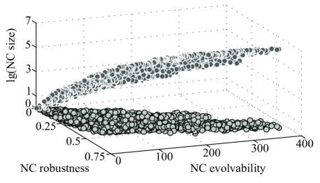
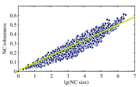
In agreement with earlier results based on sampling techniques wagner2008paradox we observe a clear positive correlation between mutational robustness of an NC and its size (), as illustrated in Fig. 3. Hence, the larger the NC, the more likely individuals are to pass their phenotype on to their offspring after a random mutation. Given the large heterogeneity of NC sizes comprising a given NN, these results suggest that robustness estimates based on the NN as a whole will not be representative of the robustness experienced by a population confined on a given NC. For example, if a population is restricted to a small component of a very large NN, the effective mutational robustness will be (much) lower than that estimated for the NN as a whole.
III.2 Evolvability varies between components of the same phenotype

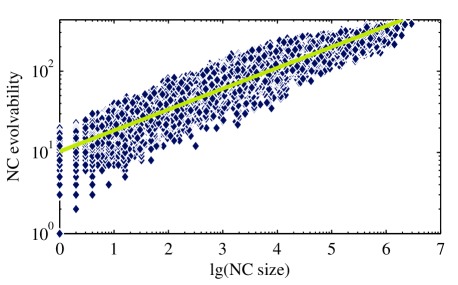
The evolvability of a population is related to its ability to produce heritable phenotypic change pigliucci2008evolvability . One might naively think that the more robust a phenotype is to mutations, the harder it is for mutations to generate novelty. However, this argument ignores the ability of neutral exploration to pave the way for future adaptive innovations wagner2008neutralism . Wagner has proposed a proxy measure of evolvability that counts the number of phenotypes that can be reached by a single mutation from a given NN wagner2008paradox . He showed that this measure also correlates positively with the size of an NN, and argued that phenotypes with larger NN may be simultaneously more robust and more evolvable. But if the NNs are fragmented into separate NCs, then it is in fact the NC robustness and evolvability that matter to a population, and not the properties of the whole NN, which it cannot access by point mutations. Nevertheless, we find that the average robustness and evolvability of individual NCs are positively correlated (Fig. 3, ESM, Figs. S10 and S11) just as was found for NNs. We can thus qualify’s Wagner’s result wagner2008paradox : Robustness and evolvability are not so much correlated at the level of phenotypes (NNs), but rather the correlation holds at the level of an NC (our results yield ), which can vary strongly within one NN.
Thus different populations with the same phenotype may exhibit significantly different evolvabilities. These differences can be further quantified with the following definitions:
| (1) | |||||
| (2) |
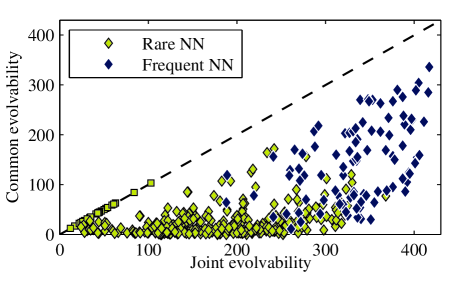
where is the set of phenotypes that can be reached by a single mutation from NC . Thus the joint evolvability (1) counts the number of structures that can be reached from at least one NC in the NN, while the common evolvability (2) counts the structures available from all NCs. The comparison of these two properties reveals significant heterogeneity in the phenotypic neighbourhoods of NCs in the same NN (see Fig. 4a). In fact the joint and common evolvability are only identical for those small NNs that are fully connected. For most NCs, a population will only be able to access a restricted subset of the entire NN’s neighbouring phenotypes: Averaged over all NNs, . There is no significant correlation of and NN size: .
We can further explore this heterogeneity by restricting our analysis to the large NCs only. We expect the differences to diminish because the joint evolvability has a lower bound given by the most evolvable NC while the common evolvability cannot be larger than for the least evolvable NC, which is typically very small. As Fig. 4b shows, the ratio of common to joint evolvability decreases when only large NCs taken into account: with a weak correlation with NN size: . We note that some phenotypes are only accessible from small NCs so the joint evolvability decreases slightly (on average by about ). In ESM, Fig. S12 we restrict the phenotypes further to just those that are large – the same general results hold. Finally, we can ask what fraction of the joint evolvability are accessible on average from a single NC. If we consider only the large NCs of the frequent phenotypes, this fraction is on average (in agreement with cowperthwaite2008ascent ), while averaging over all NCs in all NNs brings this down to (see also ESM, Fig. S13). Instead of requiring large NCs to be greater than the average NC in their NN, we also employed an entropy-based criterion and obtained qualitatively similar results (ESM, Sec. S3.3 and Fig. S14).
It is important to consider whether this discrepancy is an artefact of the relative short sequences we study. Answering this question by exhaustive enumeration is unfeasible. Instead, we employed a sampling technique (ESM, Sec. S4) for sequences of 20 nucleotides. We find that the heterogeneity between NCs becomes even more pronounced as the sequence length increases (ESM, Fig. S15).
Taken together, we have arrived at a key result: the potential for future innovation does not only depend on the current phenotype, but also on which NC a population occupies. The fact that different NCs provide access to different new phenotypes suggests a new mechanism for contingency in evolution. A dynamic setting in which this may be particularly important is a polymorphic population with genotypes from two (or more) NCs. If environmental changes are sufficiently rapid (that is faster than genetic drift), this could drive parts of the population to different phenotypes, potentially aiding diversification at the phenotype level gavrilets2004book .
IV Discussion
We have shown how neutral reciprocal sign epistasis in RNA leads to fragmentation of NNs into multiple components. For many of the NNs, no one component dominates. Moreover, the components are heterogeneous, so that different populations with the same phenotype, but different NCs, may show large variations in robustness and evolvability.
These inferences were possible because of the tractability of the GP map between an RNA sequence and its secondary structure. An obvious question is whether our results extend to other maps. Boldhaus and Klemm boldhaus2010GRNcomponents studied a coarse-grained Boolean threshold dynamics model li2004yeast for the regulatory network of the yeast cell cycle and identified nearly half a billion functional NCs, ranging in size between and genotypes. Interestingly, the wild type network is part of one of the smaller NCs. It contains networks which are quite sparse and noise-resilient, indicating that there are secondary aspects in the performance of the network which can be selected for. This example also shows heterogeneity in the properties of NCs. One caveat is that the point mutations were in an abstract space with discretised interactions. It is not yet clear how a more realistic model of mutations would affect the NCs.
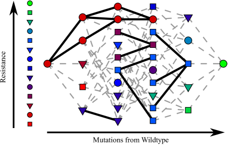
Recent experimental reconstructions of fitness landscapes may also open up avenues to study NCs. For example, in an important paper, Weinreich et al. weinreich2006paths characterized all combinations of mutations that together increase resistance to a particular antibiotic by a factor of about . By measuring the resistance of each possible combination, they produced a phenotype landscape; in examining their data, we found that this landscape also contains several NCs (see ESM, Fig. S16).
There are two important caveats to this finding: First, the resistance scale used in the experiment is relatively coarse. Thus the neutrality in this landscape may even be broken by relatively small populations. In general, we stress that neutrality is always an effective statement, depending on population size ohta1973 .Second, we cannot exclude the existence of neutral connections that were outside the scope of the experiment. Excluding such paths by exhaustively cataloguing all possible mutations would be prohibitive. Progress can be made by studying the biophysics of a GP map, and looking for examples of lock and key type systems. In proteins, binding sites may be potential candidates kimura1985compensatory . However, as reviewed by Poelwijk et al. poelwijk2007landscape , even lock and key systems can sometimes evolve in subtle ways through single mutations.
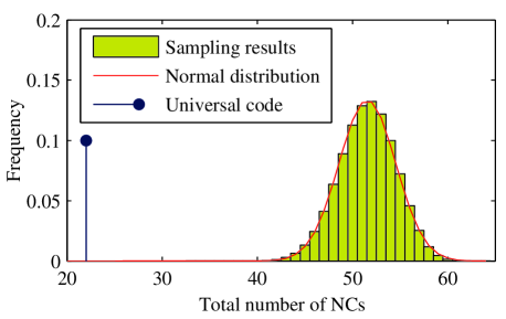
Another system to consider is the genetic code. It is interesting to note that with the exception of serine, all sets of codons coding for a particular amino acid can be reached by single synonymous point mutations. However, serine has two NCs, one made up of AGU and AGC, and the other of UCU, UCC, UCA and UCG. Given that serine often plays a key role in active sites in proteins, it may be that it cannot easily be neutrally replaced by another amino acid, so that these two NCs may indeed be separate in nature. It is noteworthy that this high NN connectivity is extremely unlikely to arise in a random genetic code with the same degeneracy as the universal code (ESM, Fig. S17). As robustness correlates with NC (and not NN) size, this striking degree of NN connectivity may be a by-product of selection for other properties such as robustness of the genetic code to point mutations or translation errors wagner2005book .
We have focussed on the approximation of strong selection and weak mutations where double mutations are excluded. However, compensatory mutations can occur if the fitness penalties are weak, or if mutation rates are high. Measuring fitness is notoriously difficult, but a recent study of compensatory mutations in mitochondrial transfer RNA estimates that transitions from GC to AU may occur through low fitness GU and AC intermediates kondrashov2010RNA . By contrast, switches like AUUA, GCCG and AUCG, each of which requires a transversion, were found to be very rare. These results suggest that in nature we should expect fragmented neutral spaces in RNA to be common.
Nevertheless, a sufficiently large population and/or high mutation rate can lead to a regime in which NCs are effectively connected, so that evolutionary dynamics may be less sensitive to the effects of NN fragmentation. In the opposite limit of small populations and/or mutation rates, the average spread of a population in genotype space can be much smaller than the size of many NCs, implying that the local NC structure becomes more important. For a fixed mutation rate, there will thus be a crossover in the effect of NCs on evolutionary dynamics with increasing population size. More generally, the dependence of of evolvability and neutral space exploration on dynamic parameters is an important issue that we plan to address in a future publication.
Our analysis has only considered the local phenotypic neighbourhood of individual NCs. Over longer evolutionary timescales, populations evolve from one phenotype (and hence NC) to another and traverse the phenotypic landscape. In order to understand the importance of landscape structure on such long timescales, it is necessary to study not only accessible phenotypes, but also the connectivity among NCs, which will be the focus of future studies.
In conclusion then, we have focussed on one striking effect of epistasis on neutral evolution, namely the fragmentation of neutral spaces. The heterogeneity of the resultant NCs is important both conceptually and in practice: Properties such as the robustness and evolvability of an evolving population may not only depend on its phenotype, but also on which NC of that phenotype the population occupies. This sensitivity may lead to contingency in evolution: The evolutionary trajectory of a population depends not only on the occurrence of random mutations, but also on the possible innovations that are available to the NCs it happens upon.
References
- (1) Alberch, P. 1991 From genes to phenotype: dynamical systems and evolvability. Genetica 84, 5–11. (doi:10.1007/BF00123979)
- (2) Kimura, M. 1985 The Neutral Theory of Molecular Evolution. Cambridge, UK: Cambridge University Press.
- (3) Ohta, T. 1973 Slightly deleterious mutant substitutions in evolution. Nature 246, 96–98. (doi:10.1038/246096a0)
- (4) Lunzer, M., Golding, G. B. & Dean, A. M. 2010 Pervasive cryptic epistasis in molecular evolution. PLoS Genet. 6, e1001162. (doi:10.1371/journal.pgen.1001162)
- (5) da Silva, J., Coetzer, M., Nedellec, R., Pastore, C. and Mosier, D.E. 2010 Fitness Epistasis and Constraints on Adaptation in a Human Immunodeficiency Virus Type 1 Protein Region. Genetics 185, 293-303. (doi:10.1534/genetics.109.112458 )
- (6) Hinkley, T., Martins, J., Chappey, C., Haddan, M., Stawiski, E., Whitcomb, J. M., Petropoulos, C. J., & Bonhoeffer, S.2011 A systems analysis of mutational effects in HIV-1 protease and reverse transcriptase. Nat. Genet. 43, 487–489 (doi:10.1038/ng.795)
- (7) Meer, M. V., Kondrashov, A. S., Artzy-Randrup, Y. & Kondrashov, F. A. 2010 Compensatory evolution in mitochondrial tRNAs navigates valleys of low fitness. Nature 464, 279–282. (doi:10.1038/nature08691)
- (8) Romero, P. A. & Arnold, F. H. 2009 Exploring protein fitness landscapes by directed evolution. Nat. Rev. Mol. Cell Biol. 10 866–876, (doi:10.1038/nrm2805)
- (9) Phillips, P. C. 2008 Epistasis — the essential role of gene interactions in the structure and evolution of genetic systems. Nat. Rev. Gen. 9, 855–867. (doi:10.1038/nrg2452)
- (10) Wagner, A. 2008 Neutralism and selectionism: a network-based reconciliation. Nat. Rev. Genet. 9, 965-974. (doi:10.1038/nrg2473)
- (11) Pigliucci, M. 2008 Opinion - Is evolvability evolvable? Nat. Rev. Genet. 9, 75–82. (doi:10.1038/nrg2278)
- (12) Hayden, E. J., Ferrada, E. & Wagner, A. 2011 Cryptic genetic variation promotes rapid evolutionary adaptation in an RNA enzyme. Nature 474, 92–95. (doi:10.1038/nature10083)
- (13) Weinreich, D. M. Watson, R. A. & Chao, L. 2005 Perspective: Sign epistasis & genetic constraint on evolutionary trajectories. Evolution 59, 1165–1174. (doi:10.1111/j.0014-3820.2005.tb01768.x)
- (14) Poelwijk, F. J., Kiviet, D. J., Weinreich, D. M. & Tans, S. J. 2007 Empirical fitness landscapes reveal accessible evolutionary paths. Nature 445, 383–386. (doi:10.1038/nature05451)
- (15) Weinreich, D. M., Delanay, N. F., DePristo, M. A. & Hartl, D. L. 2006 Darwinian Evolution Can Follow Only Very Few Mutational Paths to Fitter Proteins. Science 312, 111–114. (doi:10.1126/science.1123539)
- (16) Poelwijk, F. J., Tanase-Nicola, S., Kiviet, D. J. & Tans, S. J. 2011 Reciprocal sign epistasis is a necessary condition for multi-peaked fitness landscapes. J. Theor. Biol. 272, 141–144. (doi:10.1016/j.jtbi.2010.12.015)
- (17) Schuster, P., Fontana, W., Stadler, P. F. & Hofacker, I. L., 1994 From Sequences to Shapes & Back: A Case Study in RNA Secondary Structures Proc. R. Soc. B 255, 279–284. (doi:10.1098/rspb.1994.0040)
- (18) Kimura, M. 1985 The role of compensatory neutral mutations in molecular evolution. J. Genet. 64, 7–19. (doi:10.1007/BF02923549)
- (19) Pigliucci, M. 2008 Sewall Wright’s adaptive landscapes: 1932 vs. 1988. Biology & Philosophy 23, 591–603. (doi:10.1007/s10539-008-9124-z)
- (20) Gavrilets, S. 1997 Percolation on the fitness hypercube & the evolution of reproductive isolation. J. Theor. Biol. 184, 51–64. (doi:10.1006/jtbi.1996.0242)
- (21) Gavrilets, S. 2004 Fitness landscapes & the Origin of Species. Princeton, NJ: Princeton University Press.
- (22) Hofacker, I. L., Fontana, W., Stadler, P. F., Bonhoeffer, L. S., Tacker, M. & Schuster, P. 1994 Fast folding & comparison of RNA secondary structures. Monatsh. Chemie 125, 167–188. (doi:10.1007/BF00818163)
- (23) Reidys, C. M. & Stadler, P. F. & Schuster, P. 1997 Generic properties of combinatory maps: Neutral networks of RNA secondary structures. Bull. Math. Biol. 59, 339–397. (doi:10.1007/BF02462007)
- (24) Fontana, W. & Schuster, P. 1998 Continuity in Evolution: On the nature of transitions. Science 280, 1451–1455. (doi:10.1126/science.280.5368.1451)
- (25) Fontana, W. 2002 Modeling ‘evo-devo’ with RNA. BioEssays 24, 1164–1177. (doi:10.1002/bies.10190)
- (26) Wagner, A. 2005 Robustness and Evolvability in Living Systems, Princeton, NJ: Princeton University Press.
- (27) Grüner, W., Giegerich, R., Strothmann, D., Reidys, C., Weber, J., Hofacker, I. L., Stadler, P. F. & Schuster, P. 1996, Analysis of RNA sequence structure maps by exhaustive enumeration I. Neutral networks Monats. Chemie 127, 355–374. (doi:10.1007/BF00810881)
- (28) Wagner, A. 2008 Robustness & evolvability: a paradox resolved. Proc. R. Soc. B 275, 91 -100. (doi:10.1098/rspb.2007.1137)
- (29) Cowperthwaite, M. C., Economo, E. P., Harcombe, W. R., Miller, E. L. & Meyers, L. A. 2008 The Ascent of the Abundant: How Mutational Networks Constrain Evolution. PLoS Comp. Bio. 4, e1000110. (doi:10.1371/journal.pcbi.1000110)
- (30) Reidys, C. M. 1997 Randomly induced subgraphs of Generalized n-Cubes. Adv. Appl. Math. 19, 360–377. (doi:10.1006/aama.1997.0553)
- (31) van Nimwegen, E., Crutchfield, J. P. & Huynen, M. 1999 Neutral Evolution of Mutational Robustness, Proc. Nat. Acad. Sci. 96, 9716–9720 (doi:10.1073/pnas.96.17.9716)
- (32) Boldhaus, G. & Klemm, K. 2010 Regulatory networks and connected components of the neutral space. Eur. Phys. J. B 77, 233–237. (doi:10.1140/epjb/e2010-00176-4)
- (33) Li, F., Long, T., Lu, Y., Ouyang, Q. & Tang, C., The yeast cell-cycle network is robustly designed. PNAS 101, 4781–4876. (doi:10.1073/pnas.0305937101)
- (34) Jörg, T., Martin, O. & Wagner, A. 2008 Neutral network sizes of biological RNA molecules can be computed and are not atypically small. BMC Bioinf. 9, 464. (doi:10.1186/1471-2105-9-464)
Electronic Supplementary Material
S1 Introduction
The state space for evolving individuals is genotype space. For DNA (or RNA) sequences of length , genotype space contains discrete points, each one corresponding to a unique sequence. Each point can be linked to one-mutational neighbours which differ from the original genotype at only one nucleotide in the sequence. These connections between genotypes create a generalized hypercube in -dimensional space.
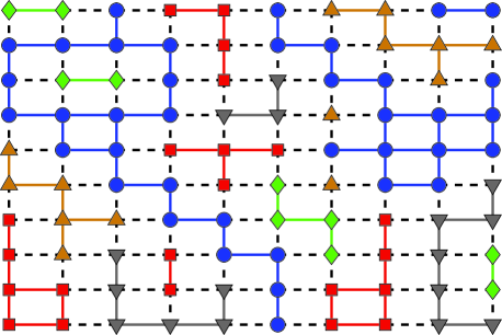
For the purpose of visualisation, we may think of the mapping from genotypes to phenotypes of as a colouring of the hypercube. Then all the vertices (genotypes) with the same colour (phenotype) make up a neutral network (NN). Neutral components (NCs) are sets of genotypes that are connected on the hypercube and share the same phenotype.
It is hard to produce an accurate low-dimensional representation of the genotype hypercube. In Figure S1, we show a simplified picture. It is intended to illustrate the existence of neutral networks and their components. In biologically relevant genotype spaces, the vertices have many more neighbours; in addition, there are no boundaries on the hypercube.
S2 RNA Neutral networks are fragmented
Due to its computational tractability and biological relevance, the folding of RNA sequences into secondary structures is a widely studied GP map schuster1994neutralnetworks ; gruener1996RNAexhaustive ; reidys1997RNAneutralnetworks ; fontana1998continuity ; fontana2002evodevo ; wagner2008paradox ; cowperthwaite2008ascent . In Table S1 we provide data on some well-known characteristics of this map, and the scaling of these properties with sequence length . In particular, the total number of different secondary structures increases exponentially with . Yet this increase is slower than the expansion of sequence space as a whole (which grows as ), so that the average neutral network size also increases with . We compute this average with the trivial structure excluded: this structure is extremely frequent for the short sequences which we study, but it is clear that its abundance decreases quickly as increases.
Figure S2 shows the distribution of NN sizes, by which we just mean the number of genotypes in the respective NN. The size distribution is strongly skewed: A few structures are frequent while most structures are rare. To be precise, we call a secondary structure frequent if its NN is larger than the average NN. Table S1 shows that the absolute number of frequent structures increases with sequence length, while the fraction of structures that are frequent decreases for longer sequences. Nonetheless the fraction of genotypes that map to one of the frequent phenotypes grows with .
In Table S2 we show similar results, focusing on neutral components rather than networks. Just as the number of NNs ( in Table S1) the total number of NCs increases with sequence length. More interesting is the result that the average number of components per network also increases with . It is worth noting that (for the range of we studied here) the mean number of components per network roughly doubles when 2 more bases are added to the sequence. Crudely speaking, two more bases allow to form an extra base pair. This rough argument then agrees nicely with our claim from the main text that the number of NCs can be expected to scale as (where is the number of base pairs in the structure).
While the distribution of NN sizes is heterogeneous (cf. Figure S2), the distribution of NC sizes shows an even more pronounced skew (see Fig. S3). Again defining an NC to be large if it is greater than the average NC, the fraction of large NCs is smaller than the fraction of large NNs. Nonetheless, this smaller proportion of components contains an even larger fraction of genotypes than the large NNs.
Overall, these global considerations indicate a strong heterogeneity in genotype space. Does this heterogeneity also exist within individual NNs? In Figure S4 we show the number of large NCs for all frequent NNs for ; from now on, we call an NC large if it is greater than the average NC in its NN. Almost all frequent NNs contain several large NCs, only the ones ranked 73rd, 74th and 77th are dominated by a single large NC. Overall, for there are 56 NNs with only a single large NC. 19 of these NNs are fully connected. It is clear that all NNs are dominated by their large NCs (Figure S5).
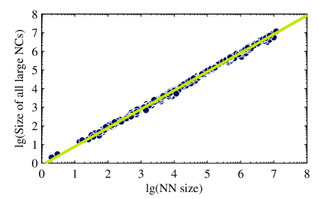
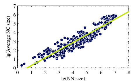
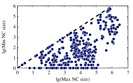
Do larger NNs generally have larger NCs? Figure S6 shows that this is not strictly the case. Of course, the possible NC size is limited by the size of the entire NN. However, the number of NCs in an NN is not strongly correlated with the size of the NN (see main text, Figure 1), but with the number of bonds in the corresponding structure. Therefore, NNs of similar size can have quite different numbers of NCs. Thus the average NC size is not a reliable indicator of the size of the corresponding NN. Additionally, the overall spread in NC sizes in each NN can be very large (Figure S7).
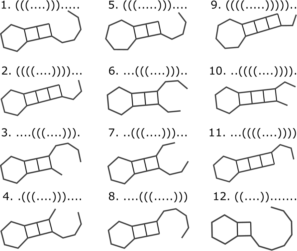
Due to the strong heterogeneity in the number of genotypes per phenotype, the largest NNs are going to dominate genotype space. In Figure S8, we show the 12 most abundant structures; Table S3 lists some of their properties. In particular, the number of (large) components is identical (or close to) , where is the number of base pairs in the structure. For some structures (e.g. the second most abundant one), there are exactly the NCs we expect due to base pair exchanges (see the main paper for details).
This simple dependence of the number of components on the structure corresponding to the NN is striking. In fact, it can be linked to the percolation theory arguments given by Reidys reidys1997percolation . He considers random GP maps and derives a threshold for the average number of neutral neighbour genotypes in order for an NN to percolate. It is clear that the assumption of a random GP map cannot capture the neutral reciprocal sign epistasis that leads to NN fragmentation in RNA. To accommodate for this effect, Reidys introduced another mutational move, namely base pair swaps: In addition to point mutations of individual bases, paired bases are allowed to change in synchrony and thereby maintain a bond.
When we stick with the more restrictive definition of mutations as single nucleotide substitutions, it is still possible to appeal to the percolation theory arguments. However, we need to restrict the set of genotypes to consider. Specifically, given a secondary structure we need to fix for each bond whether the base pair is made in the order purine-pyrimidine, or vice-versa. Thus we take only a subset of all possible genotypes into account. Within this subset, we can expect the percolation argument to be applicable. So if a phenotype is sufficiently frequent (this notion is made precise in reidys1997percolation ), the genotypes mapping into that phenotype will percolate in each separate subspace.
There are also biophysical reasons that may change our expectation of NCs. In particular, our results rest on the assumption that a base pair can be transformed into an pair via a intermediate. Empirically, at our temperature of interest (C) the Vienna package ViennaPackage indicates that neutral intermediates exist, at least in the frequent structures. Nonetheless, it may well be that these intermediates are not neutral in reality. For example, Meer et al. kondrashov2010RNA point out that intermediates of tRNAs may have a strong selective disadvantage. Our simple model in which neutrality is based only on identical secondary structure cannot capture these effects. However, in principle it would be possible to take other factors such as free energy and stability of the native fold into account.
| 1 | 11795379 | 8 | 16 | 8 | 0.53 |
| 2 | 9978003 | 16 | 16 | 8 | 0.67 |
| 3 | 9454721 | 8 | 10 | 8 | 0.68 |
| 4 | 8988572 | 8 | 10 | 7 | 0.58 |
| 5 | 8698911 | 8 | 26 | 8 | 0.49 |
| 6 | 8303219 | 8 | 10 | 7 | 0.57 |
| 7 | 8050101 | 8 | 10 | 7 | 0.56 |
| 8 | 8001910 | 8 | 15 | 8 | 0.46 |
| 9 | 7914436 | 16 | 16 | 8 | 0.56 |
| 10 | 7675391 | 16 | 16 | 10 | 0.69 |
| 11 | 7647918 | 16 | 20 | 11 | 0.31 |
| 12 | 7525506 | 4 | 9 | 3 | 0.15 |
S2.1 Crossover does not provide compensatory mutations
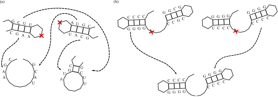
In our construction of the genotype space hypercube, we have only taken point mutations into account when we connected neighbouring genotypes. In nature, other mutational moves are also observed: Deletions or insertions correspond to omitting or adding bases during reproduction of the genotype. These mutations change the sequence length which makes them hard to discuss in our framework.
There is one other kind of mutation that we can address, namely crossover. This mutational move is particularly relevant to sexually reproducing organisms in which the offspring receives part of its genotype from each parent444Asexual organisms such as bacteria can also mutate under crossover by horizontal gene transfer. Can crossover connect separate NCs?
The simplest case to study is when both parental genotypes belong to the same NC. Let us focus on a single base pair for simplicity – if any single pair is not maintained in the offspring phenotype, that phenotype is necessarily different from the parental one. For definiteness, we assume that the base pair of interest is made by a purine-pyrimidine pair in both parents, say GC in one and AU in the other555Having a GC and a GU pair in the same NC is likely to occur only in frequent structures. For rare phenotypes, only GC may exist; this is not important to the argument. Evidently, crossover between the parents will again result in a purine-pyrimidine pair. Depending on the parental base pairs, this could be GC, GU, AU or AC. The first three pairs are compatible and may thus lead to the parental phenotype. However, they will again be part of the same NC – a transition into a pyrimidine-purine pair (which would necessarily be part of a different NC) is not possible. Finally, an AC pair is incompatible and will lead to a different phenotype.
The case of parental genotypes from different NCs is slightly more involved. Let us again consider a purine-pyrimidine pair in the first parent, but now a pyrimidine-purine pair in the other parent. We now need to distinguish two cases depending on the point of crossover. First, consider the case that the crossover point is within the stem-loop region enclosed by the base pair of interest (illustrated in Figure S9a). This means that the resulting genotypes will have either a purine-purine or a pyrimidine-pyrimidine pair, neither of which can form a bond. Thus the offspring phenotype is necessarily different from the parent. Second, the point of crossover may be outside the stem-loop region of interest. In that case, the base pair is left intact. If the parental phenotype contains two separate stem-loop regions, this scenario of crossover may lead to a new NC: Individually incompatible stems are collectively ‘shuffled’. Yet this way of exploring different NCs is limited to reusing the already existing stems; new variants of individual stems cannot be achieved in this manner.
In summary, crossover alone cannot lead to new NCs. In order to create genotypes on an NC that is different from the parental NCs, it is necessary to cross genotypes from different NCs in special positions. However to arrive at a new NC in the first place still requires two mutations even if crossover is taken into account.
S3 Neutral components shape evolutionary trajectories
In the main paper, Fig. 3 we show that the robustness to genetic change and the number of phenotypes in the one-mutant neighbourhood of an NC and its size are correlated. Here, we provide additional views of this data set, focusing on the correlation of robustness and NC size (Figure S10) and on the correlation of evolvability and NC size (Figure S10).
S3.1 Common and joint evolvabilities for large NNs
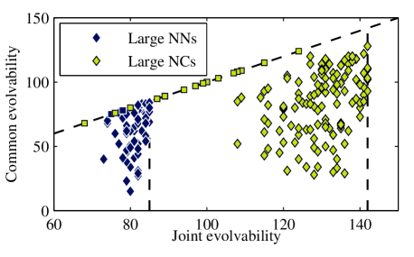
Given the large skew in the size of the NNs, it is worth considering another question regarding joint and common evolvability: Can the large NNs be reached from each other? By only considering the large NCs of the large NNs, we account for NNs and of (non-trivial) genotype space. Alternatively, we can consider all NCs which are larger than the average NC size (calculated from all NCs, not just a particular structure). There are NNs with at least one such NC, and all large NCs together cover of all non-trivially folding genotypes. In both cases, we observe in Fig. S12 that the discrepancy between joint and common evolvability remains significant.
S3.2 Relative evolvability for individual NCs
The common evolvability (as defined in the main text, Eqn. (3)) gives the number of phenotypes that can be reached from any NC in a given NN. This is often much less than the joint evolvability (main text, Eqn. (2)) indicating that there are many phenotypes that can only be reached from some, but not all NCs with a given phenotype. But this does not tell us how many phenotypes can be reached on average from a NC in a given network. To measure this quantity, we define the mean relative evolvability as the ratio of NC evolvability to NN (joint) evolvability, averaged over all NCs in the network. Alternatively, we can restrict the average to the large NCs only. In Figure S13, we show that this fractional evolvability increases slightly with phenotype abundance, but remains clearly below unity. This means that to sample all phenotypes that are part of the joint evolvability, it is necessary for a population to jump between NCs.
If we take the average over all NNs (cf. Figure S13a), we find that the mean relative evolvability is around ; for the frequent NNs, this average is . If we take only large NCs into account (Fig. S13b), the average is for all NNs and for the frequent NNs.

S3.3 Choosing large NCs according to entropy stresses the importance of fragmentation
Our definition of what constitutes a large NC (namely it must be larger than the average NC its NN) is in analogy with we call a frequent phenotype gruener1996RNAexhaustive . An alternative definition can be made in terms of the entropy of the distribution of NC sizes. If we denote the relative size of NC by we have where the sum is over the NCs of a given NN. The entropy of the distribution is then
If the NN in question were fragmented into NCs of equal size, we would obtain and . So gives us an approximate number of NCs whose relative size is significant in the NN. So in order to determine the large NCs in a given NN, we calculate , round to the nearest integer and choose the largest NCs of the NN.
In general, the entropy requirement is less restrictive than choosing the average size as a threshold: For only NNs (with ranks between 80 and 159) the number of large NC is reduced under the entropy criterion (by 1 NC each). For 58 NNs, the number of NCs is the same for both criteria. Thus there remain 367 NNs which have more large NCs by entropy than by average size, and the increase can be up to 5-fold (on average, it is 1.6-fold). In absolute terms, the entropy criterion produces 4 additional large NCs on average.
Regarding the discrepancy between joint and common evolvability, it is clear that a larger number of NCs cannot have a smaller joint evolvability or a bigger common evolvability than a smaller set. So if we consider the joint and common evolvability of the large NCs in an NN, the entropy measure will - for almost all NCs - increase the gap between the two values. This is illustrated in Fig. S14. The ratio of common to joint evolvability, when calculated for the NCs that are large according to the entropy criterion, is when averaged over all NNs. correlates with NN size: , so the discrepancy between joint and common evolvability is less pronounced for large NNs. All these results are quantitatively similar and qualitatively consistent with the average size criterion for large NCs that we have adopted in the main paper.
Given the two different criteria for what constitutes a large NC, is one more appropriate than the other? One advantage of the entropy requirement is that it does not introduce a somewhat arbitrary, hard cutoff. Choosing the average NC size as a threshold means that it is practically impossible to find that all NCs are large - this would arise only if all NC had exactly the same size. It thus appears that the entropy requirement should be favoured. Clearly, this measure is more lenient in that on average it classifies more NCs as being large. As our main interest in this paper is to discern whether the fragmentation of NNs is important for evolutionary dynamics, we have chosen the more restrictive, average-based approach in the main paper. This criterion on average produces less large NCs; thus the effect of fragmentation is less pronounced. Thus the more natural, entropy-based approach suggests that NN fragmentation could be even more severe than outlined in our paper.
S4 Sampling at confirms our results
As genotype space grows exponentially with sequence length, exhaustive enumeration becomes infeasible for longer (and thus biologically more interesting) sequences. In particular, to study the evolvability of NCs we need to explore them completely. For RNA NNs, we can exploit the fact that their fragmentation has a simple cause, namely base pair complementarity. Using this insight, it is relatively straightforward to obtain sequences with the same structure but from different NCs: The Vienna package ViennaPackage includes a function to inverse-fold structures with constraints. Thus we can fix the base pairs and then try to obtain sequences with the desired structure. Using these sequences the NCs of a given NN can be mapped out. The evolvability can be calculated exactly for each NC by simply keeping track of the phenotypes found by non-neutral mutations.
There is no guarantee that this approach will find all NCs; clearly, we are more likely to discover sequences on the large NCs. For computational convenience, we have run the inversion algorithm on sequences for each of the configurations of paired bases (again, is the number of base pairs), choosing the unpaired base uniformly at random for each attempt. We should thus be able to find NCs of sizes ranging over at least orders of magnitude; in fact, this range has turned out much larger, getting up to orders of magnitude. Details of the structures we sampled are given in Tab. S4.
In order to demonstrate that we found most genotypes of an NN, we use the sampling algorithm by Jörg et al. joerg2008NNsize to estimate NN sizes. By comparing the estimated NN size to the number of genotypes found by our sampling approach, we find an indication whether the sampling approach has found all major NCs.
It is important to be clear what it means that smaller NCs may not be found. From the definitions (Eqns. () and () in the main text) it is evident that any subset of NCs gives us a lower bound on the joint evolvability and an upper bound on the common evolvability. Therefore, if the sampling is incomplete, better results can only show that the discrepancy between and is greater than our results indicate.
In general, we find that the discrepancy between joint and common evolvability is large (Fig. S15): on average, and . Therefore, the contingency due to neutral space fragmentation will be important at biologically realistic sequence lengths.
| Structure | Estimated size | Sampled size | NCs | Large NCs | ||
|---|---|---|---|---|---|---|
| ((((....))))........ | 16 | 0.65 | ||||
| .((((....))))....... | 16 | 0.62 | ||||
| ..((((....))))...... | 16 | 0.58 | ||||
| (((((....)))))...... | 32 | 0.70 | ||||
| ...((((....))))..... | 16 | 0.54 | ||||
| ....((((....)))).... | 16 | 0.53 | ||||
| ......(((((....))))) | 32 | 0.28 | ||||
| ...(((((....)))))... | 32 | 0.56 | ||||
| ((((((....)))))).... | 64 | 0.66 | ||||
| ....((((((....)))))) | 64 | 0.30 | ||||
| ..((((((....)))))).. | 64 | 0.65 | ||||
| ..((((((....)).)).)) | 64 | 0.24 | ||||
| ((((..((....))..)))) | 64 | 0.24 | ||||
| ((....))..(((....))) | 32 | 0.08 | ||||
| ((.((.((....))))..)) | 64 | 0.22 | ||||
| (((....)))..((....)) | 32 | 0.13 | ||||
| ((....))....((....)) | 16 | 0.14 | ||||
| ((.((.((....)).)).)) | 64 | 0.10 | ||||
| ((((..((....))))..)) | 64 | 0.04 |

S5 NCs beyond RNA
Establishing the fragmentation of a NN is challenging. If we cannot exploit simple biophysical principles (as in the case of RNA), or if we would like to study properties of NCs, we need to determine phenotypes for large portions of genotype space. Due to the vast numbers of genotypes even in small systems, this is a demanding task. Experimental progress in this area is underway; a pioneering study by Weinreich et al. weinreich2006paths has determined the antibiotic resistance due a particular -lactamase. The authors considered 5 mutations that jointly increase the resistance by about 100,000 fold and measured the resistance of all intermediate mutants between the wildtype and the most resistant type. In Figure S16, we show the resistance landscape that arises in this system. Within the resolution of the experiment, there are several NNs of genotypes that convey the same resistance. Some of these NNs contain multiple NCs; however, it cannot be ruled out that mutations outside the scope of the experiment connect these NCs.
Another system in which the mapping from genotype to phenotype is well characterized is the genetic code, linking triplets of nucleotides in DNA (or mRNA) to amino acids in proteins666In many other contexts, the sequence of residues in a protein is considered as its genotype. Fundamentally however, mutations change DNA, while biological function depends on the amino acid sequence.. Here, a neutral network consists of all the codons that are translated into the same amino acid (we treat the STOP signal as another amino acid). In the universal genetic there are 21 NNs with sizes between 6 (arginine, leucine, serine) and 1 (methionine, tryptophan). Serine is the only amino acid whose NN is fragmented. This NN contains NCs which have size 2 and 4, respectively. So in total, there are 22 NCs in 21 NNs.
It is well known that the universal genetic code is significantly different from an arbitrary assignments of codons to amino acids wagner2005book . Here, we are interested to discern if the NN connectivity observed in the code is another property that sets the universal code apart from a random alternative. To this end, we generated codes by assigning each codon a randomly chosen amino acid, such that the degeneracy of the universal code is maintained. For each realization, we counted the overall number of NCs. A histogram of the data is shown in Figure S17. On average, a random code contains NCs, much more than the 22 NCs of the universal code. The lowest number of NCs in our sample was 33 and this was realized only once. The maximum possible number of NCs, 64, was found in 23 random realizations of the code.
It is clear that the degree of NN connectivity of the universal code is far from random. However, the universal code does not minimize the total number of NCs completely – for example, exchanging the 2 tyrosine codons with the smaller NC of serine would yield a maximally connected code. One possible explanation of the high connectivity of the universal code is that it confers robustness of the protein amino acid sequence to point mutations in the DNA and to translation errors wagner2005book . This finding illustrates an important message of the main paper: The robustness of a phenotype (the amino acid) cannot be ascribed to the properties of phenotype itself (such as the degeneracy of the amino acid), but is sensitive to the local connectivity of the NC.
