The Sherrington-Kirkpatrick model near ${\bm{T}_{c}}$ and near ${\bm{T}=0}$

Abstract

Some recent results concerning the Sherrington-Kirkpatrick model are reported. For $T$ near the critical temperature $T_{c}$, the replica free energy of the Sherrington-Kirkpatrick model is taken as the starting point of an expansion in powers of $\delta Q_{ab}=(Q_{ab}-Q_{ab}^{\rm RS})$ about the Replica Symmetric solution $Q_{ab}^{\rm RS}$. The expansion is kept up to $4$-th order in $\delta{\bm{Q}}$ where a Parisi solution $Q_{ab}=Q(x)$ emerges, but only if one remains close enough to $T_{c}$.

For $T$ near zero we show how to separate contributions from $x\ll T\ll 1$ where the Hessian maintains the standard structure of Parisi Replica Symmetry Breaking with bands of eigenvalues bounded below by zero modes. For $T\ll x\leq 1$ the bands collapse and only two eigenvalues, a null one and a positive one, are found. In this region the solution stands in what can be called a droplet-like regime.

1 Introduction

The Sherrington-Kirkpatrick (SK) model [1, 2], introduced in the middle of 70’s as a mean-field model for spin glasses, has played and important role besides the study of spin glasses. The search for its solution in the low temperature phase, the spin glass (SG) phase, has lead to the introduction and development of tools such as the Replica Method and the concept of Replica Symmetry Breaking, that have found applications in a variety of other fields of the complex-system world, just to cite a few, neural networks, combinatorial optimization and glassy physics.

The signature of the SG state is the presence of a large number of degenerate, locally stable states. When the system is driven into the SG phase, the spins almost freeze and fluctuate along local fixed directions. Thus, similar to what happens in the low temperature phase of a ferromagnet, the thermal average of a single spin does not vanishes in the SG phase. Yet, at difference with a ferromagnet, the local directions may change from spin to spin without any special rule, that is in a random way. Therefore the SG phase is not characterized by a long range ordering. Also, since each spin can choose among different local directions, the SG phase is actually made by a large number of degenerate locally stable states. If we take a shot of one of such SG state, we shall discover that it is not distinguishable from a paramagnetic, i.e., disordered state. Thus we can think of the SG phase made by a large set of almost frozen paramagnetic (disordered) states.

Direct consequence of such a scenario is that identical ideal replicas of the system, indistinguishable in the paramagnetic phase, when driven into the SG phase may end up into different SG states and, hence, becoming distinguishable. The symmetry among replicas is then broken.

The solution of the SK model which accounts for this scenario was found at the end of the 70’s, and it is now know as the “Parisi Solution” [3, 4]. Since then many of its properties have been studied and understood. Some questions, however, are still open, among them its validity for finite dimensional systems. Despite the subtleties, and mathematical ambiguities, of the replica method, see e.g. [5], it is now accepted that the Parisi Solution is correct for the mean-field SK model. For finite dimensional systems it is less clear and a different scenario, the droplet picture, an essentially replica symmetric description, as been put forward. The connection between the two is still not fully understood.

In this paper we shall discuss SK model replica symmetry breaking solutions that are obtained by expanding about the replica symmetric solution. The interest for these solutions is twofold: from one side one can investigate the set up of the replica symmetry breaking in the SG phase. The study of these solutions is also relevant for the definition of a field theory description of the SG phase that could be used to investigate the crossover from mean-field to the finite dimensional systems.

In the last part of the paper we shall briefly discuss the solution of the SK model in the limit $T\ll 1$, where an (almost) replica symmetric description arises.

2 The SK model and the SK-solution

The Sherrington-Kirkpatrick (SK) model in absence of external fields is defined by the Hamiltonian [1, 2]

$${\cal H}=-\frac{1}{2}\sum_{i\not=j}^{1,N}\,J_{ij}\,\sigma_{i}\sigma_{j}$$ (1)

where $\sigma=\pm 1$ are Ising spins and the symmetric couplings $J_{ij}$ are i.i.d. quenched Gaussian random variables of zero mean and variance equal to $1/N$. All pairs of spins $(i,j)$ interacts, and the scaling of the variance ensures a well defined thermodynamic limit as $N\to\infty$.

The thermodynamic properties of the model are obtained from the free energy (density) $-\beta Nf_{J}=\ln Z_{J}$, where $\beta=1/T$ is the inverse temperature. In disordered systems $Z_{J}$, and hence $f_{J}$, is a random quantity. We must therefore average the free energy $f_{J}$ over the disorder. To overcome the difficulties of averaging a logarithm, the average over the disorder is computed using the so-called replica trick. This procedure is essentially the identity

$$-\beta Nf=\left[\ln Z\right]_{J}=\lim_{n\to 0}\frac{\left[Z^{n}\right]_{J}-1}{n},$$ (2)

where the square brackets denote disorder average, and $f$ the disorder averaged free energy density. For an integer $n$, $Z^{n}$ may be expressed as $Z^{n}=\prod_{a=1}^{n}Z_{a}$, and may be interpreted as the partition function of $n$ identical, non-interacting, replicas of the real system. Averaging $Z^{n}$ for integer $n$ over disorder introduces an effective interaction between replicas. Performing the average, and introducing the auxiliary symmetric replica overlap matrix $Q_{ab}=\frac{1}{N}\sum_{i}\sigma_{ia}\sigma_{ib}$, with $a\not=b$, the disordered averaged replica partition function can be written as [2]:

$$\left[Z^{n}\right]_{J}=\int\prod_{a<b}\sqrt{\frac{N\beta^{2}}{2\pi}}\,dQ_{ab}\,e^{N{\cal L}[{\bm{Q}}]}$$ (3)

with the effective Lagrangian (density)

$${\cal L}[{\bm{Q}}] = -\frac{\beta^{2}}{4}\sum_{ab}Q_{ab}^{2}+\Omega[{\bm{Q}}]-n\frac{\beta^{2}}{4}$$ (4)

$$\Omega[{\bm{Q}}] = \ln{\rm Tr}_{\sigma_{a}}\exp\bigg{(}\frac{\beta^{2}}{2}\sum_{ab}Q_{ab}\,\sigma_{a}\sigma_{b}\bigg{)}$$ (5)

The last term in (4) follows from the definition $Q_{aa}=1$. The normalization factor in (3) gives a sub-leading contributions for $N\to\infty$ and is omitted in the following.

In the thermodynamic limit, $N\to\infty$, the integral over $Q_{ab}$ in (3) is evaluated at the stationary point,

$$\frac{\partial}{\partial\,Q_{ab}}\,{\cal L}[{\bm{Q}}]=0,\quad a<b,$$ (6)

that leads to the self-consistent equation for $Q_{ab}$:

$$Q_{ab}=\frac{{\rm Tr}_{\bm{\sigma}}\sigma_{a}\sigma_{b}\,\exp\left(\frac{\beta^{2}}{2}\sum_{ab}Q_{ab}\right)}{{\rm Tr}_{\bm{\sigma}}\exp\left(\frac{\beta^{2}}{2}\sum_{ab}Q_{ab}\,\sigma_{a}\sigma_{b}\right)}=\langle\sigma_{a}\sigma_{b}\rangle,\qquad a\not=b.$$ (7)

The replica free energy density then reads:

$$-n\beta\,f(n)={\cal L}[{\bm{Q}}],$$ (8)

and the average free energy $f$ is recovered as the limit $n\to 0$ of $f(n)$.

To solve the self-consistent stationary point equation (7) an assumption on the structure of the overlap matrix $Q_{ab}$ must be done. As the $n$ replicas of the real system are identical, one may reasonably assume that the solution should be symmetric under the exchange of any pair of replicas. Based on this, SK in their original work assumed [2]

$$Q_{ab}=\delta_{ab}+q\,(1-\delta_{ab})$$ (9)

where $q$ is the overlap between any pair of different replicas. This form of $Q_{ab}$ is what it is now known as the Replica Symmetric (RS) Ansatz. The physical meaning of $q$ is

$$q=\left[\langle\sigma_{i}\rangle^{2}\right]_{J}$$ (10)

where $\langle\cdots\rangle$ denotes here thermal average for fixed disorder. In absence of an external field the local direction of $\langle\sigma_{i}\rangle$ is random, and depends on the disorder realization, and hence $\left[\langle\sigma_{i}\rangle\right]_{J}=0$. Therefore a nonzero $q$ indicates local magnetic order, without a long range ordering.

Substitution of Ansatz (9) into the stationary point equation (7), or into eqs. (4), (5) and (6), leads in the $n\to 0$ limit to the self-consistent equation

$$q=\int_{-\infty}^{+\infty}\frac{dz}{\sqrt{2\pi q}}\ e^{-z^{2}/2q}\,\tanh^{2}(\beta z),$$ (11)

that, besides the paramagnetic solution $q=0$, admits for $T<T_{c}=1$ a non-trivial $q\not=0$ solution. The order parameter $q(T)$ is a decreasing function of temperature, that is equal to $1$ at $T=0$ and vanishes for $T\to T_{c}^{-}$. An explicit solution of (11) may be obtained by expanding near the points $T=0$ and $T=1$. One then finds that $q$ vanishes as $T_{c}-T$ as the critical temperature $T_{c}$ is approached from below, while $1-q(T)\sim T$ as $T\to 0$.

This solution yields, however, an unphysical negative zero temperature entropy [2]. The analysis of the stability of the stationary point also reveals that the RS stationary point becomes unstable as $n\to 0$ for all temperatures $T<T_{c}$ [6].

The failure of the RS Ansatz has a physical origin. Below the critical temperature $T_{c}$ the phase space of the SK model breaks down into a large, yet non extensive, number of degenerate locally stable states in which the system freezes. The symmetry under replica exchange is then spontaneously broken, and the overlap matrix becomes a non-trivial function of the replica indexes. Following the parameterization introduced by Parisi [3, 4], the overlap matrix $Q_{ab}$ for $R$ steps of replica permutation symmetry breaking –called RSB solution– is divided along the diagonal into successive boxes of decreasing size $p_{r}$, with $p_{0}=n$ and $p_{R+1}=1$, and elements given by:

$$Q_{ab}\equiv Q_{a\cap b=r}=Q_{r},\qquad r=0,\cdots,R+1$$ (12)

with $1=Q_{R+1}\geq Q_{R}\geq\cdots\geq Q_{1}\geq Q_{0}$. In this notation $r=a\cap b$ denotes the overlap between the replicas $a$ and $b$, and means that $a$ and $b$ belong to the same box of size $p_{r}$ but to two distinct boxes of size $p_{r+1}<p_{r}$.

The solution of the stationary point equation can be obtained for any value of $R$ [3, 4, 7]. The case $R=0$ gives trivially back the RS solution. It turns out that a physically acceptable solution for the SK model is obtained only by letting $R\to\infty$, that is by allowing for an infinite number of possible spontaneous breaking of the replica permutation symmetry. The solution is called full replica symmetry breaking (FRSB), or infinite-RSB solution ($\infty$-RSB) to stress the limit $R\to\infty$. In this limit $Q_{r}-Q_{r-1}\to 0$, $r=0,\ldots,R$, and the matrix $Q_{ab}$ is described by a continuous, non-decreasing function $Q(x)$ parameterized by a variable $x$. The meaning of $x$ may depend on the parameterization used. In the Parisi scheme $x\in[0,1]$ and measures the probability for a pair of replicas to have an overlap not larger than $Q(x)$ [8]. The FRSB equations can be solved in the full low temperature phase [9, 10, 11, 12, 13, 14, 15]. In Fig. 1 we show the form of $Q(x)$ obtained from the numerical solution of the FRSB equation [From Ref. [10]].

Figure 1: $Q(x)$ as function of $x$ for various temperatures. From bottom to top $T=0.95$ to $T=0.30$ in step of $0.05$ [From Ref. [10]].

3 Expansion around the RS solution

From the analysis of the replica symmetry breaking solution at small finite replica number $n$, Kondor [16] has found that below, but close to, the critical temperature $T_{c}$ the instability of the RS solution appears at the finite value $n=n_{s}(T)<1$. For $n\geq n_{s}(T)$ the free energy $f(n)$ coincides with $f_{\rm SK}(n)$ from the RS solution, while for $0\leq n\leq n_{s}(T)$ it is given by $f_{\rm FRSB}(n)$ from the FRSB solution. The crossover is rather smooth since $f_{\rm SK}(n)$ and $f_{\rm FRSB}(n)$, along with their first two derivatives, coincide at $n_{s}(T)$. To investigate the nature of the replica symmetry breaking in the low temperature phase one can then expand $Q_{ab}$ around the RS solution.

One then considers an overlap matrix $Q_{ab}$ of the form, see eq. (9),

$$Q_{ab}=Q_{ab}^{\rm RS}+q_{ab}=\delta_{ab}+q\,(1-\delta_{ab})+q_{ab}$$ (13)

where $q$ is given by the SK Replica Symmetric solution (11) and $q_{ab}$ is the deviation from the Replica Symmetric solution. Inserting this form of $Q_{ab}$ into (4), and expanding the functional $\Omega[{\bm{Q}}]$ in powers of $q_{ab}$, yields:

$$-n\beta f=-n\beta f_{\rm SK} - \frac{\beta^{2}}{2}q\sum_{ab}q_{ab}-\frac{\beta^{2}}{4}\sum_{ab}q_{ab}^{2}$$ (14)

$$+ \sum_{k\geq 1}\frac{1}{k!}\left(\frac{\beta^{2}}{2}\right)^{k}\left\langle\left(\sum_{ab}q_{ab}\,\sigma_{a}\sigma_{b}\right)^{k}\right\rangle_{c}+O(n^{2})$$

where the subscript “$c$” indicates that only connected contributions must be considered, i.e., only the terms that cannot be written as the product of two or more independent sums. All others give contributions of $O(n^{2})$, or higher. The first contribution, $f_{\rm SK}$, is the SK free energy

$$-\beta f_{\rm SK}=\frac{\beta^{2}}{4}q^{2}-\frac{\beta^{2}}{2}q+\overline{\ln\cosh(\beta z)}+\ln 2+O(n)$$ (15)

where the overbar denotes the average over the Gaussian variable $z$:

$$\overline{g(z)}=\int_{-\infty}^{+\infty}\frac{dz}{\sqrt{2\pi q}}\ e^{-z^{2}/2q}\,g(z).$$ (16)

Whit this notation the RS solution (11) takes the compact form

$$q=\overline{\theta^{2}},\qquad\theta\equiv\tanh(\beta z).$$ (17)

Expanding the cumulants in eq. (14) up to order $O(q_{ab}^{4})$ included, the lowest term needed to break replica symmetry, one obtains [17]

$$-n\beta f = -n\beta f_{\rm SK}+\frac{1}{4T^{4}}\left[M\,\sum_{abc}q_{ac}q_{cb}+N\,\sum_{ab}q_{ab}^{2}\right]$$

$$+\frac{1}{6(2T^{2})^{3}}\left[P\,\sum_{abcd}q_{ac}q_{cd}q_{db}+Q\,\sum_{abcd}q_{ad}q_{bd}q_{cd}+R\,\sum_{abc}q_{ac}^{2}q_{cb}\right.$$

$$\hskip 156.49014pt\left.+J\,\sum_{ab}q_{ab}^{3}+K\,\sum_{abc}q_{ac}q_{cb}q_{ba}\right]$$

$$+\frac{1}{24(2T^{2})^{4}}\left[-A\,\sum_{abcde}q_{ae}q_{be}q_{ce}q_{de}+B\,\sum_{abcd}q_{ac}q_{cd}^{2}q_{db}\right.$$

$$\hskip 42.67912pt-B\,\sum_{abcde}q_{ac}q_{dc}q_{ce}q_{eb}+C\,\sum_{abc}q_{ac}q_{cb}^{2}q_{ba}-C\,\sum_{abcd}q_{ac}q_{ad}q_{dc}q_{cb}$$

$$\hskip 42.67912pt+4D\,\sum_{abc}q_{ac}^{3}q_{cb}-3D\,\sum_{abcd}q_{ab}^{2}q_{bc}q_{bd}+E\,\sum_{abcde}q_{ab}q_{bc}q_{cd}q_{de}$$

$$\left.-2E\,\sum_{abcd}q_{ab}q_{bc}q_{cd}^{2}+F\,\sum_{abcd}q_{ab}q_{bc}q_{cd}q_{da}+G\,\sum_{ab}q_{ab}^{4}-H\,\sum_{abc}q_{ac}^{2}q_{cb}^{2}\right]$$

$$+O(n^{2})$$

where

$$M=2\,\overline{\theta^{2}(1-\theta^{2})},\quad N=\overline{(1-\theta^{2})^{2}}-T^{2}.$$ (19)

$$P=24\,\overline{\theta^{2}(1-\theta^{2})^{2}},\quad Q=-16\,\overline{\theta^{4}(1-\theta^{2})},\quad R=-48\,\overline{\theta^{2}(1-\theta^{2})^{2}},\quad$$ (20)

$$J=16\,\overline{\theta^{2}(1-\theta^{2})^{2}},\quad K=8\,\overline{(1-\theta^{2})^{3}}$$ (21)

$$A=32\,\overline{\theta^{4}(1-3\theta^{2})(1-\theta^{2})},\quad B=384\,\overline{\theta^{4}(1-\theta^{2})^{2}},\quad C=384\,\overline{\theta^{2}(1-\theta^{2})^{3}},$$ (22)

$$D=64\,\overline{\theta^{2}(1-3\theta^{2})(1-\theta^{2})^{2}},\quad E=192\,\overline{\theta^{2}(1-\theta^{2})^{2}},\quad F=48\,\overline{(1-\theta^{2})^{4}},$$ (23)

$$G=32\,\overline{(1-3\theta^{2})^{2}(1-\theta^{2})^{2}},\quad H=96\,\overline{(1-3\theta^{2})(1-\theta^{2})^{3}}.$$ (24)

The equation for $q_{ab}$ follows from the stationarity condition $(\partial/\partial q_{ab})f=0$ applied to the replica free energy functional (3). In the limit $R\to\infty$ this becomes an integro-differential equation for $q(x)$, whose solution is

$$q(x)=\Gamma\frac{x-s}{\sqrt{(x-s)^{2}+\Delta}}-a-bS_{1},\qquad 0\leq x\leq x_{c},$$ (25)

and $q(x)=q(x_{c})$ for $x_{c}\leq x<1$. The parameters $a$, $b$, $s$ and $\Delta$ are functions of the coefficients of the expansion (3), and hence of $T$, while $\Gamma$, $S_{1}$ and $x_{c}$ must be determined selfconsistently. For details we refer to Ref. [17]. It turns out that below the temperature $T=0.549\ldots$ no physical solution with $q(x)\not=0$ is exists and only the SK solution $Q(x)=q$ survives. Figure 2 shows the solution $Q(x)=q+q(x)$ for $T=0.9$.

Figure 2: $Q(x)$ versus $x$ at temperature $T=0.9$. The horizontal dashed line shows the SK solution $Q(x)=q$. For this temperature we have $x_{c}=0.168846\ldots$, $Q(x_{c})=0.109238\ldots$ $Q(0)=0.013570\ldots$ and $q=0.102701\ldots$.

Near the critical temperature $T_{c}=1$ the solution can be expanded in powers of $\tau=T_{c}-T\ll 1$. The first terms of the expansion of $q(x)$ for $0\leq x\leq x_{c}$ read

$$q(x) = \frac{x}{\sqrt{4+6x^{2}}}+\left[1-\frac{4\sqrt{2}}{(2+3x^{2})^{3/2}}+\frac{3x(2+x^{2})}{\sqrt{2}(2+3x^{2})^{3/2}}\right]\,\tau$$ (26)

$$+\frac{1}{3(2+3x^{3})^{5/2}}\Bigl{[}64\sqrt{2}-236\sqrt{2}x+312\sqrt{2}x^{2}-138\sqrt{2}x^{3}-81\sqrt{2}x^{5}$$

$$\phantom{=======}-56\sqrt{2+3x^{2}}-168x^{2}\sqrt{2+3x^{2}}-126x^{4}\sqrt{2+3x^{2}}\Bigr{]}\,\tau^{2}$$

$$+O(\tau^{3}),$$

while for the breaking point $x_{c}$ one has

$$x_{c}=2\tau-4\tau^{2}+\frac{40}{3}\tau^{3}-\frac{665}{9}\tau^{4}+\frac{68567}{135}\tau^{5}+O(\tau^{6}).$$ (27)

From these expressions, and the expansion of the RS solution $q$ close to $T_{c}$, follows

$$Q(0)=q+q(0)=\frac{56}{3}\tau^{3}-\frac{220}{3}\tau^{4}+\frac{3968}{9}\tau^{5}+O(\tau^{6})$$ (28)

$$Q(x_{c})=q+q(x_{c})=\tau+\tau^{2}-\tau^{3}+\frac{5}{2}\tau^{4}-\frac{413}{90}\tau^{5}+O(\tau^{6}).$$ (29)

A peculiarity of this FRSB solution is that $Q(x)$ does not vanishes at $x=0$, as Fig. 2 clearly shows. $Q(x=0)$ only vanishes at $T_{c}$, and grows as $(T_{c}-T)^{3}$, see eq. (28), below it. The reason for such a behaviour is that the FRSB “opens” around the RS solution $Q^{{\rm RS}}(x)=q$. As the temperature decreases the RS solution $q$ grows from zero and drags $Q(x=0)$ to finite values. At $T=0.618\ldots$ the value of $Q(x=0)$ eventually overcomes that of $q$.

In the absence of external fields that break the up/down symmetry $Q(x=0)$ must vanish. The finite value of $Q(x=0)$ then indicates that more terms in the expansion (14) must be retained in order to balance the drag from $q$. Alternatively a null value of $Q(x=0)$ can be recovered by taking $q=0$, which eliminates the drag from the beginning. Physically this means by performing the expansion around the paramagnetic solution. In this case, however, the FRSB solution exists in a narrower region, $0.9148\ldots\leq T\leq 1$, close to the critical temperature.

We note that the choice $q=0$ was used to derive the so called Truncated Model [3, 18] largely used to study the low temperature phase of the SK model. This model is based on an expansion that retains only the main mathematical structure of the expansion of the replicated free energy in powers of $Q_{ab}$ near $T_{c}$, where $|Q_{ab}|\ll 1$, but, similar to the Landau Lagrangian, with arbitrary coefficients. The mapping between the expansion (3) with $q=0$ and the Truncated Model is $F=H=0$, $N=2T^{3}(1-\tau)$, $K=8T^{5}w$ and $G=32T^{7}u$ with arbitrary $u$ and $w$. In this case, if $w$ and $u$ are temperature independent, the FRSB solution exists only down to $T_{\rm trm}=1-w^{2}/4u$.

4 Solution near $T=0$

In the previous Section we have seen that the RS solution can be taken as a starting point for a development of the FRSB solution for $T_{c}-T\ll 1$. As the temperature becomes significantly lower than $T_{c}$ the expansion looses physical meaning and more and more terms are needed into the expansion to extend its validity. Due to the particular structure of the expansion, in powers of $\beta$, it is likely that an infinite subset of terms should be considered to tackle with very low temperatures.

Surprisingly a Replica Symmetric description appears at $T\to 0$. Indeed as the temperature is lowered towards $T=0$ the probability that $Q_{ab}\leq q_{c}(T)=O(1)$ remains finite, viz. $x_{c}\simeq 0.524\ldots$ as $T\to 0$ [19, 10] . At the same time the probability of finding overlaps $Q_{ab}$ significantly smaller than $q_{c}(T)=O(1)$ vanishes with $T$. Then, since $Q(x=0)=0$, for $T\ll 1$ the order parameter function $Q(x)$ undergoes an abrupt and rapid change of $O(1)$ in a tiny boundary layer of thickness $\delta\sim T$ close to $x=0$, while it is slowly varying for $\delta\ll x\leq x_{c}$, as depicted in Fig. 3.

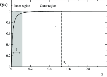
Figure 3: Shape of $Q(x)$ as function of $x$ for $T\ll 1$. The shaded ares shows the extent of the layer of thickness $\delta\sim T$ where the larger variation of $Q(x)$ is concentrated.

In the limit $T\to 0$ the thickness $\delta\sim T\to 0$, and the order parameter function becomes discontinuous at $x=0$.

Uniform approximate solutions valid for $T\ll 1$ can be constructed by studying the problem separately inside (inner region) and outside (outer region) the boundary layer.

The inner solution for $Q(x)$ was first computed by Sommers and Dupont [9], and recently extensively studied by Oppermann, Sherrington and Schmidt [13, 15, 14]. It turns out that as $T\to 0$ the inner solution $Q(a)$ remains a smooth function the inner variable $a=x/T$, needed to blow up the inner region, varying between $0$, for $a=0$, and $q_{c}(T)\sim 1$, for $a\gg 1$. The outer solution was studied by Pankov [12], who found that in the outer region one has

$$Q(x)\sim 1-c(\beta x)^{-2},\qquad T\ll x\ll x_{c}\ \mbox{\rm and}\ T\to 0$$ (30)

where $c=0.4108\ldots$ and $x_{c}\simeq x_{c}(T=0)=0.524\ldots$.

This behaviour of $Q(x)$ has strong consequences on other relevant quantities and, also, on the structure of the eigenvalue spectrum of the Hessian of the fluctuations governing the stability of the stationary point. For what concerns the stability one finds [20, 7] that in the region $x\leq\delta\sim T$, where $Q(x)$ varies rapidly from $0$ up to $q_{c}\simeq 1$, the spectrum of the Hessian of the fluctuations maintains the complex structure of the FRSB solution found close to $T_{c}$ [21]. That is a Replicon band whose lowest eigenvalues are zero modes, and a Longitudinal-Anomalous band of positive masses.

In the region $T\ll x\leq x_{c}$, the eigenvalue spectrum has a completely different aspect. The bands observed in the FRSB regime collapse and only two distinct eigenvalues are found: a null one and a positive one [20]. This ensures that the FRSB solution remains stable down to zero temperature. We note that zero modes arise from the Replicon geometry, with Ward-Takahashi identities protecting them [22], and arises also from the Longitudinal-Anomalous geometry, without protection of the Ward-Takahashi identities. It is worth to observe that the stability analysis of the RS solution also leads to two eigenvalues, one of which is zero to the lowest order in $T_{c}-T$ (and negative to higher order) and a positive one [6].

From the expression (30) it follows that the variation of $Q(x)$ in the outer region, $T\ll x\leq x_{c}$, is $[Q(x_{c})-Q(x)]/Q(x)\sim c(T/x)^{2}$, rather weak for $T\to 0$. Thus in this region, that covers the overwhelming part of the interval $0<x<1$ for $T\to 0$, we have a marginally stable (almost) Replica Symmetric solution, that become a genuine Replica Symmetric solution for $T\to 0$, with self-averaging trivially restored.

5 Discussion

In this paper we have reported some recent results on the solution of the SK model. In particular we have considered two different issues. In the first part we discussed the analysis of the Replica Symmetry Breaking done through an expansion around the Replica Symmetric solution. In the second part we examined the properties of the solution in the limit of vanishing temperature.

The expansion of the replica free energy functional around the RS solution, truncated to the fourth order in $q_{ab}=Q_{ab}-Q_{ab}^{\rm RS}$, leads to a FRSB solution with a continuous order parameter $Q(x)$ below the critical temperature $T_{c}=1$. The solution, however, exists only in the range $0.549\ldots\leq T\leq T_{c}$. Moreover the value of $Q(x=0)$ is finite and vanishes only for $T\to T_{c}^{-}$ with the third power of the temperature difference. A null $Q(x=0)$ can be recovered by expanding about the (replica symmetric) paramagnetic solution $q=0$. In this case, however, the FRSB solution exists only close to $T_{c}=1$, in the narrower interval $0.915\ldots\leq T\leq T_{c}=1$.

For what concerns the stability we believe that the solution form the expansion around the paramagnetic solution $q=0$ has the same stability properties in the most dangerous sector, i.e., in the Replicon subspace by virtue of the Ward-Takahashi identities [22], of the Truncated Model. We believe that this feature remains true for the expansion around the SK solution as well [23]. Thus the FRSB, where it does exist, is marginally stable with null Replicon eigenvalues.

Finite RSB solutions, or even RS solution $q_{ab}=q\,(1-\delta_{ab})$, may also exists. These may exists for all temperatures below $T_{c}$, or only in a limited range of temperature. In either case all these solutions are unstable, with negative Replicon eigenvalues.

The main limitation of the expansions discussed here is the limited range of temperatures where the FRSB solution exists. To extend the range one should retain more terms in the expansion. This will also cure the finite value of $Q(x=0)$. Due to the particular structure of the expansion, in powers of $\beta$, it is likely that an infinite subset of terms should be considered to extend the validity of the expansion to very low temperatures. If one is interested into these temperatures different approaches, e.g., that proposed in Ref. [24] based upon an expansion around a spherical approximation that leads instead to an expansion in $T$, may be more suitable.

The striking property of the solution of the SK model for $T\ll 1$ is the presence of two well distinct regions where the order parameter function $Q(x)$ behaves differently. In the first region, close to $x=0$, $Q(x)$ varies rapidly from $Q(x=0)=0$ to $Q(x)\sim q_{c}=O(1)$ for $x\sim T$. In this region, that contains (almost) the whole variation of $Q(x)$, the solution maintains the structure of the FRSB solution found for higher temperature and close to $T_{c}$, including the complex Hessian spectrum, even in the limit $T\to 0$. For this reason this region was called the RSB-like regime.

In the second region, for $T\ll x\leq x_{c}\simeq=0.575\ldots$, $Q(x)$ is a very slow varying function of $x$, the variation being indeed of the order $[Q(x_{c})-Q(x)]/Q(x)={\cal O}\left((T/x)^{2}\right)$. Here the bands observed in Hessian spectrum for the RSB regime disappear, and only two distinct eigenvalues are found: a null one and a positive one, ensuring the stability of the FRSB solution down to $T\to 0$. In this region, that covers the overwhelming part of the interval $0<x<1$ for $T\ll 1$, the solution strongly resembles a stable RS solution typical of a droplet description. For this reason this region was called droplet-like regime.

In the limit $T\to 0$ the domain of the RSB-like regime shrinks to zero, and only the droplet-like part of the solution remains. It is then tempting to interpret this as a zero temperature transition/crossover from a FRSB solution to a droplet scenario. We stress, however, that while these results strongly suggest a transition or crossover between RSB and droplet descriptions in spin glasses, to have a better understanding of the behavior of finite dimensional systems loop corrections to the mean-field propagators must be considered [25]. Work in this direction is in progress.

References

- [1] D. Sherrington and S. Kirkpatrick, Phys. Rev. Lett. 35 (1975) p. 1792
- [2] S. Kirkpatrick and D. Sherrington, Phys. Rev. B 17 (1978) p. 4384
- [3] G. Parisi, Phys. Rev. Lett. 43 (1979) p. 1754
- [4] G. Parisi, J. Phys. A 13 (1980) p. 1101
- [5] V. Dotsenko, arxiv:1010.3913 (2010)
- [6] J. R. de Almeida and D. J. Thouless, J. Phys. A 11 (1978) p. 983
- [7] A. Crisanti and C. De Dominicis, J. Phys. A 44 (2011) p. 115006
- [8] G. Parisi, Phys. Rev. Lett. 50 (1983) p. 1946
- [9] H.J. Sommers and W. Dupont, J. Phys. C 17 (1984) p. 5785
- [10] A. Crisanti and T. Rizzo, Phys. Rev. E 65 (2002) p. 46137
- [11] A. Crisanti, T. Rizzo and T. Temesvari, Eur. Phys. J. B 33 (2003) p. 203
- [12] S. Pankov, Phys. Rev. Lett. 96 (2006) p. 197204
- [13] R. Oppermann and D. Sherrington, Phys. Rev. Lett. 95 (2005) p. 197203
- [14] R. Oppermann, M.J. Schmidt and D. Sherrington, Phys. Rev. Lett. 98 (2007) p. 127201
- [15] M.J. Schmidt and R. Oppermann, Phys. Rev. E 77 (2008) p. 061104
- [16] I. Kondor, J. Phys. A 16 (1983) p. L127
- [17] A. Crisanti and C. De Dominicis, J. Phys. A 43, (2010) p. 055002
- [18] A. Bray and M. Moore, J. Phys. C 12 (1979) p. 79
- [19] H.-J. Sommers, J. de Phys. (France) Lett. 46 (1985) p. L-779
- [20] A. Crisanti and C. De Dominicis, Europhys. Lett. 92, (2010) p. 17003
- [21] C. De Dominicis and I. Kondor, Phys. Rev. B 27 (1983) p. 606
- [22] C. De Dominicis, T. Temesvari and I. Kondor 1998 J. de Physique IV France 8 (1998) p. 13 (Preprint cont-mat/9802166) Equation numbering has been messed up at the editing stage, the reader should rather consult the cond-mat version.
- [23] A. Crisanti, L. Leuzzi, G. Parisi and T. Rizzo, Phys. Rev. B 70, (2004) p. 064423
- [24] A. Crisanti, C. De Dominicis and T. Sarlat, Eur. Phys. J. B 74 (2010) p. 139
- [25] A. Bray and M. A. Moore, in Heidelberg Colloquium on Glassy dynamics and optimizations, L. Van Hemmen and I. Morgensten, eds., Springer-Verlag, 1986.