Optical Variability and Colour Behaviour of 3C 345

Abstract

The colour behaviour of blazars is a subject of much debate. One argument is that the BL Lac objects show bluer-when-brighter chromatism while the flat-spectrum radio quasars (FSRQs) display redder-when-brighter trend. Base on a 3.5-year three-colour monitoring programme, we studied the optical variability and colour behaviour of one FSRQ, 3C 345. There is at least one outburst in this period. The overall variation amplitude is 2.640 mags in the $i$ band. Intra-night variability was observed on two nights. The bluer-when-brighter and redder-when-brighter chromatisms were simultaneously observed in this object when using different pairs of passbands to compute the colours. The bluer-when-brighter chromatism is a shared property with the BL Lacs, while the redder-when-brighter trend is likely due to two less variable emission features, the Mg ii line and the blue bump, at short wavelengths. With numerical simulations, we show that some other strong but less variable emission lines in the spectrum of FSRQs may also significantly alter their colour behaviour. Then the colour behaviour of an FSRQ is linked not only to the emission process in the relativistic jet, but also to the redshift, the passbands used for computing the colour and the strengths of the less variable emission features relative to the strength of the non-thermal continuum.

1 Introduction

Blazars are the most variable subclass of active galactic nuclei (AGNs). The most prominent property of blazars is the rapid and strong variability in their continuum emission. The continuum emission and its variability is believed to originate from the relativistic jet pointed basically to our line of sight. In the frame work of leptonic model, the low energy continuum emission of blazars has a synchrotron origin, while the high energy continuum emission is from inverse Compton upscattering of the low energy emission by the relativistic electrons in the jet. The low energy seed photons may either be produced in the jet (the synchrotron self-Compton or SSC process) or come from the accretion disc, broad line region (BLR), or dusty torus (for a recent review, see Böttcher, 2007). Blazars can be subdivided into flat-spectrum radio quasars (FSRQs) and BL Lacs, depending on whether or not there are strong emission lines in their spectra.

3C 345 is the first established variable quasar (Burbidge, 1965) and is classified as FSRQs later. Its redshift is 0.5928 (Marziani et al., 1996) and its position is 16:42:58.8, 39:48:37 (J2000.0). The high declination enables short monitoring gap ($\sim$ 80 days) each year. Ever since its discovery, it has been monitored intensively and a wealth of data have been collected. Its optical flux shows rapid variations occurring in a few days or weeks superimposed upon a slowly varying component (McGimsey et al., 1975). Several large-amplitude outbursts ($\geq 1.5$ mags) were observed (e.g. Schramm et al., 1993; Webb et al., 1994). Based on a collection of the historical data and on their own observations, Belokon & Babadzhanyants (1999) found that 3C 345 varied by more than 3.0 mags in the $B$ band from 1965 to 1995. On short time-scales, Babadzhanyants et al. (1985) reported a brightening of 0.48 $B$ mags in just half an hour on JD 245 4230. Kidger & de Diego (1990) even claimed a 0.47 $B$ mags brightness drop in 13 minutes. Despite these rapid variations, Mihov et al. (2008) did not find significant intra-night optical variability (INOV) in this object. The optical polarization of 3C 345 is highly variable between 5% and 35% and is strongly correlated with brightness and wavelength (Smith et al., 1986).

In the radio domain, several large amplitude outbursts were observed in this object (see the website of Radio Astronomical Observatory, University of Michigan, http://www.astro.lsa.umich.edu/obs/radiotel/umrao.php). The outbursts occurred at high frequency and propagated gradually to lower frequencies with gradually decreasing amplitudes (Aller et al., 1985; Bregman et al., 1986; Webb et al., 1994). The high-frequency ($\geq 14$ GHz) radio flares occurred almost simultaneously with the optical ones, while the lower-frequency (4.8 and 8 GHz) flares lagged the optical-infrared flares by roughly 1 years (Bregman et al., 1986; Webb et al., 1994; Lobanov & Roland, 2005). Superluminal components were identified in the jet of this object (Perley, Fomalont & Johnston, 1982; Kollgaard, Wardle & Roberts, 1989).

The period was searched in the variability of 3C 345 since late 1960’s. The claimed periods range from 80 days (Kinman et al., 1968) to 11.4 years (Webb et al., 1988). However, some more recent results didn’t show any period (e.g., Kidger & Beckman, 1986; Kidger, 1989; Schramm et al., 1993). A few models were proposed to explain the quasi-periodic variability of 3C 345, such as the lighthouse model by Schramm et al. (1993) and the binary black hole models by Caproni & Abraham (2004) and by Lobanov & Roland (2005).

The colour behaviour of blazars is a subject of much debate. Some authors found a bluer-when-brighter (BWB) chromatism (e.g., Vagnetti et al., 2003; Wu et al., 2005, 2007), some others claimed the opposite, namely, a redder-when-brighter (RWB) trend (e.g., Ramírez et al., 2004), or no clear tendency (e.g., Böttcher et al., 2007, 2009). The same object may show different trends in different variation modes (e.g., Poon et al., 2009) or on different time-scales (e.g., Ghisellini et al., 1997; Raiteri et al., 2003). Several authors argued that BL Lacs display BWB chromatism while FSRQs show RWB trend (Fan & Lin, 2000; Gu et al., 2006; Hu et al., 2006; Rani et al., 2010).

We have monitored 3C 345 since 2006. More than 700 data points were collected on 53 nights. The long- and short-term variability of this object was studied and the colour behaviour was investigated. Here we present the results.

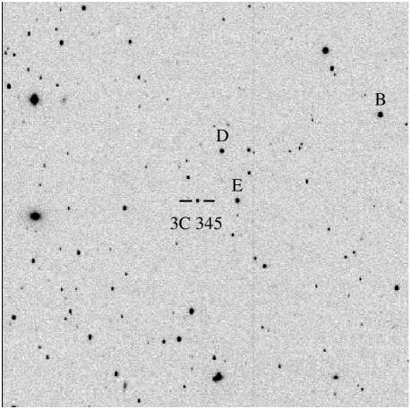
Figure 1: Finding chart of 3C 345, taken in the $i$ band on JD 245 4954. The blazar and three comparison stars are labelled. North is to the up and east, to the left.

2 Observations and Data Reductions

The monitoring was performed with a 60/90 cm Schmidt telescope at Xinglong station, National Astronomical Observatories of China. The telescope is equipped with a $4096\times 4096$ E2V CCD and 15 intermediate-band filters, which are used to do the Beijing-Arizona-Taiwan-Connecticut (BATC) survey (Zhou, 2005). The CCD has a pixel size of 12 $\micron$ and a spatial resolution of 1.3 $\arcsec{\rm pixel}^{-1}$. When used for blazar monitoring, only the central $512\times 512$ pixels are read out as a frame in order to reduce the readout time and to increase the sampling rate. Each such frame has a field of view of about $11^{\prime}\times 11^{\prime}$. The monitoring of 3C 345 was made in five intermediate bands, $c$, $e$, $i$, $m$ and $o$ ($e$, $i$ and $m$ bands in 2006 and $c$, $i$ and $o$ bands from 2007 to 2009). Their central wavelengths and bandwidths are listed in Table 1. The exposure times are generally 540, 300, 180, 300 and 480 s in the $c$, $e$, $i$, $m$ and $o$ bands, respectively, and may vary slightly depending on the weather and moon phase. An example frame in the $i$ band is shown in Fig. 1. 3C 345 and three reference stars are labelled. The reference stars are adopted from Smith et al. (1984). Their $c$, $e$, $i$, $m$ and $o$ magnitudes were obtained with observations on several photometric nights and are presented in Table 2. The data presented here cover the period from 2006 February 16 (JD 245 3783) to 2009 June 1 (JD 245 4984). More than 700 data points were collected on 53 nights.

Table 1: Central Wavelengths and Bandwidths of 5 BATC Filters

Filter	Central Wavelength	Bandwidth
	(Å)	(Å)
$c$	4206	289
$e$	4885	372
$i$	6685	514
$m$	8013	287
$o$	9173	248

The data reduction procedures include bias subtraction, flat-fielding, extraction of instrumental aperture magnitude, and flux calibration. The radii of the aperture and the sky annuli were adopted as 3, 7 and 10 pixels, respectively. The brightness of 3C 345 was calibrated relative to the average brightness of stars B and D. Star E acts as a check star. Its differential magnitude was also calculated relative to the average brightness of stars B and D, and was used to verify the accuracy of our observations.

Table 2: BATC $c$, $e$, $i$, $m$ and $o$ magnitudes of reference stars

Passband	B	D	E
$c$	14.933	16.286	16.951
$e$	14.782	15.885	16.183
$i$	14.118	15.069	14.728
$m$	13.974	14.886	14.332
$o$	13.852	14.706	14.115

Table 3: Statics on INOVs

JD	Band	Duration	$C$	Amplitude
		(hour)		(mag)
245 3783	$e$	1.62	2.750	0.104
245 3783	$i$	1.62	8.286	0.153
245 3783	$m$	1.62	5.545	0.154
245 3786	$i$	2.24	7.889	0.437
245 3786	$m$	2.25	5.048	0.252

3 Light Curves and Variation Amplitudes

Figure 2: Intra-night light curves of 3C 345 in the $e$, $i$ and $m$ bands on JD 245 3783 (large panels) and of the check stars (small panels).

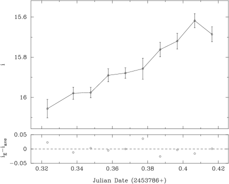
Figure 3: Intra-night light curves of 3C 345 in the $i$ and $m$ bands on JD 245 3786 (large panels) and of the check stars (small panels).

Among the 53 nights, 3C 345 shows INOVs on only 2 nights in 2006. The light curves on these 2 nights are displayed in Figs. 2 and 3. The large panels show the light curves of 3C 345, while the small panels give those of the check star. Following Jang & Miller (1997) and Romero, Cellone & Combi (1999), a variability parameter is defined as $C=\sigma_{\mathrm{T}}/\sigma$, where $\sigma_{\mathrm{T}}$ is the standard deviation of the magnitudes of the target blazar and $\sigma$ is that of the check star. The latter can be taken as the typical measurement error on a certain night. When $C\geqslant 2.576$, the object can be claimed to be variable at the 99% confidence level. The variability parameters were calculated for the five intra-night light curves, and the results are listed in Table 3. All five $C$ values are greater than 2.576, thus confirming the INOVs on these two nights. The variation amplitudes, as defined by Heidt & Wagner (1996), are also given in Table 3. The amplitude in the $e$ band is much less than those in the $i$ and $m$ bands on the same night.

Figure 4: Nightly-mean night curves of 3C 345 in five bands. For clarity, the $c$-, $e$-, $m$- and $o$-band magnitudes are shifted by 1.0, 1.0, $-$1.0 and $-$1.0 magnitudes, respectively.

3C 345 did not show INOV on the remaining 51 nights. Part of the reason may be the relatively short monitoring period on each single night in 2007–2009. Then its nightly average magnitudes were calculated and used for the following analyses. The nightly-averaged light curves are plotted in Fig. 4. Data in 5 different passbands are denoted with different symbols and are connected with different lines. One can see that there is at least one outburst from 2006 (JD 245 3800) to the first half of 2007 (JD 245 4250). Our recorded peak is at JD 245 3909, with $i=15.011\pm 0.011$, which corresponds to $R\sim 15.008$ with a simple interpolation between the fluxes in the $e$ and $i$ bands. However, we have very few observations during this period. So we cannot identify the exact time(s) and amplitude(s) (and/or number) of the outburst(s). From around JD 245 4200 to JD 245 4600, the object was monitored more or less constantly and declined gradually in brightness. After that, we again have few data and the object showed a tendency to recover till the end of our monitoring. The overall amplitude in the $i$ band (used in the whole monitoring period) is 2.640 mags. In 2006, where the source was monitored in the $e$, $i$ and $m$ bands, the variation amplitudes in the three bands are respectively 1.656, 1.829 and 1.731 mags. In 2007–2009 (or from JD 245 4192 to JD 245 4591), where the source was monitored in the $c$, $i$ and $o$ bands, the amplitudes are respectively 1.652, 1.964 and 1.947 mags. Then two conclusions can be drawn. Firstly, the amplitude in the $e$ or $c$ band is the smallest among those in the three bands ($e$, $i$ and $m$, or $c$, $i$ and $o$). This is similar to the case of the INOVs in this object mentioned above. Secondly, the $i$ band amplitude is greater than the corresponding $m$ or $o$ band amplitude.

Figure 5: Colour-magnitude diagrams of 3C 345 in 2006 (left panels) and in 2007–2009 (right panels). The upper four panels show RWB chromatism while the bottom two panels show BWB chromatism.

4 Colour Behaviour

The long-term colour behaviours of 3C 345 were studied by using the nightly-average magnitudes. For the 2006 data, the colour indices of $e-i$, $e-m$ and $i-m$ were calculated and plotted against $e$, $e$ and $i$, respectively, in the left panels of Fig. 5. For the 2007–2009 data, the colour indices of $c-i$, $c-o$ and $i-o$ were calculated and plotted against $c$, $c$ and $i$, respectively, in the right panels of Fig.  5. The $e-i$, $e-m$, $c-i$ and $c-o$ colours got redder when the source became brighter, whereas the $i-m$ and $i-o$ colours got bluer when the source became brighter. The correlation coefficients are respectively $-$0.958, $-$0.557, $-$0.794, $-$0.702, 0.707 and 0.307, and the chance probabilities are respectively $6.83\times 10^{-4}$, $1.94\times 10^{-1}$, $2.16\times 10^{-8}$, $1.06\times 10^{-5}$, $4.98\times 10^{-2}$ and $7.72\times 10^{-2}$. There are much fewer data points in the left panels than in the right ones, so the correlations in the left ones are weaker than those in the right ones, but the overall trends are the same.

For the two nights (JDs 245 3783 and 245 3786) showing INOVs, the colour-magnitude relation was also explored. Because there is no $e$-band observation on the latter night, we only studied the $i-m$ colour versus $i$ magnitude correlation. When calculating the $i-m$ colour, the $m$-band light curve on the two nights were linearly interpolated or extrapolated so as to get the $m$ magnitudes at exactly the same time when the $i$-band observations were made. The result is displayed in Fig. 6. The object tends to be BWB. The correlation coefficient is 0.809 and the chance probability is $8.37\times 10^{-5}$, indicating a strong BWB chromatism.

Figure 6: Colour-magnitude diagram of 3C 345 on JDs 245 3783 and 245 3786, the two nights showing INOVs. A strong BWB chromatism is visible.

Therefore, both RWB and BWB chromatisms were observed in the variability of 3C 345. This is quite different from the previous results on the spectral or colour behaviour of blazars, in which usually only one kind of colour behaviour is reported for one object. Or at most, an object, except for displaying either RWB or BWB chromatism in its middle- and short-term variability, may be achromatic for its long-term variability (e.g., Ghisellini et al., 1997; Villata et al., 2002; Raiteri et al., 2003) or during a certain episode of time (Wu et al., 2005; Poon, Fan & Fu, 2009). One exception is that Raiteri et al. (2003) have recognized both RWB and BWB trends in S5 0716+714, but at different times. Our study, however, revealed that the RWB and BWB chromatisms appeared in 3C 345 at the same time and/or in both the long-term variability and INOVs. This is the first report of such a phenomenon in the study of the colour behaviour of blazars.

5 Discussions

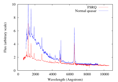
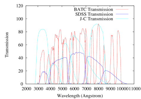
Figure 7: Composite quasar spectra and Transmission curves of three filter systems.

Several authors have studied the colour or spectral behaviour of 3C 345. They all found a RWB or steeper-when-brighter behaviour in the optical domain in this object (e.g., Kidger & Takalo, 1990; Schramm et al., 1993; Zhang et al., 2000; Mihov et al., 2008). However, there may be a cutoff magnitude ($R\approx 15.5$) in the colour-magnitude correlation, as noted by Mihov et al. (2008). When the object is brighter than that magnitude, its colour is much less dependent on the magnitude. This cutoff magnitude may also exist in the colour-magnitude diagrams in Mihov et al. (2008) and Zhang et al. (2000), but is not so obvious as in Schramm et al. (1993).

It has been suggested that a few components in the UV to blue band of the spectrum of 3C 345 may be responsible for the RWB or steeper-when-brighter behaviour (Kidger & Takalo, 1990; Schramm et al., 1993; Mihov et al., 2008). These components include the Mg ii emission line at 2798 Å and the blue bump (BB) from 1000 to 4000 Å in the rest frame of this object. The BB itself consists of a forest of the Fe ii emission lines, the Balmer continuum re-emission and the 10 000–40 000 K black body emission. Unlike the underlying non-thermal continuum (hereafter NTC), which is believed to come from the jet, these features come either from the accretion disc or from the BLR. Their variation properties should resemble those of the same emission features of normal quasars, i.e., they are variable but have smaller amplitudes and longer time-scales than the NTC variability of blazars (e.g. Ulrich, Maraschi & Urry, 2008; Benítez et al., 2010). When 3C 345 is in low state, these less variable emission features (hereafter LVEFs) dominate the fluxes and dilute the variability at short wavelengths. So the variation amplitudes at short wavelengths are smaller than those at long wavelengths, as manifested by Bregman et al. (1986) and this work (§3), leading naturally to a RWB behaviour when the measurements at short wavelengths ($U$, $B$, $V$, $c$ or $e$) are included in the colour calculation (Dai et al., 2011). When 3C 345 is in high state (brighter than the cutoff magnitude of $R=15.5$), the underlying NTC become strong and may match the LVEFs in strength. Then the object will show a stable colour, as illustrated in Schramm et al. (1993).

On the other hand, when the colour or spectral index is computed by using two measurements at long wavelengths where the LVEFs are not included in, we’ll get a BWB or flatter-when-brighter behaviour for 3C 345, as for its BWB behaviour in the $i-m$ and $i-o$ colours in this work and its flatter-when-brighter trend in the infrared regime in Bregman et al. (1986).

Similar colour behaviour has been observed for at least two more FSRQs. In 3C 454.3, the colour is RWB in faint state, reaches a ‘saturation’ at $R\approx 14$, and turns into BWB in bright state (Villata et al., 2006; Raiteri et al., 2008; Sasada et al., 2010a). These behaviours were also explained in terms of a thermal component, probably from the accretion disc, in the emission of 3C 454.3 (Raiteri et al., 2007, 2008; Sasada et al., 2010a). For PKS 1510-089, which has a pronounced BB in its spectrum (Singh et al., 1997; Kataoka et al., 2008), it exhibits a RWB trend except for its prominent flare, which can be explained by the strong contribution of thermal emission from the accretion disc (Sasada et al., 2010b).

Therefore, the Mg ii+BB emission can significantly change the colour behaviour of FSRQs. Except for the Mg ii line and the BB, there are some other strong emission features in the spectrum of FSRQs, such as the Ly$\alpha\,\lambda 1216$, C iv $\lambda 1549$, C iii]$\,\lambda 1909$, H$\beta\,\lambda 4861$+[O iii] $\lambda\lambda 4959,5007$+Fe ii and H$\alpha\,\lambda 6563$ lines. These features emanate from the BLR rather than from the jet, and are thus expected to be less variable than the underlying NTC. They may also significantly change the colour behaviour of FSRQs when one or more of them is included in the passbands that are used in the computation of the colour index, especially when the observations are made with an intermediate- or narrow-band filter system.

In order to assess how the emission lines change the measured fluxes in the passbands they reside, we then made a number of simulations by convolving the FSRQ spectrum with the transmission curves of several filter systems. The spectrum was shifted from 0 to 3 with a step of 0.01. Each spectrum was convolved with the transmission curves, so as to see the redshift effects on the measured fluxes.

We used a composite quasar spectrum to mimic the FSRQ spectrum in order to have a high signal-to-noise ratio and a large enough wavelength coverage. The FSRQ spectrum resembles the normal quasar spectrum in the content of the emission lines. However, their continua may differ much. The quasar spectrum usually has a strong BB, while the FSRQ spectrum has no or only weak BB due to the prominence of the strongly beamed jet emission (Jolley et al., 2009). We kept the emission features of the composite quasar spectrum but partly removed the BB from the continuum. The modified composite quasar spectrum was then used in the convolutions.

The composite quasar spectrum was adopted as a combination of the HST UV composite from 650 to 1150 Å (Zheng et al., 1997), the 2dF quasar composite from 1150 to 6930 Å (Croom et al., 2002) and a near-infrared composite from 6930 to 10600 Å (Glikman et al., 2006). We assigned a spectral index of 1.52 (Fossati et al., 1998) to the continuum from 1000 to 10600 Å and a spectral index of 2.6 for the continuum from 650 to 1000 Å, so as to add a weak BB into the continuum. The spectral index $\alpha$ is defined as $f_{\nu}\sim\nu^{-\alpha}$. This modified composite spectrum is plotted in the left panel of Fig. 7. For a comparison, the composite of the Large Bright Quasar Survey (LBQS, Francis et al., 1991) is also plotted, demonstrating the strong BB peaked at around 1300 Å. The right panel of Fig. 7 displays the transmission curves of the BATC (15 intermediate bands), SDSS (five broad bands, $u,g,r,i$ and $z$) and Johnson-Cousins (J-C, five broad band, $U,B,V,R$ and $I$) filter systems.

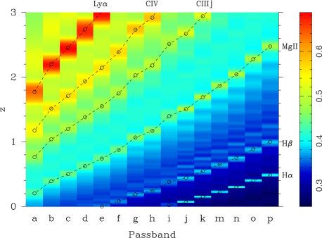
Figure 8: Observed fluxes of a FSRQ in the 15 intermediate BATC bands. The fluxes is plotted with colour in logarithm scale. The open circles denote the redshifts at which the emission lines move to the weighted centers of the passbands. The dashed lines are used to guide the ’movements’ of the emission lines with increasing redshift.

The convolutions were made at first between the composite spectrum and the BATC transmission curves. The resulting fluxes in the 15 intermediate bands were plotted in logarithm scale as colours in Fig. 8. The open circles label the redshifts at which the emission lines move to the weighted centers of the passbands. One can see from that figure that the strong emission lines move gradually from the short- to long-wavelength BATC passband with increasing redshift, as shown by the dashed lines. This figure demonstrates clearly that the strong emission lines can significantly enhance the measured fluxes in the passbands they are included in and that the enhancement changes with redshift. At the redshift close to 0.6, the fluxes of 3C 345 at the $c$, $d$ and $e$ bands are enhanced and dominated by the Mg ii line and the Fe ii lines on its both sides, especially during its faint state. On the other hand, the fluxes in the $i$, $m$ and $o$ bands are not enhanced by any strong emission lines and are dominated by the emission from the jet. So the $e-i$, $e-m$, $c-i$ and $c-o$ colours become RWB, while the $i-m$ and $i-o$ colours tend BWB, as mentioned at the beginning of this section.

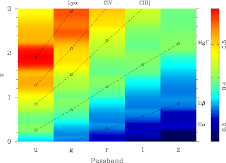
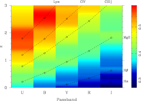
Figure 9: Same as Fig. 8 but for the SDSS and J-C filter systems.

Similar convolutions were made between the composite spectrum and the SDSS and J-C transmission curves. The results are plotted in Fig. 9. Due to the much broader passbands, which lower the flux dominance of the emission lines over the underlying NTC, and the partly overlapping of the adjacent passbands (see Fig. 7, right), the ’movements’ of the emission lines on the two maps are not so manifest as in Fig. 8, but the overall trends can still be seen. At some redshifts, more than one emission lines can be included in a same passband. For example, both the Ly$\alpha$ and C iv lines are included in the SDSS $g$ band and in the J-C $U$ band at a redshift of about 2.40 and 1.45, respectively, leading to a considerably enhanced fluxes at those two passbands. At the redshift close to 0.6, the $B$-band flux of 3C 345 is enhanced by the flux of Mg ii line, so its $B-V$ and $B-R$ colours show RWB trends when it is in low state. In the case of 3C 454.3, which is at a redshift of 0.859, its $V$-band flux is enhanced by the fluxes of the Mg ii line. So its $V-R$ and $V-K_{\mathrm{s}}$ colours show RWB trends when it is in low state.

The simulations clearly illustrate that the strong emssion lines can change the colour behaviours of FSRQs. Previous explanations for the RWB of FSRQs, either by the Mg ii+BB or by a thermal component, have in fact included the contributions from the strong emission lines of the Ly$\alpha$, C iv and C iii] lines. On the other hand, our simulations focus mainly on the emission lines, whose equivalent widths are usually less than 80 Å in the rest frame (Peterson, 1997). For the much broader ’emission’ feature, the BB, which can span from less than 1000 to about 4000 Å, a wavelength range much broader than the FWHM ($<1500$ Å) of a broad-band filter, the simulations cannot demonstrate whether it can change the colour behaviours. However, in the real cases, the broad (the BB) and narrow (the emission lines) LVEFs usually act simultaneously, especially in the $B$ and $V$ bands at low redshifts. This will lead to a RWB trend for the $B-R$, $V-R$, $V-J$ and $V-K_{\mathrm{s}}$ colours when the object is in faint state, as in the cases of 3C 345, 3C 454.3 and PKS 1510-089.

The simulations are not conclusive due to the different strengths of the LVEFs in different objects. In some objects, the LVEFs are intrinsically weak. Then the colour behaviour is expected to be BWB. This is in analogy to the case of BL Lac objects. Also, because of the broad passbands of the SDSS and J-C filters, there is a good chance for both the blue ($u$, $g$, $U$ and $B$) and the red passbands ($r$, $i$, $z$, $V$, $R$ and $I$) to include a strong emission feature. Then whether the object is RWB or BWB will depend on the interplay between the enhancements of the fluxes in the blue and red passbands. The most reliable way to study the spectral behaviour of FSQRs is to fit the continuum of their spectra. This will eliminate the impact of the LVEFs to the observed fluxes.

Most recently, Gu & Ai (2011) assembled a sample of 29 FSRQs in the SDSS Stripe 82 region. By fitting a power-law to the SDSS $ugriz$ photometric data, they found only one FSRQ showing RWB trend. This is quite different from previous results (Fan & Lin, 2000; Gu et al., 2006; Hu et al., 2006; Rani et al., 2010). The fitting of five photometric data points is somewhat similar to the fitting of the continuum, because the fluxes of the LVEFs cannot dominate in all five passbands, as can be seen in Fig. 9. So their results on the colour behaviour of FSRQs are more reasonable than the previous results.

6 Conclusions

We carried out a three-colour monitoring programme on the FSRQ, 3C 345 from 2006 February to 2009 June. There is at least one outburst during this period. The overall variation amplitude is 2.640 mags in the $i$ band. INOVs was observed on two nights. The BWB and RWB chromatisms were simultaneously detected in this object when using different pairs of passbands to compute the colours. The BWB chromatism is a shared property with the BL Lacs, while the RWB trend is likely due to two LVEFs, the Mg ii line and the blue bump, at short wavelengths.

We made numerical simulations by convolving a composite quasar spectrum with three filter systems. The results indicate that some other strong but less variable emission lines, such as the Ly$\alpha$, C iv, C iii], H$\beta$+[O iii] and H$\alpha$ lines, in the spectrum of FSRQs may also significantly enhance the measured fluxes of the passbands they are included in, and hence change the colour behaviour of the object.

The emission of BL Lac objects is dominated by the beamed NTC from the relativistic jet. However, the emission from FSRQs should be a combination of the NTC from the jet, the thermal emission from the accretion disc and the line emission from the BLR. The two latter components are collectively name as LVEFs in this paper. The beamed NTC from the jet tends to show BWB chromatism, no matter in BL Lacs or FSRQs. The LVEFs in FSRQs can significantly change their colour behaviours, especially when they are in faint state.

The factors that govern the colour behaviour of FSRQs can be summarized as follows.

1. The relative strengths of the LVEFs and the NTC. The relative strengths of the two components can be different for different objects, and are related to the brightness states of the objects. Strong LVEFs but weak NTC will result in RWB trend, while weak LVEFs and strong NTC will lead to in BWB chromatism.

2. The redshift. The redshift decides the wavelengths of the observed LVEFs.

3. The passbands used for colour calculation. Different passbands will include different LVEFs.

7 Acknowledgements

The authors thank the anonymous referee for insightful suggestions and comments. We thank M. Gu for useful discussions. This work has been supported by Chinese National Natural Science Foundation grants 10873016, and 11073032, and by the National Basic Research Programme of China (973 Programme) No. 2007CB815403.

References

- Aller et al. (1985) Aller H.D., Aller M.F., Latimer G.E., Hodge P.E., 1985, ApJS, 59, 513
- Babadzhanyants et al. (1985) Babadzhanyants M.K., Belokon E.T., Denisenko N.S., Semënova E.V., 1985, Soviet Astronomy, 29, 394
- Belokon & Babadzhanyants (1999) Belokon E.T., Babadzhanyants M.K., 1999, Astronomy Letters, 25, 893
- Benítez et al. (2010) Benítez E., Chavushyan V.H., Raiteri C.M., Villata M., Dultzin D., Martínez O., Pérez-Camargo B., Torrealba J., 2010, ASPC, 427, 291
- Böttcher (2007) Böttcher M., 2007, ApS&S, 309, 95
- Böttcher et al. (2007) Böttcher M. et al., 2007, ApJ, 670, 968
- Böttcher et al. (2009) Böttcher M. et al., 2009, ApJ, 694, 174
- Bregman et al. (1986) Bregman J.N. et al., 1986, ApJ, 301, 708
- Burbidge (1965) Burbidge E.M., 1965, ApJ, 142, 1674
- Caproni & Abraham (2004) Caproni A., Abraham Z., 2004, ApJ, 602, 625
- Croom et al. (2002) Croom S.M. et al., 2002, MNRAS, 337, 275
- Dai et al. (2011) Dai Y., Wu J., Zhu Z., Zhou X., Ma J., 2011, AJ, 141, 65
- Fan & Lin (2000) Fan J., Lin R., 2000, ApJ, 537, 101
- Fossati et al. (1998) Fossati G., Maraschi L., Celotti A., Comastri A., Ghisellini G., 1998, MNRAS, 299, 433
- Francis et al. (1991) Francis P.J. et al., 1991, ApJ, 373, 465
- Ghisellini et al. (1997) Ghisellini G. et al., 1997, A&A, 327, 61
- Glikman et al. ( 2006) Glikman E.. Helfand D.J., White R.L., 2006, ApJ, 640, 579
- Gu et al. (2006) Gu M.F., Lee C.-U., Pak S., Yim H.S., Fletcher A.B. 2006, A&A, 450, 39
- Gu & Ai (2011) Gu M.F., Ai Y.L., 2011, A&A, 528, 95
- Heidt & Wagner (1996) Heidt J., Wagner S.J., 1996, A&A, 305, 42
- Hu et al. (2006) Hu S., Zhao G., Guo H.Y., Zhang X., Zheng Y.G., 2006, MNRAS, 371, 1243
- Jang & Miller (1997) Jang M., Miller H.R., 1997, AJ, 114, 565
- Jolley et al. (2009) Jolley E.J.D., Kuncic Z., Bicknell G.V., Wagner S., 2009, MNRAS, 400, 1521
- Kataoka et al. (2008) Kataoka J. et al., 2008, ApJ, 672, 787
- Kinman et al. (1968) Kinman T.D., Lamla E., Ciurla T., Harlan E., Wirtanen C.A., 1968, ApJ, 152, 357
- Kidger & Beckman (1986) Kidger M.R., Beckman J.E., 1986, A&A, 154, 288
- Kidger (1989) Kidger M.R., 1989, A&A, 226, 9
- Kidger & de Diego (1990) Kidger M.R., de Diego J.A., 1990, A&A, 227, L25
- Kidger & Takalo (1990) Kidger M.R., Takalo L., 1990, A&A, 239, L9
- Kollgaard et al. (1989) Kollgaard R.I., Wardle J.F.C., Roberts D.H., 1989, AJ, 97, 1550
- Lobanov & Roland (2005) Lobanov A.P., Roland J., 2005, A&A, 431, 831
- Marziani et al. (1996) Marziani P., Sulentic J.W., Dultzin-Hacyan D., Calvani M., Moles M., 1996, ApJS, 104, 37
- McGimsey et al. (1975) McGimsey B.Q., Smith A.G., Scott R.L., Leacock R.J., Edwards P.L., Hackney R.L., Hackney K.R., 1975, AJ, 80, 895
- Mihov et al. (2008) Mihov B., Bachev R., Slavcheva-Mihova L., Strigachev A., Semkov E., Petrov G., 2008, AN, 329, 77
- Perley et al. ( 1982) Perley R.A., Fomalont E.B., Johnston K.J., 1982, ApJ, 255, L93
- Peterson (1997) Peterson B.M., An Introduction to Active Galactic Nuclei, Cambridge Univ. Press, Cambridge, p16
- Poon et al. (2009) Poon H., Fan J.H., Fu J.N., 2009, ApJS, 185, 511
- Raiteri et al. (2003) Raiteri C.M. et al., 2003, A&A, 402, 151
- Raiteri et al. (2007) Raiteri C.M. et al., 2007, A&A, 473, 819
- Raiteri et al. (2008) Raiteri C.M. et al., 2008, A&A, 491, 755
- Ramírez et al. (2004) Ramírez A., de Diego J.A., Dultzin-Hacyan D., González-Pérez J.N., 2004, A&A, 421, 83
- Rani et al. (2010) Rani B. et al., 2010, MNRAS, 404, 1992
- Romero et al. ( 1999) Romero G.E., Cellone S.A., Combi J.A., 1999, A&A, 135, 477
- Sasada et al. (2010a) Sasada M. et al., 2010, PASJ, 62, 645
- Sasada et al. (2010b) Sasada M. et al., 2010, PASJ, 63, 489
- Schramm et al. (1993) Schramm K.-J. et al., 1993, A&A, 278, 391
- Singh et al. ( 1997) Singh K.P., Shrader C.R., George I.M., 1997, ApJ, 491, 515
- Smith et al. (1984) Smith P.S., Balonek T.J., Heckert P.A., Elston R., Schmidt G.D., 1985, AJ, 90, 1184
- Smith et al. (1986) Smith P.S., Balonek T.J., Heckert P.A., Elston R., 1986, ApJ, 305, 484
- Ulrich et al. ( 2008) Ulrich M.-H., Maraschi L., Urry C.M., 1997, ARA&A, 35, 445
- Vagnetti et al. (2003) Vagnetti F., Trevese D., Nesci R., 2003, ApJ, 590, 123
- Villata et al. (2002) Villata M. et al., 2002, A&A, 390, 407
- Villata et al. (2006) Villata M. et al., 2006, A&A, 453, 817
- Webb et al. (1988) Webb J.R., Smith A.G., Leacock R.J., Fitzgibbons G.L., Gombola P.P., Shepherd D.W., 1988, AJ, 95, 374
- Webb et al. (1994) Webb J.R. et al., 1994, ApJ, 422, 570
- Wu et al. (2005) Wu J., Peng B., Zhou X., Ma J., Jiang Z., Chen J., 2005, AJ, 129, 1818
- Wu et al. (2007) Wu J., Zhou X., Ma J., Wu Z., Jiang Z., Chen J., 2007, AJ, 133, 1599
- Zhang et al. (2000) Zhang X., Xie G.Z., Bai J.M., Zhao G., 2000, A&AS, 271, 1
- Zheng et al. (1997) Zheng W., Kriss G.A., Telfer R.C., Grimes J.P., Davidsen A.F., 1997, ApJ, 475, 469
- Zhou (2005) Zhou X., 2005, JKAS, 38, 203