Turing degrees of multidimensional SFTs

Abstract

In this paper we are interested in computability aspects of subshifts and in particular Turing degrees of 2-dimensional SFTs (i.e. tilings). To be more precise, we prove that given any $\Pi^{0}_{1}$ class $P$ of $\left\{0,1\right\}^{\mathbb{N}}$ there is a SFT $X$ such that $P\times\mathbb{Z}^{2}$ is recursively homeomorphic to $X\setminus U$ where $U$ is a computable set of points. As a consequence, if $P$ contains a computable member, $P$ and $X$ have the exact same set of Turing degrees. On the other hand, we prove that if $X$ contains only non-computable members, some of its members always have different but comparable degrees. This gives a fairly complete study of Turing degrees of SFTs.

Wang tiles have been introduced by Wang [Wang(1961)] to study fragments of first order logic. Independently, subshifts of finite type (SFTs) were introduced to study dynamical systems. From a computational and dynamical perspective, SFTs and Wang tiles are equivalent, and most recursive-flavoured results about SFTs were proved in a Wang tile setting.

Knowing whether a tileset can tile the plane with a given tile at the origin (also known as the origin constrained domino problem) was proved undecidable by Wang [Wang(1963)]. Knowing whether a tileset can tile the plane in the general case was proved undecidable by Berger [Berger(1964), Berger(1966)].

Understanding how complex, in the sense of recursion theory, the points of an SFT can be is a question that was first studied by Myers [Myers(1974)] in 1974. Building on the work of Hanf [Hanf(1974)], he gave a tileset with no computable tilings. Durand/Levin/Shen [Durand et al.(2008)Durand, Levin, and Shen] showed, 40 years later, how to build a tileset for which all tilings have high Kolmogorov complexity.

A $\Pi^{0}_{1}$ class (of sets) is an effectively closed subset of $\left\{0,1\right\}^{\mathbb{N}}$, or equivalently the set of oracles on which a given Turing machine does not halt. $\Pi^{0}_{1}$ classes occur naturally in various areas in computer science and recursive mathematics, see e.g. [Cenzer and Remmel(1998), Simpson(2011a)] and the upcoming book [Cenzer and Remmel(2011)]. It is easy to see that any SFT is a $\Pi^{0}_{1}$ class (up to a computable coding of $\Sigma^{\mathbb{Z}^{2}}$ into $\left\{0,1\right\}^{\mathbb{N}}$). This has various consequences. As an example, every non-empty SFT contains a point which is not Turing-hard (see Durand/Levin/Shen [Durand et al.(2008)Durand, Levin, and Shen] for a self-contained proof). The main question is how different SFTs are from $\Pi^{0}_{1}$ classes. In the one-dimensional case, some answers to these questions were given by Cenzer/Dashti/King/Tosca/Wyman [Dashti(2008), Cenzer et al.(2008)Cenzer, Dashti, and King, Cenzer et al.(2012)Cenzer, Dashti, Toska, and Wyman].

The main result in this direction was obtained by Simpson [Simpson(2011b)], building on the work of Hanf and Myers: for every $\Pi^{0}_{1}$ class $S$, there exists a SFT with the same Medvedev degree as $S$. The Medvedev degree roughly relates to the “easiest” Turing degree of $S$. What we are interested in is a stronger result: can we find for every $\Pi^{0}_{1}$ class $S$ a SFT which has the same Turing degrees? We prove in this article that this is true if $S$ contains a computable point but not always when this is not the case. More exactly we build (Theorem 4.1) for every $\Pi^{0}_{1}$ class $S$ a SFT for which the set of Turing degrees is exactly the same as for $S$ with the additional Turing degree of computable points. We also show that SFTs that do not contain any computable point always have points with different but comparable degrees (Corollary 5.11), a property that is not true for all $\Pi^{0}_{1}$ classes. In particular there exist $\Pi^{0}_{1}$ classes that do not have any points with comparable degrees.

As a consequence, as every countable $\Pi^{0}_{1}$ class contains a computable point, the question is solved for countable sets: the sets of Turing degrees of countable $\Pi^{0}_{1}$ classes are the same as the sets of Turing degrees of countable sets of tilings. In particular, there exist countable sets of tilings with some non-computable points. This can be thought as a two-dimensional version of Corollary 4.7 in [Cenzer et al.(2012)Cenzer, Dashti, Toska, and Wyman].

This paper is organized as follows. After some preliminary definitions, we start with a quick proof of a generalization of Hanf, already implicit in Simpson [Simpson(2011b)]. We then build a very specific tileset, which forms a grid-like structure while having only countably many tilings, all of them computable. This tileset will then serve as the main ingredient to prove the result on the case of classes with a computable point in section 4. In section 5 we finally show the result on classes without computable points.

1 Preliminaries

1.1 SFTs and tilings

We give here some standard definitions and facts about multidimensional subshifts, one may consult Lind [Lind(2004)] for more details. Let $\Sigma$ be a finite alphabet, the $d$-dimensional full shift on $\Sigma$ is the set $\Sigma^{\mathbb{Z}^{d}}=\left\{c=(c_{x})_{x\in\mathbb{Z}^{d}}\middle|\forall x\in\mathbb{Z}^{d},c_{x}\in\Sigma\right\}$. For $v\in\mathbb{Z}^{d}$, the shift functions $\sigma_{v}:\Sigma^{\mathbb{Z}^{d}}\to\Sigma^{\mathbb{Z}^{d}}$, are defined locally by $\sigma_{v}(c_{x})=c_{x+v}$. The full shift equipped with the distance $d(x,y)=2^{-\min\left\{\left\|v\right\|\middle|v\in\mathbb{Z}^{d},x_{v}\neq y_{v}\right\}}$ is a compact, perfect, metric space on which the shift functions act as homeomorphisms. An element of $\Sigma^{\mathbb{Z}^{d}}$ is called a configuration.

Every closed shift-invariant (invariant by application of any $\sigma_{v}$) subset $X$ of $\Sigma^{\mathbb{Z}^{d}}$ is called a subshift. An element of a subshift is called a point of this subshift.

Alternatively, subshifts can be defined with the help of forbidden patterns. A pattern is a function $p:P\to\Sigma$, where $P$ is a finite subset of $\mathbb{Z}^{d}$. Let $\mathcal{F}$ be a collection of forbidden patterns, the subset $X_{F}$ of $\Sigma^{\mathbb{Z}^{d}}$ containing only configurations having nowhere a pattern of $F$. More formally, $X_{\mathcal{F}}$ is defined by

$$X_{\mathcal{F}}=\left\{x\in\Sigma^{\mathbb{Z}^{d}}\middle|\forall z\in\mathbb{Z}^{d},\forall p\in\mathcal{F},x_{z+P}\neq p\right\}\textrm{.}$$

In particular, a subshift is said to be a subshift of finite type (SFT) when the collection of forbidden patterns is finite. Usually, the patterns used are blocks or $n$-blocks, that is they are defined over a finite subset $P$ of $\mathbb{Z}^{d}$ of the form ${\llbracket 0,n-1\rrbracket}^{d}$.

Given a subshift $X$, a block or pattern $p$ is said to be extensible if there exists $x\in X$ in which $p$ appears, $p$ is also said to be extensible to $x$.

In the rest of the paper, we will use the notation $\Sigma_{X}$ for the alphabet of the subshift $X$.

A subshift $X\subseteq\Sigma_{X}^{\mathbb{Z}^{2}}$ is a sofic shift if and only if there exists a SFT $Y\subseteq\Sigma_{Y}^{\mathbb{Z}^{2}}$ and a map $f:\Sigma_{Y}\rightarrow\Sigma_{X}$ such that for any point $x\in X$, there exists a point $y\in Y$ such that for all $z\in\mathbb{Z}^{d},x_{z}=f(y_{z})$.

Wang tiles are unit squares with colored edges which may not be flipped or rotated. A tileset $T$ is a finite set of Wang tiles. A coloring of the plane is a mapping $c:\mathbb{Z}^{2}\rightarrow T$ assigning a Wang tile to each point of the plane. If all adjacent tiles of a coloring of the plane have matching edges, it is called a tiling.

In particular, the set of tilings of a Wang tileset is a SFT on the alphabet formed by the tiles. Conversely, any SFT is isomorphic to a Wang tileset. From a recursivity point of view, one can say that SFTs and Wang tilesets are equivalent. In this paper, we will be using both indiscriminately. In particular, we denote by $X_{T}$ the SFT associated to a set of tiles $T$.

We say a SFT (tileset) is origin constrained when the letter (tile) at position $(0,0)$ is forced, that is to say, we only look at the valid tilings having a given letter (tile) $t$ at the origin.

More information on SFTs may be found in Lind and Marcus’ book [Lind and Marcus(1995)].

The notion of Cantor-Bendixson derivative is defined on set of configurations. This notion was introduced for tilings by Ballier/Durand/Jeandel [Ballier et al.(2008)Ballier, Durand, and Jeandel]. A configuration $c$ is said to be isolated in a set of configurations $C$ if there exists a pattern $p$ such that $c$ is the only configuration of $C$ containing $p$. The Cantor-Bendixson derivative of $C$ is denoted by $D(C)$ and consists of all configurations of $C$ except the isolated ones. We define $C^{(\lambda)}$ inductively for any ordinal $\lambda$:

• $C^{(0)}=S$

• $C^{(\lambda+1)}=D\left(C^{\left(\lambda\right)})\right)$

• $C^{(\lambda)}=\bigcap_{\gamma<\lambda}C^{(\gamma)}$ when $\lambda$ is a limit ordinal.

The Cantor-Bendixson rank of $C$, denoted by $CB(C)$, is defined as the first ordinal $\lambda$ such that $C^{(\lambda)}=C^{(\lambda+1)}$. If $C$ is countable, then $C^{CB(C)}$ is empty. An element $x$ is of rank $\lambda$ in $C$ if $\lambda$ is the least ordinal such that $x\not\in C^{(\lambda)}$.

A configuration $x$ is periodic, if there exists $n\in\mathbb{N}^{*}$ such that $\sigma_{ne_{i}}(x)=x$, for any $i\in\{1,\dots,d\}$, where the $e_{i}$’s form the standard basis. A vector of periodicity of a configuration is a vector $v\in\mathbb{Z}^{d}\setminus\{(0,\dots,0)\}$ such that $\sigma_{v}(x)=x$. A configuration $x$ is quasiperiodic (see Durand [Durand(1999)] for instance) if for any pattern $p$ appearing in $x$, there exists $N$ such that this pattern appears in all $N^{d}$ cubes in $x$. In particular, a periodic point is quasiperiodic. A configuration is strictly quasiperiodic if it is quasiperiodic and not periodic. A subshift is minimal if it is non-empty and contains no proper non-empty subshift. Equivalently, all its points have the same patterns. In this case, it contains only quasiperiodic points. It is known that every subshift contains a minimal subshift, see e.g. Durand [Durand(1999)].

1.2 Computability background

A $\Pi^{0}_{1}$ class $P\subseteq\left\{0,1\right\}^{\mathbb{N}}$ is a class of infinite sequences on $\{0,1\}$ for which there exists a Turing machine that given $x\in\left\{0,1\right\}^{\mathbb{N}}$ as an oracle halts if and only if $x\not\in P$. Equivalently, a class $S\subseteq\left\{0,1\right\}^{\mathbb{N}}$ is $\Pi^{0}_{1}$ if there exists a computable set $L$ so that $x\in S$ if and only if no prefix of $x$ is in $L$. An element of a $\Pi^{0}_{1}$ class is called a member of this class.

We say that two sets $S,S^{\prime}$ are recursively homeomorphic if there exists a bijective computable function $f:S\rightarrow S^{\prime}$. That is to say there are two Turing machines $M$ (resp. $M^{\prime}$) such that given a member of $S$ (resp. $S^{\prime}$) computes a member of $S^{\prime}$ (resp. $S$). Furthermore, for any $s\in S,s^{\prime}\in S^{\prime}$ such that $s^{\prime}$ is computed by $M$ from $s$, $M^{\prime}$ computes $s$ from $s^{\prime}$.

The Cantor-Bendixson rank of $S$, is well defined similarly as for subshifts.

See Cenzer/Remmel [Cenzer and Remmel(1998)] for $\Pi^{0}_{1}$ classes and Kechris [Kechris(1995)] for Cantor-Bendixson rank and derivative.

For $x,y\in\left\{0,1\right\}^{\mathbb{N}}$ we say that $x$ is Turing-reducible to $y$ if $y$ is computable by a Turing machine using $x$ as an oracle and we write $y\leq_{T}x$. If $x\leq_{T}y$ and $y\leq_{T}x$, we say that $x$ and $y$ are Turing-equivalent and we write $x\equiv_{T}y$. The Turing degree of $x\in\left\{0,1\right\}^{\mathbb{N}}$, denoted by $\deg_{T}x$, is its equivalence class under the relation $\equiv_{T}$.

1.3 Subshifts and $\Pi^{0}_{1}$ classes

As is clear from the definitions, SFTs in any dimension are $\Pi^{0}_{1}$ classes. More generally, effective subshifts, see e.g. Cenzer/Dashti/King [Cenzer et al.(2008)Cenzer, Dashti, and King]), that is subshifts defined by a computable (or equivalently, in this case, by a computably enumerable) set of forbidden patterns are $\Pi^{0}_{1}$ classes. As such, they enjoy similar properties. In particular, there exist many “basis theorems”, i.e.theorems that assert that any $\Pi^{0}_{1}$ (non-empty) class has a member with some specific property.

As an example, every countable $\Pi^{0}_{1}$ class has a computable member, see e.g. Cenzer/Remmel [Cenzer and Remmel(2011)]. For subshifts, we can say a bit more: every countable subshift has a periodic (hence computable) member.

Some basis theorems for $\Pi^{0}_{1}$ classes can be easily reproven in the context of subshifts: The proof that every $\Pi^{0}_{1}$ class has a point of low degree (the formal definition is not important here, but it can be interpreted as “nearly computable”) [Jockusch and Soare(1972b)] was reproven for subshifts (actually tilings) in Durand/Levin/Shen [Durand et al.(2008)Durand, Levin, and Shen].

2 $\Pi^{0}_{1}$ classes and origin constrained tilings

A straighforward corollary of Hanf [Hanf(1974)] is that every $\Pi^{0}_{1}$ class is recursively homeomorphic to an origin constrained SFTs and conversely. This is stated explicitly in Simpson [Simpson(2011b)].

Figure 1: A set of Wang tiles, encoding computation of a Turing machine: the states are in the circles and the tape is in the rectangles. The bottom right tile starts computations. A tiling containing this tile contains the space-time diagram of some run of the Turing machine.

Theorem 2.1.

Given any $\Pi^{0}_{1}$ class $P\subseteq\left\{0,1\right\}^{\mathbb{N}}$, there exists a SFT $X$ and a letter $t\in\Sigma_{X}$ such that each origin constrained point corresponds to a member of $P$.

Proof.

Let $P$ be a $\Pi^{0}_{1}$ class, and $M$ the Turing machine that proves it, that is $M$ given $x\in\left\{0,1\right\}^{\mathbb{N}}$ as an oracle halts if and only if $x\not\in P$.

We use the classic encoding of Turing machines as Wang tiles, see fig. 1. We modify all tiles containing a symbol from the tape, to allow them to contain a second symbol. This symbol is copied vertically. All these second symbols represent the oracle.

Then the SFT constrained by the tile starting the computation contains exactly the runs of the Turing machine with members of $P$ on the oracle tape. ∎

Corollary 2.2.

Any $\Pi^{0}_{1}$ class $P$ of $\left\{0,1\right\}^{\mathbb{N}}$ is recursively homeomorphic to an origin constrained SFT.

3 Producing a sparse grid

The main problem in the previous construction is that points which do not have the given letter at the origin can be very wild: they may correspond to configurations with no computation (no head of the Turing Machine) or computations starting from an arbitrary (not initial) configuration. A way to solve this problem is described in Myers’ paper [Myers(1974)] but is unsuitable for our purposes (It was however used by Simpson to obtain a weaker result on Medvedev degrees, see [Simpson(2011b)]).

Figure 2: The tiling in which the Turing machines will be encoded.

Our idea is as follows: we build a SFT which will contain, among other points, the sparse grid of Figure 2c. The interest being that all other points will have at most one intersection of two black lines. This means that if we put computation cells of a given Turing machine in the intersection points, every point which is not of the form of Figure 2c will contain at most one cell of the Turing machine, and thus will contain no computation.

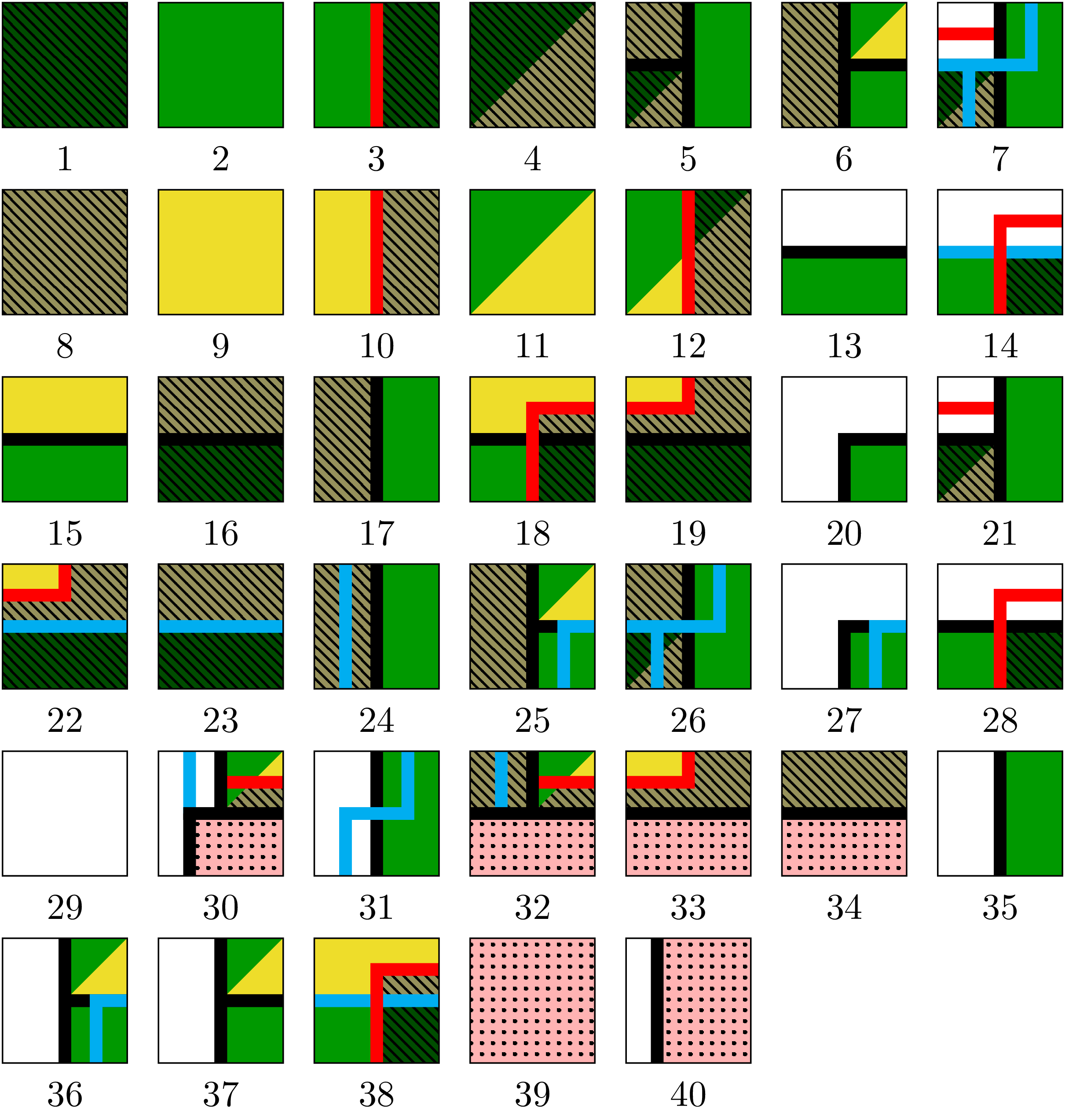
Figure 3: Our set of Wang tiles $T$.

To do this construction, we will first draw increasingly big and distant columns as in Figure 2a and then superimpose the same construction for rows as in Figure 2b, thus obtaining the grid of Figure 2c.

It is then fairly straightforward to see how we can encode a Turing machine inside a configuration having the skeleton of Figure 2c by looking at it diagonally: time increases going to the north-east and the tape is written on the north-west/south-east diagonals.

Our set of tiles $T$ of Figure 3 gives the skeleton of Figure 2a when forgetting everything but the black vertical borders. We will prove in this section that it is countable. We set here the vocabulary:

• tile 30 is the corner tile

• tile 20 and 27 are the top tiles

• tiles 30, 32, 33, 34 are the bottom tiles

• a vertical line is formed of a vertical succession of tiles containing a vertical black line (tiles 5, 6, 7, 17, 21, 24, 25, 26, 31, 35, 36, 37), which may be ended by bottom and/or top tiles.

• a horizontal line is formed of a horizontal succession of tiles containing a horizontal black line (tiles 13, 14, 15, 16, 18, 19, 22, 23, 28, 32, 33, 34, 38), and may be ended by tiles 5,6,7,25,26,36,37, thus forcing a vertical line at this end,

• a diagonal is a diagonal succession (positions (i,j),(i+1,j+1),…) of tiles among 4,12,11,

• a square is a $\llbracket 0,k\rrbracket^{2}$ valid tiling such that $\{0\}\times\llbracket 1,k-1\rrbracket$ and $\{k\}\times\llbracket 1,k-1\rrbracket$ are vertical lines, and $\llbracket 1,k-1\rrbracket\times\{0\}$ and $\llbracket 1,k-1\rrbracket\times\{k\}$ are horizontal lines. Remark that the color on the right of the first column and on the left of the last one force the existence of a counting signal inbetween and of a diagonal tile on each of the $(i,i)$ positions for $0<i<k$.

• the increase signal is formed by a path of tiles among 7, 14, 22, 23, 24, 25, 26, 27, 30, 31, 36, 38, such that the blue signal is connected, this signal will force the squares to increase in size by exactly one in each column.

• the counting signal is formed by a path of tiles among 3 ,7, 10, 12, 14, 19, 22, 32, 33, 38, such that the counting signal is connected. It may be ended only by tiles 30,32 and 7,21. This signal will force the number of squares in each column to be at most the size of these squares.

Note that whenever the corner tile appears in a point, it is necessarily a shifted copy of the point on Figure 4: the corner tile forces the tiles on its right to be bottom tiles and the first above to be tile 33, then on top of it must be tile 31 and then tile 27. This forces the existence of the first square, i.e.the first column. Then the increase signal forces the second column to start with a square of size increased by one, and thus to have exactly one more square (increase signal), and so on.

Lemma 3.1.

The SFT $X_{T}$ admits at most one point, up to translation, with two or more vertical lines. This point is drawn on Figure 4.

Proof.

The idea of the construction is to force that whenever there are two vertical lines, then the point is a shifted copy of the one in Figure 4.

Suppose that we have a tiling in which two vertical lines appear. They may be ended on their bottom only by a bottom tile 30 or 32, but when a bottom tile appears, it forces all tiles to its right to be bottom tiles. Because the color on each side of the vertical lines is not the same they necessarily are connected by horizontal lines, which must form squares due to the diagonal. Suppose the two vertical lines are at distance $k$, then there are exactly $k$ squares between them vertically, because of the counting signal: it must appear in each square, and is shifted to the right every time it crosses a horizontal line, it may be ended in each column only by tiles 32 (or 30 if it is the leftmost column) in the bottommost square and by 21 (resp. 7) in the topmost.

The bottommost square must have an increase signal as its top horizontal line, since the lower left corner 32 (or 30 in case it is the leftmost square) forces the left side to be formed of a succession of tiles 24 ended by tile 26 (resp. only one tile 31), then the top left corner is necessarily a tile 25 (resp. 27). This forces the size of the squares on its left to be $k-1$ and on its right to be $k+1$.

If we focus only on the bottommost squares, they are of decreasing size when going left, the last one is of size 1, and necessarily has the corner tile as its lower left corner. ∎

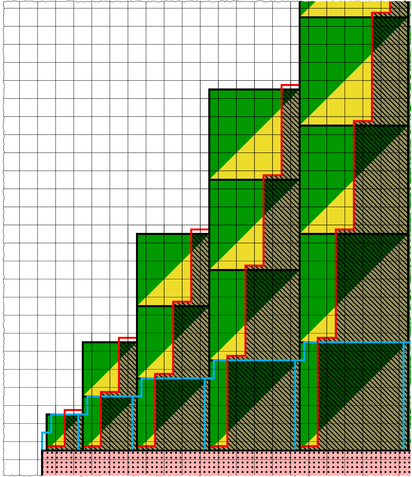
Figure 4: Tiling $\alpha$: the unique valid tiling of $T$ in which there are 2 or more vertical lines. This tiling has Cantor-Bendixson rank 1.

Lemma 3.2.

$X_{T}$ is countable.

Proof.

Lemma 3.1 states that there is one point, up to shift, that has two or more vertical lines. This means that the other points have at most one such line.

• If a point has exactly one vertical line, then it can have at most two horizontal lines: one on the left of the vertical one and one on the right. Otherwise a square would appear and the configuration would be $\alpha$. A counting signal may then appear on the left or the right of the vertical line arbitrarily far from it. There is a countable number of such points.

• If a point has no vertical line, then it has at most one horizontal line. A counting signal can then appear only once. There is a finite number of such points, up to shift.

There is a countable number of points that can be obtained with the tileset $T$. All types of obtainable points are shown in Figures 4 and 5.

∎

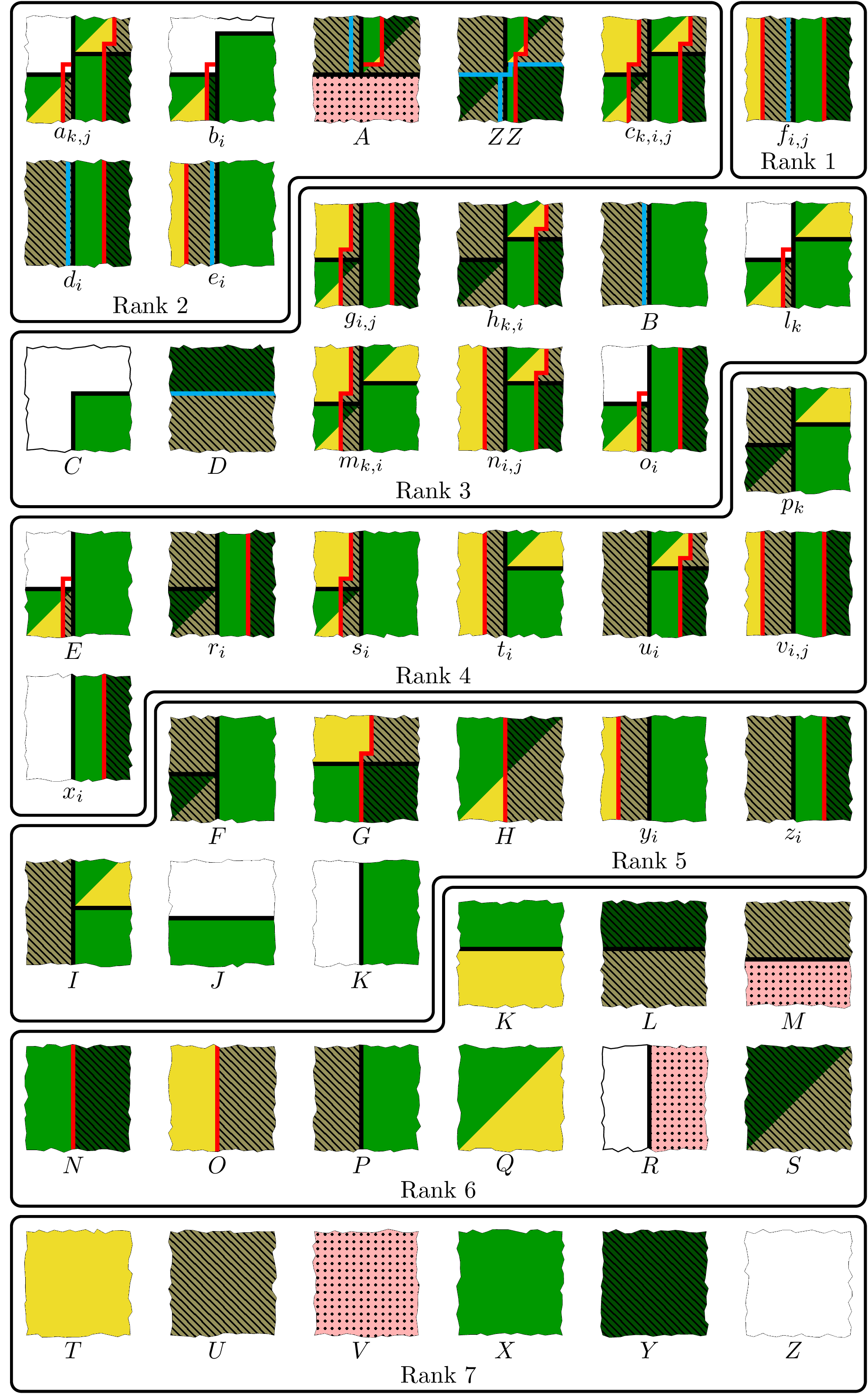
Figure 5: The configurations of $X_{T}\setminus\{\alpha\}$: the $A-ZZ$ configurations are unique (up to shift), and the configurations with subscripts $i,j\in\mathbb{N},k\in\mathbb{Z}^{2}$ represent the fact that distances between some of the lines (red, horizontal, vertical) can vary. The configurations are classified according to their Cantor-Bendixson rank. Note that configuration $ZZ$ cannot have a counting signal on its left, because it would force another vertical line.

By taking our tileset $T=\{1,\dots,40\}$ and mirroring all the tiles along the south-west/north-east diagonal, we obtain a tileset $T^{\prime}=\{1^{\prime},\dots,40^{\prime}\}$ with the exact same properties, except it enforces the skeleton of Figure 2b. Remember that whenever the corner tile appeared in a point, then necessarily this point was a shifted of $\alpha$. Analogously, the corner tile of $T^{\prime}$ appearing in a point means that this point is a shifted of $\alpha^{\prime}$. We hence construct a third tileset $\tau=\left(T\setminus\left\{30\right\}\times T^{\prime}\setminus\left\{30^{\prime}\right\}\right)\cup\left\{(30,30^{\prime})\right\}$ which is the superimposition of $T$ and $T^{\prime}$ with the restriction that tiles $30$ and $30^{\prime}$ are necessarily superimposed to each other. The corner tile $(30,30^{\prime})$ of $\tau$ has the property that whenever it appears, the tiling is the superimposition of the skeletons of Figures 2a and 2b with the corner tiles at the same place: there is only one such tiling up to shift, we call it $\beta$.

The skeleton of Figure 2c is obtained from $\beta$ if we forget about the parts of the lines of the $T$ layer (resp. $T^{\prime}$) that are superimposed to white tiles, 29’ (resp. 29), of $T^{\prime}$ (resp. $T$).

As a consequence of Lemma 3.2, $X_{\tau}$ is also countable. And as a consequence of Lemma 3.1, the only points in $x_{\tau}$ in which computation can be embedded are the shifts of $\beta$. The shape of $\beta$ is the one of Figure 2c, the coordinates of the points of the grid are the following (supposing tile $(30,30^{\prime})$ is at the center of the grid):

$$\left\{(f(n),f(m))\mid f(m)/4\leq f(n)\leq 4f(m)\right\}$$

$$\left\{(f(n),f(m))\mid m/2\leq n\leq 2m\right\}$$

where $f(n)=(n+1)(n+2)/2-1$.

Lemma 3.3.

The Cantor-Bendixson rank of $X_{\tau}$ is less than or equal to 13.

Proof.

It is clear that $(X_{\tau})^{\prime}\subset(X_{T}-\{\alpha\}\times X_{T^{\prime}}-\{\alpha^{\prime}\})$. $X_{T}-\{\alpha\}$ is of rank $6$ as depicted in Figure 5. The rank of a product being the sum of the rank (when it is finite), $(X_{\tau})^{\prime}$ is at most of rank $12$. ∎

4 $\Pi^{0}_{1}$ classes with computable members and SFTs

The SFT constructed before will allow us to prove a series of theorems on $\Pi^{0}_{1}$ classes with computable points. The foundation of these is Theorem 4.1 which establishes a recursive homeomorphism between SFTs and $\Pi^{0}_{1}$ classes, up to a computable subset of the SFT. This recursive homeomorphism is the best we can hope for, as will be shown in section 5. Then from this “partial” homeomorphism, we will be able to deduce results on the set of Turing degrees of SFTs and $\Pi^{0}_{1}$ classes.

Theorem 4.1.

For any $\Pi^{0}_{1}$ class $S$ of $\left\{0,1\right\}^{\mathbb{N}}$ there exists a tileset $\tau_{S}$ such that $S\times\mathbb{Z}^{2}$ is recursively homeomorphic to $X_{\tau_{S}}\setminus O$ where $O$ is a computable set of configurations.

Proof.

This proof uses the construction of section 3. Let $M$ be a Turing machine such that $M$ halts with $x$ as an oracle iff $x\not\in S$. Take the tileset $\tau$ of section 3 and encode, as explained earlier, in configuration $\beta$ the Turing machine $M$ having as an oracle $x$ on an unmodifiable second tape. This defines a new tiling system $\tau_{M}$, and we define $O$ as the set of all points which were not constructed from a shift of $\beta$. To each $(x,z)\in S\times\mathbb{Z}^{2}$ we associate the $\beta$ tiling having a corner at position $z$ and having $x$ on its oracle tape. $O$ is computable, because it contains a countable number (Lemma 3.2) of computable points (none of these points can contain more than one step of computation). ∎

Corollary 4.2.

For any $\Pi^{0}_{1}$ class $S$ of $\left\{0,1\right\}^{\mathbb{N}}$ with a computable member, there exists a SFT $X$ with the same set of Turing degrees.

Corollary 4.3.

For any countable $\Pi^{0}_{1}$ class $S$ of $\left\{0,1\right\}^{\mathbb{N}}$, there exists a SFT $X$ with the same set of Turing degrees.

Proof.

We know, from Cenzer/Remmel [Cenzer and Remmel(1998)], that countable $\Pi^{0}_{1}$ classes have 0 (computable elements) in their set of Turing degrees, thus the SFT $X_{\tau_{M}}$ described in the proof of Theorem 4.1 has exactly the same set of Turing degrees as $S$. ∎

Theorem 4.4.

For any countable $\Pi^{0}_{1}$ class $S$ of $\left\{0,1\right\}^{\mathbb{N}}$ there exists a SFT $X$ with the same set of Turing degrees such that $CB(X)=CB(S)+c$ for some constant $c\leq 13$.

This theorem holds when $CB(S)$ is any ordinal, finite or infinite.

Proof.

Lemma 3.3 states that $X_{\tau}$ is of Cantor-Bendixson rank $c\leq 13$ In the tileset $\tau_{M}$ of the previous proof, the Cantor-Bendixson rank of the contents of the tape is exactly $CB(S)$, hence $CB(X_{\tau_{S}})=CB(S)+c$. ∎

From Ballier/Durand/Jeandel [Ballier et al.(2008)Ballier, Durand, and Jeandel] we know that for any subshift $X$, if $CB(X)\leq 2$, then $X$ has only computable points. Thus an optimal construction would have to augment the Cantor-Bendixson rank by at least 2.

Corollary 4.5.

For any countable $\Pi^{0}_{1}$ class $S$ of $\left\{0,1\right\}^{\mathbb{N}}$ there exists a sofic subshift $X$ with the same set of Turing degrees such that $CB(X)=CB(S)+2$.

Proof.

Take a projection that just keeps the symbols of the Turing machine tape in the SFT $\tau_{M}$ from the proof of Theorem 4.1 and maps everything else to a blank symbol. Recall the Turing machine tape cells are the intersections of the vertical lines and horizontal lines. This projection leads to 3 possible configurations (up to shift):

• A configuration with a white background and points corresponding to the intersections in the sparse grid of Figure 2c. This is an isolated point, of rank $1$

• A completely blank configuration with only one symbol somewhere. This configuration is isolated once we remove the previous one(s), hence of rank $2$.

• A completely blank configuration, of rank $3$.

∎

Note that a similar theorem in dimension one for effective rather than sofic subshifts is proved in Cenzer/Dashti/Toska/Wyman [Cenzer et al.(2012)Cenzer, Dashti, Toska, and Wyman, Theorem 4.6].

5 $\Pi^{0}_{1}$ classes without computable members and subshifts

In this section we prove that two-dimensional SFTs containing only non-computable points have the property that they always have points with different but comparable degrees, this is Corollary 5.11. But we first prove this result for one-dimensional subshifts, not necessarily of finite type, in Theorem 5.3, the proof for two-dimensional SFTs needing only a bit more work.

One interest of these proofs, lies in the following theorem, proved by Jockusch and Soare:

Theorem 5.1 (Jockusch, Soare).

There exist $\Pi^{0}_{1}$ classes containing no computable member, such that any two different members are Turing-incomparable.

The proof of this result can be found in Cenzer and Remmel’s upcoming book [Cenzer and Remmel(1998)] or in the original articles by Jockusch and Soare [Jockusch and Soare(1972b), Jockusch and Soare(1972a)].

This means that one cannot expect a full recursive homeomorphism, i.e. without removal of the computable points. Furthermore, this shows that in general, when a $\Pi^{0}_{1}$ class $P$ has no computable member, it is not true that one can find a SFT with the same set of Turing degrees.

The main idea of the proof is that any subshift contains a minimal subshift. If the subshift has no computable points (actually, no periodic points), this minimal subshift contains only strictly quasiperiodic points. We will then use some combinatorial properties of this minimal subshift to obtain our results.

5.1 One-dimensional subshifts

We start with a technical lemma that will allow us to prove the theorem:

Lemma 5.2.

Let $x$ be a strictly quasiperiodic point of a minimal one-dimensional subshift $A$ and $\prec$ be an order on $\Sigma_{A}$. For any word $w$ extensible to $x$, there exist two words $w_{0}$ and $w_{1}$ such that:

• $w$ appears exactly twice in both $w_{0}$ and $w_{1}$,

• let $a$ and $b$ (resp. $c$ and $d$) be the first differing letters in the blocks directly following the first and second occurrence of $w$ in $w_{0}$ (resp. $w_{1}$), then $a\prec b$ (resp. $d\prec c$).

See Figure 6 for an illustration of $w_{0}$ and $w_{1}$.

Figure 6: Two nearest $w$ blocks, the first differing letter $a,b$ and $c,d$ in their following blocks, and how they form the $w_{i}$. Note that the first differing letter might in some cases be inside the second occurrence of $w$, as illustrated on the right with $c,d$.

Proof.

By quasiperiodicity of $x$, $w$ appears infinitely many times in $x$. By non periodicity, any two occurrences of $w$ must be followed by eventually distinct words. Let $y$ be the largest word so that whenever $w$ appears in $x$, it is immediately followed by $y$. Note that $w$ appears only once in $wy$, otherwise $x$ would be periodic.

By definition of $y$, the letters after each occurrence of $wy$ cannot be all the same. So there exist two consecutive occurrences of $wy$ with differing next letters $a,b$ with, e.g., $a\prec b$ (the other case being similar). $w_{0}$ is then defined as the smallest word containg both occurrences of $wy$ and these letters $a,b$.

Now $x$ is quasiperiodic, hence some occurrence of $wyb$ must also appear before some occurrence of $wya$, so we can find between these two positions two occurrences of $wy$ with differing next letters $c,d$ with $d\prec c$. We can then define $w_{1}$ similarly. ∎

Theorem 5.3.

Let $A$ be a minimal one-dimensional subshift containing only strictly quasiperiodic points and $x$ a point of $A$. Then for any Turing degree $d$ such that $\deg_{T}x\leq d$, there exist a point $y\in A$ with Turing degree $d$.

Proof.

To prove the theorem, we will give two computable functions $f:A\times\left\{0,1\right\}^{\mathbb{N}}\to A$ and $g:A\to\left\{0,1\right\}^{\mathbb{N}}$ such that for any $x\in A$ and $s\in\left\{0,1\right\}^{\mathbb{N}}$ we have $g(f(x,s))=s$. This means in terms of Turing degrees:

$$\deg_{T}s\leq\deg_{T}f(x,s)\leq\sup_{T}(\deg_{T}x,\deg_{T}s)$$ (1)

That is to say, we give two algorithms, one ($f$) that given a point $x$ of $A$ and a sequence $s$ of $\left\{0,1\right\}^{\mathbb{N}}$ reversibly computes a point of $A$ that embeds $s$, the second ($g$) retrieves $s$ from the computed point.

Let us now give $f$. Let $\prec$ be an order on $\Sigma_{A}$. Given a point $x\in A$ and a sequence $s\in\left\{0,1\right\}^{\mathbb{N}}$, $f$ recursively constructs another point of $A$: it starts with a block $C_{-1}=x_{0}$ and recursively constructs bigger and bigger blocks $C_{i}$ such that $C_{i+1}$ has $C_{i}$ in its center. Furthermore these blocks are each centered in $0$. So that the sequence $C_{-1}\to C_{0}\to C_{1}\to\dots\to C_{i}\to\dots$ converges to a point $c$ of $A$ having all $C_{i}$’s in its center. It is sufficient to show then how $C_{i+1}$ is constructed from $C_{i}$.

$f$ works as follows: It searches for two consecutive occurrences of $C_{i}$ in $x$, where the two first differing letters satisfy $a\prec b$ if $s_{i+1}=0$ and $b\prec a$ if $s_{i+1}=1$. We know that $f$ will eventually succeed in finding these occurrences due to Lemma  5.2.

Now we define $C_{i+1}$ as the word in $x$ where we find these two occurrences, correctly cut so that the first occurrence of $C_{i}$ is at its center, and its last letter is the differing letter of the second occurrence. See Figure 7.

We thus have $f$, which is clearly computable. We give now $g$.

Given $C_{i}$ and $c$, one can compute $s_{i+1}$ easily: we just have to look for the second occurrence of $C_{i}$ in $c$, the first one being in its center. We then check whether the first differing letters between the blocks following each occurrence are such that $e\prec f$ or $f\prec e$. This also gives us $C_{i+1}$.

This means that from $c$, one can recover $s$. We know $C_{-1}=c_{0}$ and from this information, we can get the rest: from $c$ and $C_{i}$, one computes easily $C_{i+1}$ and $s_{i}$. We have constructed our function $g$.

So now if we take a sequence $s$ such that $\deg_{T}s>\deg_{T}x$, we can take $y=c=f(x,s)$. It follows from inequality 1 that it has the same Turing degree as $s$ since $\deg_{T}s=\sup_{T}(\deg_{T}x,\deg_{T}s)$.

Figure 7: How we construct $c_{i+1}$ from $c_{i}$. When $s_{i+1}=0$, we have $e\prec f$ and $f\prec e$ otherwise. The words of Lemma 5.2 are completed on the left with the block preceeding them in $x$.

∎

Corollary 5.4.

Every non-empty one-dimensional subshift $S$ containing only non computable points has points with different but comparable degrees.

Proof.

Take any minimal subshift of $S$. It must contain only strictly quasiperiodic points, so the previous theorem applies. ∎

For effective subshifts, we can do better:

Lemma 5.5.

Every non-empty one-dimensional effective subshift $S$ contains a minimal subshift $\tilde{S}$ whose language is of Turing degree less than or equal to $0^{\prime}$.

$0^{\prime}$ is the degree of the Halting problem.

Proof.

Let $\cal F$ be the computable set of forbidden patterns defining $S$. Let $w_{n}$ be a (computable) enumeration of all words. Define ${\cal F}_{n}$ as follows: ${\cal F}_{-1}=\emptyset$. Then if ${\cal F}_{n}\cup{\cal F}\cup\{w_{n+1}\}$ defines a non-empty subshift, then ${\cal F}_{n+1}={\cal F}\cup\{w_{n+1}\}$ else ${\cal F}_{n+1}={\cal F}_{n}$.

Now take $\tilde{\cal F}=\cup_{n}{\cal F}_{n}$. It is clear from the construction that $\tilde{\cal F}$ is computable given the Halting problem. Moreover $\tilde{\cal F}$ defines a non-empty, minimal subshift $\tilde{S}$. More exactly the complement of $\tilde{\cal F}$ is exactly the set of patterns appearing in $\tilde{S}$. ∎

This lemma cannot be improved: an effective subshift is built in Ballier/Jeandel [Ballier and Jeandel(2010)] for which the language of every minimal subshift is at least of Turing degree $0^{\prime}$.

Now it is clear that any minimal subshift $\tilde{S}$ has a point computable in its language, so that:

Corollary 5.6.

Every non-empty one-dimensional effective subshift with no computable point contains configurations of every Turing degree above $0^{\prime}$.

We do not know if this can be improved. While it is true that all minimal subshifts in [Ballier and Jeandel(2010)] have a language of Turing degree at least $0^{\prime}$, this does not mean that their configurations have all Turing degree at least $0^{\prime}$. In the construction of [Ballier and Jeandel(2010)], there indeed exist computable minimal points. The construction of Myers [Myers(1974)] has non-computable points, but points of low degree.

5.2 Two-dimensional SFTs

We now prove an analogous theorem for two dimensional SFTs. We cannot use the previous result directly as it is not true that any strictly quasiperiodic configuration always contain a strictly quasiperiodic (horizontal) line. Indeed, there exist strictly quasiperiodic configurations, even in SFTs with no periodic configurations, where some line in the configuration is not quasiperiodic (this is the case of the “cross” in Robinson’s construction [Robinson(1971)]) or for which every line is periodic of different period (such configurations happen in particular in the Kari-Culik construction [Culik II(1996), Kari(1996)]).

We will first try to prove a result similar to Lemma 5.2, for which we will need an intermediate definition and lemma.

Definition 5.7 (line).

A line or $n$-line of a two-dimensional configuration $x\in\Sigma^{\mathbb{Z}^{2}}$ is a function $l:\mathbb{Z}\times H\to\Sigma$, with $H=h+\llbracket 0;n-1\rrbracket$, $h\in\mathbb{Z}$, such that

$$x_{\mid\mathbb{Z}\times H}=l\textrm{.}$$

Where $n$ is the width of the line and $h$ the vertical placement.

One can also define a line in a block by simply taking the intersection of both domains. The notion of quasiperiodicity for lines is exactly the same as the one for one dimensional subshifts. We need this notion for the following lemma, that will help us prove the two-dimensional version of Lemma 5.2. We also think that this lemma might be of interest in itself.

Lemma 5.8.

Let $A$ be a two-dimensional minimal subshift. There exists a point $x\in A$ such that all its lines are quasiperiodic.

Proof.

Let $\{(a_{i},b_{i})\}_{i\in\mathbb{N}}$ be an enumeration of $\mathbb{Z}\times\mathbb{N}$ and $H_{i}=a_{i}+\llbracket 0;b_{i}\rrbracket$.

If $x$ is a configuration, denote by $p_{i}(x):\mathbb{Z}\times H_{i}\mapsto\Sigma$ the restriction of $x$ to $\mathbb{Z}\times H_{i}$. We will often view $p_{i}$ as a map from $A$ to $(\Sigma^{H_{i}})^{\mathbb{Z}}$. A horizontal subshift is a subset of $\Sigma^{\mathbb{Z}^{2}}$ which is closed and invariant by a horizontal shift.

We will build by induction a non-empty horizontal subshift $A_{i}$ of $A$ with the property that every configuration $x$ of $A_{i}$ has the property that every line of support $H_{j}$, for any $j<i$, is quasiperiodic. More precisely, $p_{j}(A_{i})$ will be a minimal subshift.

Define $A_{-1}=A$. If $A_{i}$ is defined, consider $p_{i+1}(A_{i})$. This is a non-empty subshift, so it contains a minimal subshift $X$. Now we define the horizontal subshift $A_{i+1}=p_{i+1}^{-1}(X)\cap A_{i}$. By construction $p_{i+1}(A_{i+1})$ is minimal. Furthermore, for any $j<i$, $p_{j}(A_{i+1})$ is a non-empty subshift, and it is included in $p_{j}(A_{j})$, which is minimal, hence it is minimal.

To end the proof, remark that by compactness $\cap_{i}A_{i}$ is non-empty, as every finite intersection is non-empty. ∎

Lemma 5.9.

Let $A$ be a two-dimensional minimal subshift where all points (equivalently, some point) have no horizontal period.

Let $x$ be a point of $A$ and $\prec$ be an order on $\Sigma_{A}$. For each $n\in\mathbb{N}$, for any $n$-block $w$ extensible to $x$, there exist two blocks $w_{0}$ and $w_{1}$, of the same size, both extensible to $x$ such that:

• $w$ appears exactly twice in both $w_{0}$ and $w_{1}$, each on the $n$-line of vertical placement 0.

• the first differing letters $e$ and $f$ in the blocks containing $w$ in their center are such that $e\prec f$ in $w_{0}$ and $f\prec e$ in $w_{1}$.

Here the word “first” refers to an adequate enumeration of $\mathbb{N}\times\mathbb{Z}$.

Proof.

As the result is about patterns rather than configurations, and all points of a minimal subshift have the same patterns, it is sufficient by Lemma 5.8 to prove the result when all lines of $x$ are quasiperiodic.

Since $w$ appears in $x$, it appears a second time on the same $n$-line in $x$. Since $x$ is not horizontally periodic, both occurrences are in the center of different blocks. (The place where they differ may be on a different line, though, if this particular $n$-line is periodic)

Now we use the same argument as lemma 5.2 on the $m$-line containing both occurrences of $w$ and the first place they differ. (Note that we cannot use directly the lemma as this $m$-line might itself be periodic, but the proof still works in this case) ∎

Theorem 5.10.

Let $A$ be a two-dimensional minimal subshift where all points (equivalently, some point) have no horizontal period and let $x$ be a point of $A$. Then for any Turing degree $d$ such that $\deg_{T}x\leq d$, there exists a point $y\in A$ with Turing degree $d$.

Proof.

The proof is almost identical to the one of Theorem 5.3, Lemma 5.9 being the two-dimensional counterpart of Lemma 5.2, the only difference being that we have to search simultaneously all lines for the presence of two occurences of $C_{i}$ in order to construct $C_{i+1}$. One can see in Figure 8 how the $C_{i}$’s are contructed in this case. ∎

Figure 8: How $C_{i+1}$ is constructed inductively from $C_{i}$. $C_{i}$ is in the center of $C_{i+1}$. The letters $e$ and $f$ are the first differing letters in the blocks containing the $C_{i}$’s. Whether $e\prec f$ of $f\prec e$ depends on what symbol we want to embed, 0 or 1.

Corollary 5.11.

Every two-dimensional non-empty subshift $X$ containing only non-computable points has points with different but comparable Turing degrees.

Proof.

$X$ contains a minimal subshift $A$, which cannot be periodic since it would otherwise contain computable points. There are now two possibilities:

• If $A$ contains a point with a horizontal period, then all points of $A$ have a horizontal period, and the result follows from Theorem 5.3, since all points are strictly quasiperiodic in the vertical direction.

• Otherwise, it follows from Theorem 5.10.

∎

Lemma 5.5 is still valid in any dimensions so that we have:

Corollary 5.12.

Every two-dimensional non-empty effective subshift (in particular any non-empty SFT) with no computable points contains points of any Turing degree above $0^{\prime}$.

We conjecture that a stronger statement is true: The set of Turing degrees of any subshift with no computable points is upward closed. To prove this, it is sufficient to prove that for any subshift $S$ and any configuration $x$ of $S$ (which is not minimal), there exists a minimal configuration in $S$ of Turing degree less than or equal to the degree of $x$. We however have no idea how to prove this, and no counterexample comes to mind.

References

- [Ballier et al.(2008)Ballier, Durand, and Jeandel] Ballier, A., Durand, B., Jeandel, E., 2008. Structural aspects of tilings. 25th International Symposium on Theoretical Aspects of Computer Science (STACS).
- [Ballier and Jeandel(2010)] Ballier, A., Jeandel, E., 2010. Computing (or not) quasi-periodicity functions of tilings. In: Symposium on Cellular Automata (JAC). pp. 54–64.
- [Berger(1964)] Berger, R., 1964. The Undecidability of the Domino Problem. Ph.D. thesis, Harvard University.
- [Berger(1966)] Berger, R., 1966. The Undecidability of the Domino Problem. No. 66 in Memoirs of the American Mathematical Society.
- [Cenzer et al.(2008)Cenzer, Dashti, and King] Cenzer, D., Dashti, A., King, J. L. F., 2008. Computable symbolic dynamics. Mathematical Logic Quarterly 54 (5), 460–469.
-
[Cenzer et al.(2012)Cenzer, Dashti, Toska, and Wyman]
Cenzer, D., Dashti, A., Toska, F., Wyman, S., 2012. Computability of countable
subshifts in one dimension. Theory of Computing Systems,
1–2010.1007/s00224-011-9358-z.
URL http://dx.doi.org/10.1007/s00224-011-9358-z - [Cenzer and Remmel(1998)] Cenzer, D., Remmel, J., 1998. classes in mathematics. In: Handbook of Recursive Mathematics - Volume 2: Recursive Algebra, Analysis and Combinatorics. Vol. 139 of Studies in Logic and the Foundations of Mathematics. Elsevier, Ch. 13, pp. 623–821.
- [Cenzer and Remmel(2011)] Cenzer, D., Remmel, J., 2011. Effectively Closed Sets. ASL Lecture Notes in Logic, in preparation.
- [Culik II(1996)] Culik II, K., 1996. An aperiodic set of 13 Wang tiles. Discrete Mathematics 160, 245–251.
- [Dashti(2008)] Dashti, A., 2008. Effective Symbolic Dynamics. Ph.D. thesis, University of Florida.
- [Durand(1999)] Durand, B., 1999. Tilings and Quasiperiodicity. Theoretical Computer Science 221 (1-2), 61–75.
- [Durand et al.(2008)Durand, Levin, and Shen] Durand, B., Levin, L. A., Shen, A., 2008. Complex tilings. Journal of Symbolic Logic 73 (2), 593–613.
- [Hanf(1974)] Hanf, W., 1974. Non Recursive Tilings of the Plane I. Journal of Symbolic Logic 39 (2), 283–285.
- [Jockusch and Soare(1972a)] Jockusch, C. G., Soare, R. I., 1972a. Degrees of members of classes. Pacific J. Math. 40, 605–616.
- [Jockusch and Soare(1972b)] Jockusch, C. G., Soare, R. I., 1972b. classes and degrees of theories. Transactions of the American Mathematical Society 173, 33–56.
- [Kari(1996)] Kari, J., 1996. A small aperiodic set of Wang tiles. Discrete Mathematics 160, 259–264.
- [Kechris(1995)] Kechris, A. S., 1995. Classical descriptive set theory. Vol. 156 of Graduate Texts in Mathematics. Springer-Verlag, New York.
- [Lind(2004)] Lind, D., 2004. Multi-dimensional symbolic dynamics. Proceedings of Symposia in Applied Mathematics 60, 81–120.
- [Lind and Marcus(1995)] Lind, D., Marcus, B., 1995. An introduction to symbolic dynamics and coding. Cambridge University Press, New York, NY, USA.
- [Myers(1974)] Myers, D., 1974. Non Recursive Tilings of the Plane II. Journal of Symbolic Logic 39 (2), 286–294.
- [Robinson(1971)] Robinson, R. M., 1971. Undecidability and Nonperiodicity for Tilings of the Plane. Inventiones Math. 12.
- [Simpson(2011a)] Simpson, S. G., 2011a. Mass Problems Associated with Effectively Closed Sets, in preparation.
- [Simpson(2011b)] Simpson, S. G., 2011b. Medvedev Degrees of 2-Dimensional Subshifts of Finite Type. Ergodic Theory and Dynamical Systems.
- [Wang(1961)] Wang, H., 1961. Proving theorems by Pattern Recognition II. Bell Systems technical journal 40, 1–41.
- [Wang(1963)] Wang, H., 1963. Dominoes and the case of the decision problem. Mathematical Theory of Automata, 23–55.