Berry Curvature of the Dirac Particle in $\alpha$-(BEDT-TTF)₂I₃    

Abstract

We examine several properties of the Berry curvature for the organic conductor $\alpha$-(BEDT-TTF)₂I₃ consisting of four bands, which exhibits a zero-gap state with Dirac cones. By adding a small potential acting on two molecular sites, which breaks the inversion symmetry, it is shown that the curvature for the Dirac particles displays a pair of peaks with opposite signs and that each peak increases with decreasing potential. The Berry curvature originating from the property of the wave function is analyzed using a reduced Hamiltonian with a 2x2 matrix based on the Luttinger-Kohn representation, which describes a pair of Dirac particles between the conduction band and the valence band. Two types of velocity fields in the reduced Hamiltonian, whose vector product gives the Berry curvature, rotate around the Dirac point as a vortex. It is also shown that the other bands exhibit another pair of peaks of Dirac particles with a tendency toward merging.

1 Introduction

The metal-insulator transition in the two-dimensional organic conductor $\alpha$-(BEDT-TTF)₂I₃ [1] (BEDT-TTF=bis(ethylenedithio)tetrathiafulvalene) has been studied extensively since the discovery of electric conductivity, which exhibits a noticeable dependence on both pressure and magnetic field. [2] With increasing uniaxial pressure $P_{a}$ along the stacking axis, the insulating state changes into the superconducting state, and is followed by a narrow-gap semiconducting state.[3] The Hall conductivity at $P_{a}=$ 10 kbar decreases rapidly with decreasing temperature.[3] Using the transfer energy obtained from the structure analysis,[4] the successive transition has been studied theoretically in terms of an extended Hubbard model.[5] In addition to the vanishment of the density of states in the narrow-gap state,[6] it has been demonstrated that the zero-gap state exhibits a contact point followed by a pair of Dirac cones.[7] The zero-gap state was confirmed by first-principles calculation.[8, 9] Such a Dirac particle, can explain the anomalous temperature dependence of resistivity[10] and Hall coefficient.[11]

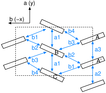
Figure 1: (Color online) Crystal structure on two-dimensional plane with four molecules A(1), A’(2), B(3), and C(4), in the unit cell where the respective bonds represent seven transfer energies $t_{b1},\cdots,t_{a3}$.

In Fig. 1, the crystal structure of $\alpha$-(BEDT-TTF)₂I₃ is shown where there are four sites, i.e., A, A’, B, and C, in the unit cell with an inversion symmetry between the A and A’ sites. For the insulating state, which is found at ambient pressure, the symmetry is broken since the electron density at the A site is different from that at the A’ site owing to a stripe charge ordering perpendicular to the stacking axis. [12, 13, 14, 15] At high pressures where the zero-gap state emerges, the symmetry is restored, and the electron density at the A site becomes equal to that at the A’ site. [16] The zero-gap state is robust to the variation in pressure, although the contact point moves in the Brillouin zone (BZ).[7] Small amounts of anion potential which are the same for the A and A’ sites but are different for the B and C sites, do not break the contact point of the Dirac cone. [17] These site potentials for B and C also stabilize the zero-gap state by reducing the overlap between the conduction and valence bands. [18] A pair of Dirac cones located at the incommensurate wave vector in the BZ is expected to vanish at high pressures by merging at a symmetric point (e.g., $\Gamma$ point). [19, 20, 21] Furthermore, it has been shown that the four sites, A, A’, B, and C provide the respective role for the tilted Dirac cone, and that each site gives a difference in the local density of states, as shown in the temperature dependence of the Knight shift and $T_{1}^{-1}$ of NMR. [17, 22]

Such a Dirac particle can be represented in terms of a reduced Hamiltonian with a 2x2 matrix instead of the original 4x4 matrix Hamiltonian, where the reduced Hamiltonian based on the Luttinger-Kohn (LK) representation, [23] gives the tilted Weyl equation [19, 11, 24] for the Dirac particle. The reduced model is successful to examine the novel property of transport phenomena, [11, 25, 26] which exhibit several differences from those of graphene, [27, 28] owing to tilting.

Although much progress has been achieved on the basis of the zero-gap state , [29, 30, 31] the condition for the Dirac particle is not yet clear since a contact point is formed owing to the accidental degeneracy in the energy band. [32] In the present study, as the next step in understanding the Dirac particle, we examine the Berry curvature[33, 34, 35] for the $\alpha$-(BEDT-TTF)₂I₃ salt, which comes from the property of the wave function. The curvature is also a useful tool for searching for the particle in other organic conductors. The Dirac particle has been maintained using a fact that the gap between the first band and the second band is zero within numerically accuracy. However, this is not always the case for the Dirac particle since there is also a Dirac particle with a gap, e.g., a massive Dirac particle in the low-energy model of boron nitride,[36] and also in the charge ordered state of $\alpha$-(BEDT-TTF)₂I₃ at pressures slightly lower than those of the zero-gap state. [37]

In §2, the formulation for the Berry curvature of $\alpha$-(BEDT-TTF)₂I₃ is given using a 4x4 Hamiltonian. To calculate the Berry curvature with a finite magnitude around the contact point, we add a small potential that differs between the A and A’ sites, based on the previous work. [38] Furthermore, a reduced Hamiltonian of a 2x2 matrix is examined by calculating the analytical property of the curvature. In §3, the Berry curvatures of the Dirac particle with multibands are studied numerically by taking a typical pressure, $P_{a}$ =6 kbar. Velocity fields and Berry curvature are also studied. The summary and discussion are given in §4.

2 Formulation and Hamiltonian

2.1 Berry curvature of multibands

We consider a two-dimensional electron system consisting of $M$ molecular sites in a unit cell where $M=4$ in the present case. The Schrödinger equation is given by

$$H(\bm{k})|n(\bm{k})>=E_{n}|n(\bm{k})>\;,$$ (1)

where $\bm{k}=(k_{x},k_{y})$ is a two-dimensional wave vector, and $n(=1,2,\cdots,M)$ denotes a band index. The quantities $H(\bm{k})$, $E_{n}(\bm{k})$, and $|n(\bm{k})>$ are the Hamiltonian with an MxM matrix for the $M$ sites, eigenvalue (band energy), and eigenfunction (wave function), respectively. When $\bm{k}(t)$ varies slowly with time $t$, the equation for motion is written as

$$i\hbar\partial_{t}|n(\bm{k}(t))>=H(\bm{k}(t))|n(\bm{k}(t))>.$$ (2)

When $\bm{k}$ moves along a closed loop C, the state $|n(\bm{k})>$ after returning to the original location is replaced by ${\rm e}^{i\gamma_{n}}|n(\bm{k})>$. The quantity $\gamma_{n}$ is the Berry phase given by [33]

$$\gamma_{n}= {\rm i}\int_{\rm C}\left<n(\bm{k})\cdot\bm{\nabla}_{\bm{k}}n(\bm{k})\right>{\rm d}\bm{k}=\int_{\rm S}\bm{B}_{n}(\bm{k})\cdot{\rm d}\bm{S},$$ (3)

where S is a region enclosed by the loop C. The vector field $\bm{B}_{n}(\bm{k})$ is the Berry curvature expressed as

$$\bm{B}_{n}(\bm{k}) =-{\rm Im}\left<\bm{\nabla}_{\bm{k}}n|\times|\bm{\nabla}_{\bm{k}}n\right>,$$ (4)

which is oriented perpendicularly to the $k_{x}$-$k_{y}$ plane. Noted that $\bm{B}_{n}=0$ for a single component owing to $<n|n>=1$.

The Berry curvature can be rewritten as [33]

$$\bm{B}_{n}(\bm{k}) =-{\rm Im}\sum_{m(\not=n)}\frac{\left<n|\bm{\nabla}_{\bm{k}}H|m\right>\times\left<m|\bm{\nabla}_{\bm{k}}H|n\right>}{(E_{m}-E_{n})^{2}}\;,$$ (5)

which is used for the numerical calculation. Note that

$$\sum_{n=1}^{4}\bm{B}_{n}(\bm{k})=0\;,$$ (6)

for an arbitrary $\bm{k}$ since $\left<n|\bm{\nabla}_{\bm{k}}H|m\right>$ is complex conjugate to $\left<m|\bm{\nabla}_{\bm{k}}H|n\right>$, and the double summations of $n$ and $m$ result in the vanishment of the imaginary part. This suggests a possible pair of Dirac cones located between two neighboring energy bands, because the singularity of one band must be compensated with that of the other band.

2.2 Hamiltonian for $\alpha$-(BEDT-TTF)₂I₃

The contact point, which is obtained in a normal state, i.e., without charge ordering, is determined essentially by the property of the transfer energy, and the effect of interaction is to modify mainly the location of the contact point (see Fig. 5 in ref. Kobayashi2007JPSJ). Then, by taking account of only transfer energy, we examine the Hamiltonian for $\alpha$-(BEDT-TTF)₂I₃ given by

$$\tilde{H}=\sum_{\alpha,\beta=1}^{4}\sum_{\sigma}\sum_{\bm{i},\bm{j}}^{\rm N}t_{\alpha,\beta;\bm{i},\bm{j}}a_{\alpha\sigma,\bm{i}}^{\dagger}a_{\beta\sigma,\bm{j}}\;,$$ (7)

where $\alpha,\beta$ (=1, 2, 3,4) are indices for the sites of molecules A (1), A’(2), B (3), and C (4) in the unit cell, and $\bm{i},\bm{j}(=\bm{R}_{i},\bm{R}_{j})$ are those for the cell forming a square lattice with N sites. The quantity $a_{\alpha,\bm{j}}^{\dagger}$ denotes the creation operator for the electron, and $t_{\alpha,\beta;\bm{i},\bm{j}}$ denotes the transfer energy between the neighboring site. As shown in Fig. 1, there are seven transfer energies given by $t_{b1}\cdots t_{b4}$ for the direction of the $b(-x)$-axis and by $t_{a1}\cdots t_{a3}$ for the direction of the $a(y)$-axis. We note that the definition of transfer energies in Fig. 1 (ref. Mori1984) differs from our previous one, $t_{p1},\cdots,t_{c4}$.[7] Since the two-dimensional plane of the previous one is reversed compared with that in Fig. 1, the relation is given by $t_{p1}=t_{b2}$, $t_{p2}=t_{b1}$, $t_{p3}=t_{b4}$, $t_{p4}=t_{b3}$, $t_{c1}=t_{a2}$, $t_{c2}=t_{a3}$, and $t_{c3}(=t_{c4})=t_{a1}$. In order to calculate the Berry curvature, which becomes finite around the Dirac point, we introduce site potentials $I_{\alpha\sigma}$ acting on A (1) and A’(2) differently in the form of

$$\tilde{H}_{\rm site}=\sum_{\alpha,\beta=1}^{4}\sum_{\bm{i},\bm{j}}^{\rm N}I_{\alpha\sigma}\delta_{\bm{i},\bm{j}}\delta_{\alpha,\beta}a_{\alpha,\sigma,\bm{i}}^{\dagger}a_{\beta,\sigma,\bm{j}}\;,$$ (8)

where

$$I_{1\sigma}=-I_{2\sigma}=-\Delta_{0},$$ (9)

and $I_{3\sigma}=I_{4\sigma}=0$. Equation (8) is a Hamiltonian of the site potential that creates a gap by breaking the inversion symmetry between A and A’.

Using the Fourier transform $a_{\alpha}(\bm{k})=\frac{1}{\sqrt{N}}\sum_{\bm{j}}a_{\alpha,\bm{j}}\exp[-i\bm{k}\cdot\bm{R}_{j}]$, the total Hamiltonian is expressed as

$$\tilde{H}+\tilde{H}_{\rm site} = \sum_{\bm{k}\sigma}\begin{pmatrix}a_{1\sigma}(\bm{k})^{\dagger},&a_{2\sigma}(\bm{k})^{\dagger},&a_{3\sigma}(\bm{k})^{\dagger},&a_{4\sigma}(\bm{k})^{\dagger}\end{pmatrix}H(\bm{k})\begin{pmatrix}a_{1\sigma}(\bm{k})\\ a_{2\sigma}(\bm{k})\\ a_{3\sigma}(\bm{k})\\ a_{4\sigma}(\bm{k})\end{pmatrix},$$ (10)

$$H({\bf k}) = \begin{pmatrix}-\Delta_{0}&t_{c1}+t_{c2}{\rm e}^{-ik_{y}}&t_{p1}-t_{p4}{\rm e}^{ik_{x}}&t_{p2}-t_{p3}{\rm e}^{ik_{x}}\\ t_{c1}+t_{c2}{\rm e}^{ik_{y}}&\Delta_{0}&t_{p4}{\rm e}^{ik_{y}}-t_{p1}{\rm e}^{i(k_{x}+k_{y})}&t_{p3}-t_{p2}{\rm e}^{ik_{x}}\\ t_{p1}-t_{p4}{\rm e}^{-ik_{x}}&t_{p4}{\rm e}^{-ik_{y}}-t_{p1}{\rm e}^{-i(k_{x}+k_{y})}&0&t_{c3}+t_{c4}{\rm e}^{-ik_{y}}\\ t_{p2}-t_{p3}{\rm e}^{-ik_{x}}&t_{p3}-t_{p2}{\rm e}^{-ik_{x}}&t_{c3}+t_{c4}{\rm e}^{ik_{y}}&0\end{pmatrix}$$

. (11)

The lattice constant is taken as unity. By diagonalizing eq. (11), we obtain four bands $E_{j}({\bf k})$ $(j=1,\cdots,4)$, where $E_{1}({\bf k})>E_{2}({\bf k})>E_{3}({\bf k})>E_{4}({\bf k})$. For $I_{\alpha\sigma}=0$ where the inversion symmetry between A and A’ is maintained, the zero-gap state between $E_{1}({\bf k})$ and $E_{2}({\bf k})$ is obtained at $\pm\bm{k}_{0}$, i.e., with the uniaxial pressure along the $a$-axis, $P_{a}$, being larger than 3 kbar.[7] In the present paper, we introduce a small but finite $\Delta_{0}$ that induces a small gap 2$\Delta$ between two upper bands. We call $\bm{k}_{0}$ the Dirac point where $\bm{k}_{0}$ for $\Delta_{0}=0$ gives the contact point, and $\bm{k}_{0}$ for $\Delta_{0}\not=0$ corresponds to the minimum of the gap between $E_{1}(\bm{k})$ and $E_{2}(\bm{k})$.

2.3 Reduced Hamiltonian

We analytically examine $\bm{B}_{1}$, which denotes the curvature for the first band $E_{1}$. The present numerical calculation shows that $\bm{B}_{1}$ in eq. (5) is essentially determined by $E_{1}$ and $E_{2}$, i.e., the effects of $E_{3}$ and $E_{4}$ on $\bm{B}_{1}$ are negligibly small. Thus, eq. (5) may be rewritten as

$$\bm{B}_{1}(\bm{k})= -{\rm Im}\frac{\left<1(\bm{k})|\bm{\nabla}_{\bm{k}}H|2(\bm{k})\right>\times\left<2(\bm{k})|\bm{\nabla}_{\bm{k}}H|1(\bm{k})\right>}{(E_{2}-E_{1})^{2}}$$

$$=\frac{2}{(E_{2}-E_{1})^{2}}(\bm{v}_{1}(\bm{k})\times\bm{v}_{2}(\bm{k})),$$ (12)

where $\bm{v}_{1}$ and $\bm{v}_{2}$ are the velocity fields defined by

$$\left<1(\bm{k})|\bm{\nabla}_{\bm{k}}H|2(\bm{k})\right>=\bm{v}_{1}(\bm{k})+{\rm i}\bm{v}_{2}(\bm{k})\;.$$ (13)

Although the velocities $\bm{v}_{1}$ and $\bm{v}_{2}$ depend on the choice of the relative phase between $|1(\bm{k})>$ and $|2(\bm{k})>$, the product of $\bm{v}_{1}\times\bm{v}_{2}$ is independent of the phase.

From eq. (13), one can reduce the 4x4 Hamiltonian to the 2x2 Hamiltonian for the energy bands $E_{1}$ and $E_{2}$. Instead of eq. (12) where the band basis on $\bm{k}$ is taken, the effective Hamiltonian is expressed using the LK basis, which is fixed at $\bm{k}^{\rm LK}(=\bm{k}_{0})$. The general form of the 2x2 Hamiltonian, $H^{\rm red}(\bm{k})$, is given by

$$H^{\rm red}(\bm{k})=H^{\rm LK}(\bm{k}) = \begin{pmatrix}f_{3}+f_{0}&f_{1}-if_{2}\\ f_{1}+if_{2}&-f_{3}+f_{0}\end{pmatrix}$$

$$=f_{0}+f_{1}\sigma_{1}+f_{2}\sigma_{2}+f_{3}\sigma_{3}\;.$$

The quantity $\sigma_{j}$ denotes the Pauli matrix and the coefficient $f_{j}$ (= $f_{j}(\bm{k})$) is given as the function of the two-dimensional wave vector $\bm{k}$. Although the term $f_{0}$ gives the effect of the tilting for the Dirac cone, [25] $f_{0}$ is irrelevant to $\bm{B}$ and is discarded hereafter. Substituting eq. (2.3) into eq. (12), we obtain the Berry curvature as (see Appendix)

$$\bm{B}=-\frac{1}{2E^{3}}\left(f_{3}(\bm{\nabla}_{\bm{k}}f_{1}\times\bm{\nabla}_{\bm{k}}f_{2})+f_{1}(\bm{\nabla}_{\bm{k}}f_{2}\times\bm{\nabla}_{\bm{k}}f_{3})\right.$$

$$\left.+f_{2}(\bm{\nabla}_{\bm{k}}f_{3}\times\bm{\nabla}_{\bm{k}}f_{1})\right),$$ (15)

where $E=\sqrt{f_{1}^{2}+f_{2}^{2}+f_{3}^{2}}$.

Now, we examine the Berry curvature close to the Dirac point $\bm{k}_{0}$ using the LK basis at $\bm{k}^{\rm LK}$. The quantity $f_{j}(\bm{k})$ is expanded as

$$f_{1}(\bm{k})\simeq\bm{v}^{0}_{1}\cdot\bm{q},$$

$$f_{2}(\bm{k})\simeq\bm{v}^{0}_{2}\cdot\bm{q},$$

$$f_{3}(\bm{k})\simeq-\Delta,$$ (16)

where $\bm{q}=\bm{k}-\bm{k}^{\rm LK}$, $\bm{v}^{0}_{j}(=\bm{\nabla}_{\bm{k}}f_{j})$ is estimated at $\bm{k}=\bm{k}^{\rm LK}$, and the linear term in $f_{3}$ is absent. The quantity $2\Delta(<2\Delta_{0})$, which is the gap between the two bands of $E_{1}$ and $E_{2}$, is small compared with the bandwidth. From eqs. (15) and (16), the Berry curvature and Berry phase are respectively obtained as

$$\bm{B}=\frac{\Delta}{2E^{3}}\left(\bm{v}^{0}_{1}\times\bm{v}^{0}_{2}\right),$$ (17)

$$\gamma_{1}=\int(\bm{e}_{z}\cdot\bm{B}){\rm d}\;\bm{q}=\pi\frac{\bm{e}_{z}\cdot(\bm{v}^{0}_{1}\times\bm{v}^{0}_{2})}{|\bm{e}_{z}\cdot(\bm{v}^{0}_{1}\times\bm{v}^{0}_{2})|},$$ (18)

where $E=\sqrt{f_{1}^{2}+f_{2}^{2}+\Delta^{2}}$ and $\bm{e}_{z}$ denotes the unit vector perpendicular to the $q_{x}$-$q_{y}$ plane. In deriving eq. (18), the two-dimensional integral is extended to infinity.

Now, we examine the variation in the velocity fields around the Dirac point for an arbitrary $\bm{k}(\not=\bm{k}^{\rm LK}$) using eq. (13). By considering the case of

$$\bm{v}^{0}_{1}\rightarrow(v,0),\;\;\;\bm{v}^{0}_{2}\rightarrow(0,v^{\prime})\;\;\;{\rm and}\;\;\;f_{3}\rightarrow-\Delta,$$ (19)

we obtain (see eqs. (A) and (A) in Appendix)

$$\bm{v}_{1}(\theta_{\bm{q}})=\frac{\Delta}{E\sqrt{E^{2}-\Delta^{2}}}(v^{2}q_{x}\bm{e}_{x}+(v^{\prime})^{2}q_{y}\bm{e}_{y})\;,$$ (20)

$$\bm{v}_{2}(\theta_{\bm{q}})=\frac{1}{\sqrt{E^{2}-\Delta^{2}}}vv^{\prime}(-q_{y}\bm{e}_{x}+q_{x}\bm{e}_{y})\;,$$ (21)

$$\bm{B}=\frac{\Delta vv^{\prime}}{2E^{3}}\bm{e}_{z}\;,$$ (22)

where $E=\sqrt{v^{2}q_{x}^{2}+v^{\prime 2}q_{y}^{2}+\Delta^{2}}$. These velocity fields rotate around $\bm{k}_{0}$ as shown explicitly for the 4x4 Hamiltonian in the next section.

Here, we comment on the reduced Hamiltonian of eq. (19) rewritten as

$$H^{(I)}= \begin{pmatrix}-\Delta&q_{x}-iq_{y}\\ q_{x}+iq_{y}&\Delta\end{pmatrix}=q_{x}\sigma_{1}+q_{y}\sigma_{2}-\Delta\sigma_{3}\;,$$

where $v=v^{\prime}=1$. By introducing a unitary transformation, eq. (LABEL:eq:Koba_KT) is transformed as follows. The transformation for ${\rm e}^{-i\sigma_{2}\phi/2}$ with $\phi=\pi/2$ gives

$$H^{(II)}= {\rm e}^{-i\sigma_{2}\phi/2}H^{(I)}{\rm e}^{i\sigma_{2}\phi/2}$$

$$=\begin{pmatrix}q_{x}&\Delta-iq_{y}\\ \Delta+iq_{y}&-q_{x}\end{pmatrix}=\Delta\sigma_{1}+q_{y}\sigma_{2}+q_{x}\sigma_{3}\;,$$

and that for ${\rm e}^{i\sigma_{1}\phi/2}$ with $\phi=\pi/2$ gives

$$H^{(III)}= {\rm e}^{i\sigma_{1}\phi/2}H^{(I)}{\rm e}^{-i\sigma_{1}\phi/2}$$

$$=\begin{pmatrix}k_{y}&k_{x}-i\Delta\\ k_{x}+i\Delta&-k_{y}\end{pmatrix}=k_{x}\sigma_{1}+\Delta\sigma_{2}+k_{y}\sigma_{3}\;.$$

For $\Delta=0$, eqs. (LABEL:H:Kata) and (LABEL:H:Koba_Hall) are reduced to those derived by Katayama et al.[17] and Kobayashi et al.[11], respectively, who chose different bases for the L-K state with $\bm{v}^{0}_{1}$ and $\bm{v}^{0}_{2}$ being orthogonal. Note that all these cases lead to $B_{z}=\bm{B}\cdot\bm{e}_{z}=\Delta/(2E^{3})$ owing to the rotation that does not depend on $\bm{q}$.

3 Berry Curvature for $\alpha$-(BEDT-TTF)₂I₃

To calculate the Berry phase of the conductor under uniaxial $P_{a}$ along the stacking axis, we use an extrapolation[5] for $t_{\alpha\beta}$ given by [4]

$$t_{\alpha\beta}(P_{a})=t_{\alpha\beta}(0)+C_{\alpha\beta}P_{a}\;.$$ (26)

The unit of energy is taken as eV and that of pressure $P_{a}$ is taken as kbar. Equation (26) corresponding to $\alpha$-(BEDT-TTF)₂I₃ gives the zero-gap state for $P_{a}>3$ kbar. We perform the calculation by taking $P_{a}$ = 6 kbar and $\Delta_{0}=$ 0.02 eV. The gap on the Dirac point ${\bf k}_{0}$, i.e., $2\Delta(\simeq$ 0.02 eV), is smaller than $2\Delta_{0}$.

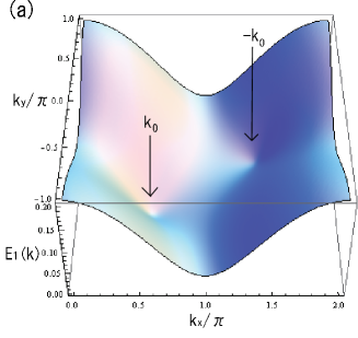
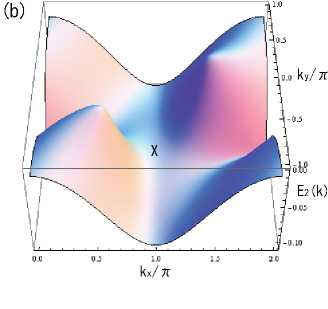
Figure 2: (Color online) Energy bands of $E_{1}(\bm{k})$ (a) and $E_{2}(\bm{k})$ (b) for $P_{a}=6$ kbar and $\Delta_{0}=$0.02 eV, where the regions for the $k_{x}$ and $k_{y}$ axes are given as $0<k_{x}<2\pi$ and $-\pi<k_{y}<\pi$. The arrow denotes the location for the Dirac point at ${\bf k}_{0}=(0.57\pi,-0.30\pi)$ where the gap between $E_{1}(\bm{k})$ and $E_{2}(\bm{k})$ is estimated as $2\Delta\simeq$ 0.02 eV. Two cones are situated symmetrically with respect to the X point $(\pi,0)$ and the $\Gamma$ point $(0,0)$.

Figure 3: (Color online) Berry curvature and the contour plot of $-\bm{B}\cdot\bm{e}_{z}$ for the energy band $E_{1}(\bm{k})$ on the $k_{x}$-$k_{y}$ plane corresponding to Fig. 1(a), where $\bm{e}_{z}$ denotes the unit vector perpendicular to $k_{x}$-$k_{y}$ plane. The middle of the horizontal axis (vertical axis) in the contour plot denotes the M (${\rm\Gamma}$)) point.

The energy bands $E_{1}$ and $E_{2}$ are shown in Figs. 2(a) and 2(b), respectively. The Dirac cone exists at ${\bf k}\simeq\pm{\bf k}_{0}$ with ${\bf k}_{0}=(0.57\pi,-0.3\pi)$, which is shown by an arrow. A pair of cones is seen around $E_{1}({\bf k}_{0})$ and $E_{2}({\bf k}_{0})$, and the cones in the same band are symmetric with respect to the $\Gamma$(=(0,0)) point. For $E_{1}(\bm{k})$, the maximum is seen at the Y(=$(0,\pm\pi)$) point while saddle points are seen for the X(=$(\pi,0)$), M(=$(\pi,\pm\pi)$), and $\Gamma$ points. For $E_{2}(\bm{k})$, the minimum is seen at the M point while saddle points are seen for the X, Y, and $\Gamma$ points. The accidental degeneracy, which is found at $\pm\bm{k}_{0}$ for $\Delta_{0}\rightarrow 0$, is realized as the minimum of $E_{1}(\bm{k})$ and the maximum of $E_{2}(\bm{k})$.

The Berry curvature, which is calculated using eq. (5), is shown in Figs. 3(a) and 3(b) for the three-dimensional (3D) view on the $k_{x}$-$k_{y}$ plane (a), and for the contour plot (b). The peak around $-\bm{k}_{0}$ ( $\bm{k}_{0}$) is positive (negative). They are antisymmetric with respect to the $\Gamma$ point (the middle point on the vertical axis). Since the curvature exhibits a noticeable peak close to $\bm{k}_{0}$, such a peak may be identified as the Dirac particle instead of calculating the contact point. We note that a quantity called a Chern number [39] is given by

$$\frac{1}{2\pi}\int_{S}{\rm d}{S}\;\bm{B}\cdot\bm{e}_{z}=0,$$ (27)

owing to the time reversal symmetry, i.e., $\bm{B}(-\bm{k})=-\bm{B}(\bm{k})$, where $S$ denotes the total BZ. In Fig. 3(a), the curvature around the Dirac point is slightly anisotropic in the sense that it is slightly extended to the $y$-direction. With increasing pressure, the difference is reduced and the curvature becomes almost isotropic at $P_{a}$ = 10 kbar, where two Dirac particles are well isolated.

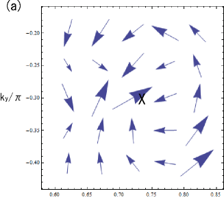
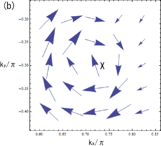
Figure 4: (Color online) Vector fields of velocities $-\bm{v}_{1}$ (a) and $-\bm{v}_{2}$ (b) on the $k_{x}$-$k_{y}$ plane around the Dirac point, $\bm{k}_{0}$,(cross) in Fig. 2.

Using eq. (13), we examine velocity field as a function of $\bm{k}$. In Figs. 4(a) and 4(b), the $\bm{k}$ dependence of the velocities $\bm{v}_{1}$ and $\bm{v}_{2}$ around $\bm{k}_{0}$ are shown. Since the phases of both $|1(\bm{k})>$ and $|2({k})>$ are arbitrary, we choose them so that both of their first components corresponding to the A site are real. We verified that $\bm{B}$ calculated in terms of $\bm{v}_{1}(\bm{k})\times\bm{v}_{2}(\bm{k})$ in eq.(12) reproduces well the result in Fig. 3 within numerical accuracy. Both $\bm{v}_{1}$ and $\bm{v}_{2}$, which are almost orthogonal, rotate around the Dirac point, indicating the singularity at $\bm{k}_{0}$. The vortex structure around the Dirac point is also understood from eqs. (20) and (21). Even in the presence of the site potential $\Delta_{0}$, which removes the degeneracy of the zero-gap state, the existence of such vortex behavior suggests a topological property of the Dirac particle.

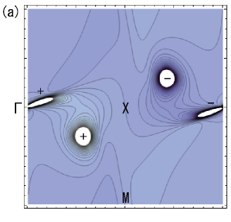
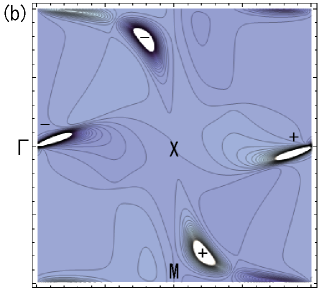
Figure 5: (Color online) Contour plot of Berry curvature, $B(\Delta_{0})$, for energy bands $E_{2}(\bm{k})$ (a) and $E_{3}(\bm{k})$ (b).

Here, we examine the Berry curvature for other bands of $E_{2}(\bm{k})$, $E_{3}(\bm{k})$, and $E_{4}(\bm{k})$. The Berry curvature of the second band $E_{2}(\bm{k})$ is shown in Fig. 5(a). The peak located at $\pm\bm{k}_{0}$ has a sign opposite to that of $E_{1}(\bm{k})$. In addition to such a peak, another pair of peaks appears close to the $\Gamma$ point. The latter one is rather extended to a direction slightly declined toward the horizontal axis, suggesting a large anisotropy of the Dirac cone. The anisotropic peak disappears for a small $P_{a}<$ 3 kbar while it becomes rather isotropic for a large $P_{a}$. Such a behavior resembles the emergence of the Dirac particle in the charge ordered state, which has been shown in $\alpha$-(BEDT-TTF)₂I₃.[37] In Fig. 5(b), the Berry curvature for $E_{3}(\bm{k})$ is shown. A pair of peaks close to the $\Gamma$ point also shows a sign opposite to that of $E_{2}(\bm{k})$. There is another peak close to the M point, which compensates for that of $E_{4}(\bm{k})$ (not shown here). These results show that each neighboring band provides a pair of Dirac particles followed by the Berry curvature with an opposite sign. When one pair of Dirac particles between neighboring bands is found, one may expect another pair between neighboring bands.

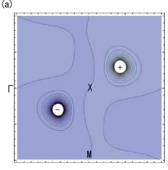
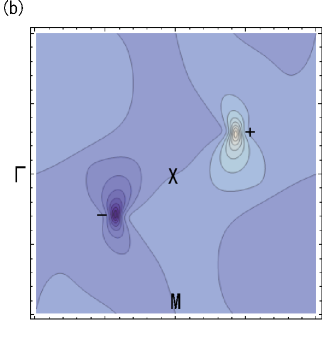
Figure 6: (Color online) Contour plots of the Dirac component of eq. (29) (a), and the background component of eq. (30) (b), for Berry curvature of $E_{1}(\bm{k})$ in Fig. 3.

Since the Berry curvature $\bm{B}(\bm{k})$ in Fig. 3 depends on the sign of the site potential $\pm\Delta_{0}$, we examine $\bm{B}(\bm{k})$ by dividing it into two components, i.e., $B_{\rm Dirac}$ and $B_{\rm back}$, which are symmetric and antisymmetric, respectively, with respect to $\Delta_{0}$. By defining

$$B(\Delta_{0})=\bm{B}_{1}(\bm{k},\Delta_{0})\cdot\bm{e}_{z}\;,$$ (28)

these components are rewritten as

$$B_{\rm Dirac} =\frac{B(\Delta_{0})-B(-\Delta_{0})}{2}\;,$$ (29)

$$B_{\rm back} =\frac{B(\Delta_{0})+B(-\Delta_{0})}{2}\;.$$ (30)

The first one is related to the topological property, which does not depend on the details of the energy band. The second one depends on the property of the energy band. The curvatures given by eqs. (29) and (30) are shown in Figs. 6(a) and 6(b), respectively. The peak height of $B_{\rm Dirac}$ is $10^{2}$ times as much as that of $B_{\rm back}$. When $\Delta_{0}$ decreases to zero, $B_{\rm Dirac}$ increases rapidly, but $B_{\rm back}$ remains almost unchanged. The component $B_{\rm Dirac}$ is located in the narrow region around $\pm\bm{k}_{0}$, suggesting a character of the Dirac particle. The component $B_{\rm back}$, which is small and spreads in the entire region of the BZ, is irrelevant to the Dirac particle. Thus, the separation of $B_{\rm Dirac}$ from $B(\Delta_{0})$ gives the intrinsic curvature of the Dirac particle.

Figure 7: $\Delta_{0}$ dependence of $\Omega_{\rm Dirac}$ (eq. (31)), $\Omega_{\rm back}$, (eq. (32)), $\Omega{\rm abs}$ (eq. (33)), and gap $2\Delta$ .

To estimate the magnitude of the peak of $B(\bm{k},\Delta_{0})$, we examine the following integrated quantities of the respective components:

$$\Omega_{\rm Dirac} =\frac{1}{2\pi}\int_{S}{\rm d}{S}\;{\rm sgn}(k_{y})\frac{B(\Delta_{0})-B(-\Delta_{0})}{2}\;,$$ (31)

$$\Omega_{\rm back} =\frac{1}{2\pi}\int_{S}{\rm d}{S}\;{\rm sgn}(k_{y})\frac{B(\Delta_{0})+B(-\Delta_{0})}{2}\;.$$ (32)

The quantity $\Omega_{\rm Dirac}+\Omega_{\rm back}$ is a Berry phase where $S$ in eq. (3) is the region given by $-\pi<k_{x}<\pi$ and $0<k_{y}<\pi$. The quantity $\Omega_{\rm Dirac}$ comes from the contribution of the Dirac cone with a singularity, and the second one originates from the property of the conventional band. Note that $\Omega_{\rm Dirac}$ remains the same but $\Omega_{\rm back}$ varies when we replace ${\rm sgn}(k_{y})$ by ${\rm sgn}(k_{x})$ in the limit of small $\Delta_{0}$. In Fig. 7, $\Omega_{\rm Dirac}$ and $\Omega_{\rm back}$ are shown as the function of $\Delta_{0}$. With decreasing $\Delta_{0}$, $\Omega_{\rm Dirac}$ is reduced to 1, since the boundary effect of BZ becomes negligible. This indicates the intrinsic property of Dirac cones. We also show the quantity

$$\Omega_{\rm abs} =\frac{1}{2\pi}\int_{S}{\rm d}{S}\;\frac{|B(\Delta_{0})|+|B(-\Delta_{0})|}{2}.$$ (33)

Note that $\Omega_{\rm abs}$ is larger than $\Omega_{\rm Dirac}$ and $\Omega_{\rm back}$, and becomes even larger than 1 for a small $\Delta_{0}$. The enhancement of $\Omega_{\rm abs}$ is attributable to the alternation of the sign of $B(\Delta_{0})$ as a function of ${\bf k}$, which originates from the background property of the band structure.

4 Summary and discussion

We obtained the following for the Berry curvature of $\alpha$-(BEDT-TTF)₂I₃, which exhibits the zero-gap state under the uniaxial pressure.

(i) In the present study, instead of the zero gap between $E_{1}(\bm{k})$ and $E_{2}(\bm{k})$, the Dirac particle is examined by calculating the Berry curvature for the 4x4 Hamiltonian. By adding a small potential $\Delta_{0}$ acting on the A and A’ sites with opposite signs, which breaks the inversion symmetry, the Dirac particle is identified by the pronounced peak of the Berry curvature in the same band, and also between neighboring bands. The Berry curvature consists of two components,i.e., $B_{\rm Dirac}$ and $B_{\rm back}$, where $B_{\rm Dirac}$ ($B_{\rm back}$) is an odd (even) function with respect to $\Delta_{0}$. The peak in $B_{\rm Dirac}$, which is located close to the Dirac cone, is intrinsic to the Dirac particle. The quantity $B_{\rm back}$, which is small but is extended in the whole BZ, is irrelevant to the Dirac particle. The latter could be the origin of the curvature, which depends on the choice of the phase in the transfer integrals of the site Hamiltonian. [40]

(ii) The Berry curvature is calculated in the general case of the reduced 2x2 Hamiltonian. Once such Hamiltonian (i.e., the coefficient of Pauli matrices) for other organic conductors with possible Dirac particles is obtained on the L-K basis, eq. (15) is applicable to understand the characteristic behavior of the Berry curvature. The Berry curvature is determined by a vector product of two types of velocity fields, which are given as the coefficients of the Pauli matrices, $\sigma_{1}$ and $\sigma_{2}$, in the reduced Hamiltonian. These velocity fields rotate around the Dirac point as a vortex and are determined uniquely, except for the Dirac point.

(iii) We found a pair of Dirac particles not only between $E_{1}(\bm{k})$ and $E_{2}(\bm{k})$ , but also between the other neighboring band, although the mutual relation of these Dirac points is unclear owing to the accidental degeneracy. In the present case, the curvature between $E_{2}(\bm{k})$ and $E_{3}(\bm{k})$ exhibits a behavior close to merging. It is possible that a pair of Dirac particles may exist in many neighboring bands, if a pair of peaks is found in one band.

Here, we comment on the effect of a short-range repulsive interaction on the Dirac particle. In the presence of the interaction that also gives the normal state, i.e., no gap, the critical pressure for the zero-gap state ($P_{a}\sim 4$ kbar) [19] is larger than that in the absence of interaction ($P_{a}\sim 3$ kbar), suggesting that the interaction suppresses the zero-gap state. Such an effect appears as the on-site potential acting on the B and C sites. Comparing the Berry curvature in Fig. 3(a) with that in the presence of the interaction (not shown here), we found that the Berry curvature in the presence of the interaction becomes rather anisotropic and exhibits a small tail toward the M-point, indicating a tendency toward merging. Thus, merging may occur owing to the interaction, in addition to the variation in the transfer energy. [7] Note that the pair of Dirac particles already merges at the M-point in the charge ordering state at ambient pressure, which was obtained in our previous study.[5]

At present, it is not yet clear how Dirac particles emerge in organic conductors, since it occurs accidentally in the BZ. However, the calculation of the Berry curvature is a useful tool for searching Dirac particles particularly in the multiband system even when the symmetry is broken or when the band structure is complicated. Actually, it is shown that the organic conductor $\alpha$-(BEDT-TTF)₂NH₄Hg(SCN)₄ with a complicated band structure exhibits Dirac particles with a zero gap under pressure.[41] In the case where the symmetry is broken, the formation of massive Dirac particles in the stripe charge ordered state is reported in a separate paper. [37]

Appendix A Berry curvature and velocity field for general Hamiltonian

We calculate the Berry curvature for the reduced 2x2 Hamiltonian given by (eq. (2.3)),

$$H^{\rm LK}(\bm{k}) =\begin{pmatrix}f_{3}&f_{1}-if_{2}\\ f_{1}+if_{2}&-f_{3}\end{pmatrix},$$ (34)

where the quantity $\sigma_{j}$ denotes the Pauli matrix and the energy is measured from the chemical potential. The quantity $f_{j}$ (= $f_{j}(\bm{k})$) depends on the two-dimensional wave vector $\bm{k}(=\bm{k}_{0}+\bm{q})$. The Schrödinger equation for the Hamiltonian (34) is written as

$$H^{\rm red}\Psi_{\pm}=\pm E\Psi_{\pm},$$ (35)

where $\Psi_{+}=|1(\bm{k})>_{0}$, $\Psi_{-}=|2(\bm{k})>_{0}$. The energy and wave function are calculated as

$$E=\sqrt{f_{1}^{2}+f_{2}^{2}+f_{3}^{2}}\;,$$ (36)

$$\Psi_{\pm}=\frac{1}{\sqrt{2E(E\mp f_{3})}}\begin{pmatrix}f_{1}-if_{2}\\ \pm E-f_{3}\end{pmatrix}\equiv\begin{pmatrix}\tilde{f}_{1}(\bm{k})-i\tilde{f}_{2}(\bm{k})\\ g_{\pm}(\bm{k})\end{pmatrix}.$$ (37)

The relative phase between $\Psi_{+}$ and $\Psi_{-}$ is undetermined and is chosen such that the second component of each state is real and positive.

Now, we calculate $\bm{B}_{1}$ for $\Psi_{+}$ explicitly using eq. (4). By noting that only the first component contains the imaginary part, the Berry curvature $\bm{B}(\bm{k})$ is calculated as

$$\bm{B_{1}} =\bm{B}=-{\rm Im}\left(\bm{\nabla}_{\bm{k}}\Psi_{+}^{\dagger}\right)^{t}\times\left(\bm{\nabla}_{\bm{k}}\Psi_{+}\right)$$

$$=-{\rm Im}(\bm{\nabla}_{\bm{k}}\tilde{f}_{1}+i\bm{\nabla}_{\bm{k}}\tilde{f}_{2})\times(\bm{\nabla}_{\bm{k}}\tilde{f}_{1}-i\bm{\nabla}_{\bm{k}}\tilde{f}_{2})=2\bm{\nabla}_{\bm{k}}\tilde{f}_{1}\times\bm{\nabla}_{\bm{k}}\tilde{f}_{2}\;,$$ (38)

where

$$\bm{\nabla}_{\bm{k}}\tilde{f}_{1}= \frac{1}{\sqrt{2E(E-f_{3})}}\{(1-\frac{(2E-f_{3})f_{1}^{2}}{2E^{2}(E-f_{3})}\bm{\nabla}_{\bm{k}}f_{1}$$

$$-\frac{(2E-f_{3})f_{2}f_{1}}{2E^{2}(E-f_{3})}\bm{\nabla}_{\bm{k}}f_{2}+\frac{(E-f_{3})f_{1}}{2E^{2}}\bm{\nabla}_{\bm{k}}f_{3}\}\;,$$ (39)

and

$$\bm{\nabla}_{\bm{k}}\tilde{f}_{2}= \frac{1}{\sqrt{2E(E-f_{3})}}\{-\frac{(2E-f_{3})f_{2}f_{1}}{2E^{2}(E-f_{3})}\bm{\nabla}_{\bm{k}}f_{1}$$

$$+(1-\frac{(2E-f_{3})f_{2}^{2}}{2E^{2}(E-f_{3})}\bm{\nabla}_{\bm{k}}f_{2}+\frac{(E-f_{3})f_{2}}{2E^{2}}\bm{\nabla}_{\bm{k}}f_{3}\}.$$ (40)

Substituting eqs. (39) and (40) into eq. (38), we obtain eq. (15).

Note that eq. (15) can also be obtained from eq. (5), which is rewritten as

$$\bm{B} =-{\rm Im}\left\{(\Psi_{+}^{\dagger}\bm{\nabla}_{\bm{k}}H\Psi_{-})\times(\Psi_{-}^{\dagger}\bm{\nabla}_{\bm{k}}H\Psi_{+})\frac{1}{4E^{2}}\right\}=-\frac{1}{4E^{2}}\times$$

$${\rm Im}\left\{\right.(\Psi_{+}|\sigma_{1}\bm{\nabla}_{\bm{k}}f_{1}+\sigma_{2}\bm{\nabla}_{\bm{k}}f_{2}+\sigma_{3}\bm{\nabla}_{\bm{k}}f_{3}|\Psi_{-})\times(\Psi_{-}|\sigma_{1}\bm{\nabla}_{\bm{k}}f_{1}+\sigma_{2}\bm{\nabla}_{\bm{k}}f_{2}+\sigma_{3}\bm{\nabla}_{\bm{k}}f_{3}|\Psi_{+})\left.\right\},$$ (41)

where $(\Psi_{\pm}|=(\tilde{f}_{1}+i\tilde{f}_{2},g_{\pm})^{t}$. Equation (41) is calculated as eq. (15) by noting $(\Psi_{-}|\sigma_{1}|\Psi_{+})=-(f_{3}f_{1}-{\rm i}Ef_{2})/(E\sqrt{E^{2}-f_{3}^{2}})$, $(\Psi_{-}|\sigma_{2}|\Psi_{+})=-(f_{3}f_{2}+{\rm i}Ef_{1})/(E\sqrt{E^{2}-f_{3}^{2}})$, and $(\Psi_{-}|\sigma_{3}|\Psi_{+})=\sqrt{E^{2}-f_{3}^{2}}/E$.

Here, we calculate the velocity field defined by eq. (13). Substituting eq. (37) into eq. (13), we obtain

$$\bm{v}_{1}(\theta_{\bm{k}})= {\rm Re}\{\Psi^{\dagger}_{-}\bm{\nabla}_{\bm{k}}H^{\rm LK}\Psi_{+}\}$$

$$=\frac{-1}{E\sqrt{E^{2}-f_{3}^{2}}}\Large(f_{3}(f_{1}\bm{\nabla}_{\bm{k}}f_{1}+f_{2}\bm{\nabla}_{\bm{k}}f_{2})$$

$$-(f_{1}^{2}+f_{2}^{2})\bm{\nabla}_{\bm{k}}f_{3}\Large),$$ (42)

$$\bm{v}_{2}(\theta_{\bm{k}})= {\rm Im}\{\Psi_{-}\bm{\nabla}_{\bm{k}}H^{\rm LK}\Psi_{+}\}$$

$$=\frac{-1}{\sqrt{E^{2}-f_{3}^{2}}}\Large(-f_{2}\bm{\nabla}_{\bm{k}}f_{1}+f_{1}\bm{\nabla}_{\bm{k}}f_{2}\Large)\;,$$ (43)

$$\bm{v}_{3}(\theta_{\bm{k}})= \frac{1}{2}\{\Psi^{\dagger}_{+}\bm{\nabla}_{\bm{k}}H^{\rm LK}\Psi_{+}-\Psi^{\dagger}_{-}\bm{\nabla}_{\bm{k}}H^{\rm LK}\Psi_{-}\}$$

$$=\frac{1}{\sqrt{E^{2}-f_{3}^{2}}}\Large(f_{1}\bm{\nabla}_{\bm{k}}f_{1}+f_{2}\bm{\nabla}_{\bm{k}}f_{2}+f_{3}\bm{\nabla}_{\bm{k}}f_{3}\Large)\;.$$ (44)

Substituting eqs. (A) and (A) into eq. (12), one finds that $\bm{B}_{1}$ is exactly the same as eq.(15).

References

- [1] T. Mori, A. Kobayashi, T. Sasaki, H. Kobayashi, G. Saito, and H. Inokuchi: Chem. Lett. (1984) 957.
- [2] K. Kajita, T. Ojiro, H. Fujii, Y. Nishio, H. Kobayashi, A. Kobayashi, and R. Kato: J. Phys. Soc. Jpn. 61 (1992) 23.
- [3] N. Tajima, A. Ebina-Tajima. M. Tamura, Y. Nishio, and K. Kajita: J. Phys. Soc. Jpn. 71 (2002) 1832.
- [4] R. Kondo, S. Kagoshima, and J. Harada: Rev. Sci. Instrum. 76 (2005) 093902.
- [5] A. Kobayashi, S. Katayama, and Y. Suzumura: J. Phys. Soc. Jpn. 73 (2004) 543.
- [6] A. Kobayashi, S. Katayama, K. Noguchi, and Y. Suzumura: J. Phys. Soc. Jpn. 73 (2004) 543.
- [7] S. Katayama, A. Kobayashi, and Y. Suzumura: J. Phys. Soc. Jpn. 75 (2006) 054705.
- [8] H. Kino and T. Miyazaki: J. Phys. Soc. Jpn. 75 (2006) 034704.
- [9] S. Ishibashi, T. Tamura, M. Kohyama, and K. Terakura: J. Phys. Soc. Jpn. 75 (2006) 015005.
- [10] N. Tajima, S. Sugawara, M. Tamura, R. Kato, Y. Nishio, and K. Kajita: EPL 80 (2007) 47002.
- [11] A. Kobayashi, Y. Suzumura, and H. Fukuyama: J. Phys. Soc. Jpn 77 (2008) 064718.
- [12] H. Seo, C. Hotta, and H. Fukuyama: Chem. Rev. 104 (2004) 5005.
- [13] H. Seo: J. Phys. Soc. Jpn. 69 (2000) 805.
- [14] H. Kino and H. Fukuyama: J. Phys. Soc. Jpn. 64 (1995) 4523.
- [15] T. Takahashi: Synth. Met. 133-134 (2003) 261.
- [16] T. Kakiuchi, Y. Wakabayashi, H. Sawa, T. Takahashi, and T. Nakamura: J. Phys. Soc. Jpn. 76 (2007) 113702.
- [17] S. Katayama, A. Kobayashi, and Y. Suzumura: Eur. Phys. J. B. 67 (2009) 139.
- [18] R. Kondo, S. Kagoshima, T. Naoya, and R. Kato: J. Phys. Soc. Jpn. 78 (2009) 114714.
- [19] A. Kobayashi, S. Katayama, Y. Suzumura, and H. Fukuyama: J. Phys. Soc. Jpn. 76 (2007) 034711.
- [20] G. Montambaux, F. Pichon, J.-N. Fuchs, and M. O. Goerbig: Eur. Phys. J. B 72 (2009) 509.
- [21] G. Montambaux, F. Pichon, J.-N. Fuchs, and M. O. Goerbig: Phys. Rev. B 80 (2009) 153412.
- [22] Y. Takano, K. Hiraki, Y. Takada, H. M. Yamamoto, and T. Takahashi: J. Phys. Soc. Jpn. 79 (2010) 104604.
- [23] J. M. Luttinger and W. Kohn: Phys. Rev. 97 (1955) 869.
- [24] M. O. Goerbig, J.-N. Fuchs, G. Montambaux, and F. Pichon: Phys. Rev. B 78 (2008) 045415.
- [25] A. Kobayashi, Y. Suzumura, H. Fukuyama, and M. O. Goerbig: J. Phys. Soc. Jpn 78 (2009) 114711.
- [26] T. Nishine, A. Kobayashi, and Y. Suzumura: J. Phys. Soc. Jpn. 79 (2010) 114715.
- [27] T. Ando: J. Phys. Soc. Jpn 74 (2005) 777.
- [28] K. S. Novoselov, A. K. Geim, S. V. Morozov, D. Jiang, M. I. Katsnelson, I. V. Grigorieva, S. V. Dubonos, and A. A. Firsov: Nature 438 (2005) 197.
- [29] N. Tajima, S. Sugawara, M. Tamura, Y. Nishio, and K. Kajita: J. Phys. Soc. Jpn. 75 (2006) 051010.
- [30] N. Tajima and K. Kajita: Sci. Technol. Adv. Mater. 10 (2009) 024308.
- [31] A. Kobayashi, S. Katayama, and Y. Suzumura: Sci. Technol. Adv. Mater. 10 (2009) 024309.
- [32] C. Herring: Phys. Rev. 52 (1937) 365.
- [33] M. V. Berry: Proc. R. Soc. Lond. A 392 (1984) 45.
- [34] Y. Aharonov and J. Anandan: Phys. Rev. Lett. 58 (1987) 1953.
- [35] D. Xiao, M.C. Chang, and Q. Niu: arXiv 0907.202.
- [36] J.-N. Fuchs, F. Pichon, M. O. Goerbig, and G. Montambaux: Eur. Phys. J B 77 (2010) 351.
- [37] A. Kobayashi, Y. Suzumura, F. Pichon, and G. Montambaux: to be published in Phys. Rev. B. (arXiv:1107.4841)
- [38] A. Kobayashi, S. Komaba, S. Katayama, and Y. Suzumura: J. Phys. Conf. Series 132 (2008) 012002.
- [39] D. J. Thouless, Topological Quantum Numbers in Nonrelativistic Physics (World Scientific, Singapore, 1998).
- [40] C. Bena and G. Montambaux: New J. Physics 11 (2009) 095003.
- [41] T. Choji, A. Kobayashi and Y. Suzumura: J. Phys. Soc. Jpn. 80 (2011) 074712.