Constructing EOB dynamics with numerical energy flux for intermediate-mass-ratio inspirals

Abstract

A new scheme for computing dynamical evolutions and gravitational radiations for intermediate-mass-ratio inspirals (IMRIs) based on an effective one-body (EOB) dynamics plus Teukolsky perturbation theory is built in this paper. In the EOB framework, the dynamics essentially affects the resulted gravitational waveform for binary compact star system. This dynamics includes two parts. One is the conservative part which comes from effective one-body reduction. The other part is the gravitational back reaction which contributes to the shrinking process of the inspiral of binary compact star system. Previous works used analytical waveform to construct this back reaction term. Since the analytical form is based on post-Newtonian expansion, the consistency of this term is always checked by numerical energy flux. Here we directly use numerical energy flux by solving the Teukolsky equation via the frequency-domain method to construct this back reaction term. And the conservative correction to the leading order terms in mass-ratio is included in the deformed-Kerr metric and the EOB Hamiltonian. We try to use this method to simulate not only quasi-circular adiabatic inspiral but also the nonadiabatic plunge phase. For several different spinning black holes, we demonstrate and compare the resulted dynamical evolutions and gravitational waveforms.

I Introduction

Intermediate-mass-ratio inspirals (IMRIs): compact objects with stellar mass spiralling into intermediate mass ($50\leq M\leq 1000M_{\odot}$) black holes are expected to be a key source for LIGO, VIRGO and the future Einstein telescope. It was estimated that Advanced LIGO can see 3-30 such events per year out to distances of several hundred MpcBrown . Due to a small mass ratio of IMRIs ($\mu/M\sim 10^{-2}-10^{-3}$), the small body lingers in the large black hole s strong-curvature region for about hundreds wave cycles before merger, and then produce a good signal-to-noise ratio. Considering the waveform-match technology of LIGO’s data analysis, ones should first model enough accurate and numerous waveform templates for IMRI sources.

The post-Newtonian approximation has completely broken down in this high relativistic regime. Up to now, numerical relativity still encounters some difficulties to simulate the binary black hole systems when the mass ratio becomes small. The newest result achieves the mass ratio $0.01$ (without spin) only with two orbit’s evolutionNR1 .

For extreme-mass-ratio inspirals (EMRIs), the mass ratio about $10^{-4}-10^{-7}$, the small objects can be treated as a small perturbation to the large black hole s gravitational field and can be modeled by black-hole perturbation theory built by Regge, Wheeler and Zerilli in Schwarzschild spacetimeR-W ; Zerilli and by Teukolsky in Kerr backgroundTeukolsky1 ; Teukolsky2 . For example, a successful approach is that the orbit of small body is just geodesics of test particle in the background of central black hole, and the spiral of small object is simulated as a sequence of adiabatically shrinking geodesics by changing the constants of motion due to gravitational radiationPoisson1 ; Poisson2 ; Shibata ; Hughes1 ; Hughes2 ; Glampedakis1 ; Hughes3 ; Hughes4 ; Hinderer ; Fujita3 . But, when mass ratio increases, for IMRIs, the small object cannot be treated as test particle and the self-gravitational potential of small body becomes considerable. And perhaps the linear perturbation approximation is not valid in this case.

In last decade, using effective one-body (EOB) resummed analytical formalism Buonanno1 ; Buonanno2 ; Damour1 ; Damour2 ; Buonanno3 ; Damour3 ; Pan1 to develop accurate analytical models of dynamics and waveforms of black hole binaries has gotten some exciting resultsBuonanno4 ; Damour4 ; Damour5 ; Damour6 ; Boyle ; Buonanno5 ; Damour7 ; Pan2 ; Barausse1 . Recently, some researches used EOB to model the dynamical evolution of IMRIs and extract waveforms via a multipolar Regger-Wheeler-Zerilli type perturbation approachNagar ; Bernuzzi1 ; Bernuzzi2 . And an effort of constructing the EOB waveform models for EMRIs by calibration of several high-order post-Newtonian parameters was also presented Yunes1 ; Yunes2 .

The framework of effective one-body has two building blocks which are dynamics and the corresponding waveform. But the dynamics essentially affects the resulted gravitational waveform for binary compact star system. This dynamics includes two parts. One is the conservative part which comes from effective one-body reduction. The other part is the gravitational back reaction which contributes to the shrinking process of the inspiral of binary compact star system. Previous works used analytical waveform to construct this back reaction term. Since the analytical form is based on some assumptions, the consistency of this term is always checked by numerical energy flux. Differently we directly use numerical energy flux to construct this back reaction term in this work.

Considering that the perturbation method works well for intermediate mass ratio binariesLousto1 ; Lousto2 , in this paper, we model the gravitational wave sources of IMRIs by combining the EOB frame with the Teukolsky perturbation-based energy fluxes. Thanks to the EOB theory, we treat the binary system by an effective particle mass $\mu=m_{1}m_{2}/(m_{1}+m_{2})$ and a deformed Kerr (or Schwarzschild if without spin) spacetime with mass $M=m_{1}+m_{2}$ where $m_{1}$ is the mass of massive black holes and $m_{2}$ the mass of small body. The gravitational energy fluxes and waveforms are calculated by solving the Teukolsky equation in frequency domain not by the EOB fluxes and waveforms, as well as the inspiral dynamics is computed not following the adiabatic approximation but by the EOB dynamics which was developed in Refs.Nagar ; Bernuzzi1 ; Bernuzzi2 .

We must emphasize here that the scheme we used in this paper is different with the works by Yunes et al. which used the Teukolsky fluxes to calibrate EOB waveformsYunes1 ; Yunes2 , and also different with the references Nagar ; Bernuzzi1 ; Bernuzzi2 which use perturbation method to read the waveforms but not to radiation reaction. Our calculation covers both quasi-circular inspiral and nonadiabatic plunge without merger and ringdown stages. The results in this paper should be important for checking the EOB PN-expanded energy flux. With our method, one can obtain information for IMRIs which is not yet been accessible by full numerical relativity. Moreover, our method may be expanded to elliptic and even non-equatorial orbits. In the future works of this series, we will expand this calculation to solve Teukolsky equation in time domain and model the entire process of IMRIs including merger and ringdown.

This paper is organized as follows. In the next section, we introduce EOB Hamiltonian and dynamics briefly. Then we describe our numerical technologies used in solving the Teukolsky equation to obtain fluxes and waveforms. In Sec. IV we present our calculation results for several IMRI cases. Finally, conclusion and discussion of this work are given in the last section.

We use units $G=c=1$ and the metric signature $(-,+,+,+)$. Distance and time are measured by the effective Kerr black-hole mass $M$.

II EOB Hamilton with deformed Kerr background

The well-known EOB formalism was first introduced by Buonanno and Damour about ten years ago to model comparable-mass black hole binariesBuonanno1 ; Buonanno2 , and was also applied in small mass-ratio systemsNagar ; Bernuzzi1 ; Bernuzzi2 ; Damour8 . Here we assume an IMRI system with central Kerr black hole $m_{1}$ and inspiralling object $m_{2}$ which is restricted on the equatorial plane of $m_{1}$, total mass $M=m_{1}+m_{2}$, reduced mass $\mu=m_{1}m_{2}/M$ and symmetric mass ratio $\nu=\mu/M$. Here we don’t consider the spin of the small object. Then the deformed Kerr metric takes the form Barausse1

$$g^{tt} =-\frac{\Lambda_{t}}{\Delta_{t}\Sigma},$$ (1)

$$g^{rr} =\frac{\Delta_{r}}{\Sigma},$$ (2)

$$g^{\theta\theta} =\frac{1}{\Sigma},$$ (3)

$$g^{\phi\phi} =\frac{1}{\Lambda_{t}}\left(-\frac{\widetilde{\omega}_{fd}^{2}}{\Delta_{t}\Sigma}+\frac{\Sigma}{\sin^{2}\theta}\right),$$ (4)

$$g^{t\phi} =-\frac{\widetilde{\omega}_{fd}}{\Delta_{t}\Sigma},$$ (5)

where

$$\Sigma =r^{2}+a^{2}\cos^{2}{\theta},$$ (6)

$$\Delta_{t} =r^{2}[A(u)+\frac{a^{2}}{M^{2}}u^{2}],$$ (7)

$$\Delta_{r} =\Delta_{t}D^{-1}(u),$$ (8)

$$\Lambda_{t} =(r^{2}+M^{2}a^{2})^{2}-M^{2}a^{2}\Delta_{t},$$ (9)

$$\widetilde{\omega}_{fd} =2Mar+\omega^{fd}_{1}\nu\frac{aM^{3}}{r}+\omega^{fd}_{2}\nu\frac{Ma^{3}}{r},$$ (10)

where $u=M/r$ and

$$A(u) =1-2u+2\nu u^{3}+\nu(\frac{94}{3}-\frac{41}{32}\pi^{2})u^{4},$$ (11)

$$D^{-1}(u) =1+\log[1+6\nu u^{2}+2(26-3\nu)\nu u^{3}].$$ (12)

Note that $a$ is the so-called deformed-Kerr spin parameter, which is not exactly equal to the spin parameter of Kerr black hole itself. The values of $\omega^{fd}_{1}$ and $\omega^{fd}_{2}$ given by a preliminary comparison of EOB model with numerical relativity results are about -10 and 20 respectivelyBarausse2 ; Rezzolla .

The EOB Hamiltonian takes the form

$$H_{\text{EOB}}=M\sqrt{1+2\nu(H_{\text{eff}}/\mu-1)}.$$ (13)

The effective Hamiltonian $H_{\text{eff}}$ in this paper is just the Hamiltonian of a nonspinning (NS) particle in the deformed-Kerr metric

$$H_{\text{NS}}=\beta^{i}p_{i}+\alpha\sqrt{\mu^{2}+\gamma^{ij}p_{i}p_{j}},$$ (14)

and

$$\alpha =\frac{1}{\sqrt{-g^{tt}}},$$ (15)

$$\beta^{i} =\frac{g^{ti}}{g^{tt}},$$ (16)

$$\gamma^{ij} =g^{ij}-\frac{g^{ti}g^{tj}}{g^{tt}}.$$ (17)

With all of this, the effective Hamiltonian(14) can be written as

$$H_{\text{NS}}=p_{\phi}\frac{\widetilde{\omega}_{fd}}{\Lambda_{t}}+\left(\frac{\Delta_{t}\Sigma}{\Lambda_{t}}\right)^{1/2}\sqrt{\mu^{2}+\frac{\Sigma}{\Lambda_{t}\sin^{2}{\theta}}p_{\phi}^{2}+\frac{\Delta_{r}}{\Sigma}p_{r}^{2}}.$$ (18)

The EOB dynamical evolution equations under radiation reaction can be given as

$$\dot{r} =\frac{\Delta_{t}\Delta_{r}p_{r}}{H_{\text{EOB}}H_{r}\Lambda_{t}},$$ (19)

$$\dot{\phi} =\frac{\Delta_{t}\Sigma^{2}}{\Lambda_{t}^{2}}\frac{p_{\phi}}{H_{\text{EOB}}H_{r}}\equiv\Omega_{\phi},$$ (20)

$$\dot{p_{r}} =(\partial H_{\text{NS}}/\partial r)/H_{\text{EOB}},$$ (21)

$$\dot{p_{\phi}} =\hat{\mathcal{F}_{\phi}},$$ (22)

where $H_{r}=H_{\text{NS}}-p_{\phi}\frac{\widetilde{\omega}_{fd}}{\Lambda_{t}}$. $\hat{\mathcal{F}_{\phi}}$ (of order $O(\nu)$) represents the non conservative radiation reaction force. Following the expression given in Bernuzzi1 ; Bernuzzi2 ; Damour9 , we have

$$\hat{\mathcal{F}_{\phi}}\equiv-\frac{32}{5}\nu\Omega^{5}r^{4}\hat{f}_{\text{DIN}},$$ (23)

where $\hat{f}_{\text{DIN}}=F^{l_{\text{max}}}/F_{\text{Newt}}$ is the Newton normalized energy flux up to multipolar order $l_{\text{max}}$. In the EOB framework, $F^{l_{\text{max}}}$ is given by “improved resummation” technique of Ref.Damour9 for a nonspinning binary and Ref.Pan1 for a spinning one. In this paper, we use energy flux calculated by the Teukolsky perturbation theory instead of EOB energy flux in Eq.(22). As discussed in Ref.Bernuzzi1 , the EOB dynamical equations (19-22) do not make any adiabatic approximation which is extensively used to model EMRIs by solving Teukolsky equation Hughes1 ; Hughes2 ; Glampedakis1 ; Hughes3 ; Hughes4 .

III Teukolsky equation and numerical calculation

III.1 The Teukolsky equation

The Teukolsky formalism considers perturbation on the Weyl curvature scale $\psi_{4}$ instead of metric perturbation like the Regge-Wheeler-Zerilli equations. For Schwarzschild black holes these two formalisms are equivalent, but Teukolsky formalism facilitates us to study super-massive spinning black hole. Different to time domain method in Nagar ; Bernuzzi1 ; Bernuzzi2 , we decompose $\psi_{4}$ in the frequency domain Teukolsky1 ,

$$\psi_{4}=\rho^{4}\int^{+\infty}_{-\infty}{d\omega\sum_{lm}{R_{lm\omega}(r)_{~{}-2}S^{a\omega}_{lm}(\theta)e^{im\phi}e^{-i\omega t}}},$$ (24)

where $\rho=-1/(r-ia\cos{\theta})$. The function $R_{lm\omega}(r)$ satisfies the radial Teukolsky equation

$$\Delta^{2}\frac{d}{dr}\left(\frac{1}{\Delta}\frac{dR_{lm\omega}}{dr}\right)-V(r)R_{lm\omega}=-\mathscr{T}_{lm\omega}(r),$$ (25)

where $\mathscr{T}_{lm\omega}(r)$ is the source term, and the potential is

$$V(r)=-\frac{K^{2}+4i(r-M)K}{\Delta}+8i\omega r+\lambda,$$ (26)

where $K=(r^{2}+a^{2})\omega-ma,~{}\lambda=E_{lm}+a^{2}\omega^{2}-2amw-2$. The spin-weighted angular function ${}_{-2}S^{a\omega}_{lm}(\theta)$ obeys the following equation,

$$\frac{1}{\sin{\theta}}\frac{d}{d\theta}\left(\sin{\theta\frac{d_{~{}-2}S^{a\omega}_{lm}}{d\theta}}\right)+\left[(a\omega)^{2}\cos^{2}{\theta}+4a\omega\cos{\theta}-\left(\frac{m^{2}-4m\cos\theta+4}{\sin^{2}\theta}\right)+E_{lm}\right]~{}_{-2}S^{a\omega}_{lm}=0.$$ (27)

The radial Teukolsky Eq.(25) has the general solution

$$R_{lm\omega}(r)=\frac{R^{\infty}_{lm\omega}(r)}{2i\omega B^{\text{in}}_{lm\omega}D^{\infty}_{lm\omega}}\int^{r}_{r_{+}}{dr^{\prime}\frac{R^{\text{H}}_{lm\omega}(r^{\prime})\mathscr{T}_{lm\omega}(r^{\prime})}{\Delta(r^{\prime})^{2}}}+\frac{R^{\text{H}}_{lm\omega}(r)}{2i\omega B^{\text{in}}_{lm\omega}D^{\infty}_{lm\omega}}\int^{\infty}_{r}{dr^{\prime}\frac{R^{\infty}_{lm\omega}(r^{\prime})\mathscr{T}_{lm\omega}(r^{\prime})}{\Delta(r^{\prime})^{2}}},$$ (28)

where the $R^{\infty}_{lm\omega}(r)$ and $R^{H}_{lm\omega}(r)$ are two independent solutions of the homogeneous Teukolsky equation. They are chosen to be the purely ingoing wave at the horizon and purely outgoing wave at infinity, respectively,

$$R^{\text{H}}_{lm\omega} =B^{\text{hole}}_{lm\omega}\Delta^{2}e^{-ipr*},\quad r\rightarrow r_{+}$$

$$R^{\text{H}}_{lm\omega} =B^{\text{out}}_{lm\omega}r^{3}e^{i\omega r*}+r^{-1}B^{\text{in}}_{lm\omega}re^{-i\omega r*},\quad r\rightarrow\infty;$$ (29)

and

$$R^{\infty}_{lm\omega} =D^{\rm{out}}_{lm\omega}e^{ipr*}+\Delta^{2}D^{\text{in}}_{lm\omega}re^{-ipr*},\quad r\rightarrow r_{+}$$

$$R^{\infty}_{lm\omega} =r^{3}D^{\infty}_{lm\omega}e^{-i\omega r*},\quad r\rightarrow\infty,$$ (30)

where $k=\omega-ma/2Mr_{+}$ and $r^{*}$ is the “tortoise coordinate”. The solution (28) must be purely ingoing at horizon and purely outgoing at infinity. That is,

$$R_{lm\omega}(r\rightarrow\infty) =Z^{\text{H}}_{lm\omega}r^{3}e^{i\omega r*},$$ (31)

$$R_{lm\omega}(r\rightarrow r_{+}) =Z^{\infty}_{lm\omega}\Delta^{2}e^{-ipr*}.$$ (32)

The complex amplitudes $Z^{\text{H},\infty}_{lm\omega}$ are defined as

$$Z^{\text{H}}_{lm\omega} =\frac{1}{2i\omega B^{\text{in}}_{lm\omega}}\int^{r}_{r_{+}}{dr^{\prime}\frac{R^{\text{H}}_{lm\omega}(r^{\prime})\mathscr{T}_{lm\omega}(r^{\prime})}{\Delta(r^{\prime})^{2}}},$$

$$Z^{\infty}_{lm\omega} =\frac{B^{\text{hole}}_{lm\omega}}{2i\omega B^{\text{in}}_{lm\omega}D^{\infty}_{lm\omega}}\int^{\infty}_{r}{dr^{\prime}\frac{R^{\infty}_{lm\omega}(r^{\prime})\mathscr{T}_{lm\omega}(r^{\prime})}{\Delta(r^{\prime})^{2}}}.$$ (33)

The particle in this paper is in circular orbit on the equatorial plane, thus the particle’s motion is described only as the harmonic of the frequency $\Omega_{\phi}$ (20). We define

$$\omega_{m}=m\Omega_{\phi}.$$ (34)

Then $Z^{H,\infty}_{lm\omega}$ are decomposed as

$$Z^{\text{H}}_{lm\omega} =Z^{\text{H}}_{lm}\delta(\omega-\omega_{m}),$$

$$Z^{\infty}_{lm\omega} =Z^{\infty}_{lm}\delta(\omega-\omega_{m}).$$ (35)

The amplitudes $Z^{H,\infty}_{lm\omega}$ fully determine the energy fluxes of gravitational radiations,

$$\dot{E}^{\infty,\text{H}} =\sum_{lm\omega}{\frac{|Z^{\mathrm{H},\infty}_{lm\omega}|^{2}}{4\pi\omega^{2}_{m}}},$$ (36)

and the gravitational waveform:

$$h_{+}-ih_{\times}=\frac{2}{r}\sum_{lm}{\frac{Z^{\mathrm{H}}_{lm\omega}}{\omega^{2}_{m}}S^{a\omega_{m}}_{lm}(\theta)e^{-i\omega_{m}t+im\phi}}.$$ (37)

In the next subsection, we briefly introduce the traditional numerical technique solving the Teukolsky equation by Sasaki-Nakamura translationSasaki . And in Sec. III C, we introduce a new numerical method solving the Teukolsky equation by Fujita and TagoshiFujita1 ; Fujita2 .

III.2 The Sasaki-Nakamura equation

As mentioned in the above subsections, in order to get $Z^{H,\infty}_{lm}$, we should integrate the homogenous version of Eq.(25). But there is a difficulty when one numerically integrates Eq.(25) due to the long-range nature of the potential $V(r)$ in (25). In order to solve this problem, Sasaki and Nakamura developed the Sasaki-Nakamura function $X(r)$, governed by a short-ranged potential, to replace the Teukolsky function $R(r)$ Sasaki . The Sasaki-Nakamura equation reads as

$$\frac{d^{2}X_{lm\omega}}{dr*^{2}}-F(r)\frac{dX_{lm\omega}}{dr*}-U(r)X_{lm\omega}=0.$$ (38)

The functions $F(r),~{}U(r)$ can be found in Ref.Sasaki . The Sasaki-Nakamura equation also admits two asymptotic solutions,

$$X^{H}_{lm\omega} =e^{-ipr*},\quad r\rightarrow r_{+},$$ (39)

$$X^{H}_{lm\omega} =A^{\rm{out}}_{lm\omega}\bar{P}(r)e^{i\omega r*}+A^{\rm{in}}_{lm\omega}P(r)e^{-i\omega r*},\quad r\rightarrow\infty;$$ (40)

and

$$X^{\infty}_{lm\omega} =C^{\rm{out}}_{lm\omega}\bar{P}(r)e^{ipr*}+C^{\rm{in}}_{lm\omega}P(r)e^{-ipr*},\quad r\rightarrow r_{+},$$ (41)

$$X^{\infty}_{lm\omega} =\bar{P}(r)e^{-i\omega r*},\quad r\rightarrow\infty,$$ (42)

where $P(r),~{}\bar{P}(r)$ can be found in Refs.Dolan ; Hughes5 .

The solution of Eq.(38) is transformed to the solution of the Teukolsky equation by

$$R^{H,\infty}_{lm\omega}=\frac{1}{\eta}\left[\left(\alpha+\frac{\beta_{,r}}{\Delta}\right)\frac{\Delta X^{H,\infty}_{lm\omega}}{\sqrt{r^{2}+a^{2}}}-\frac{\beta}{\Delta}\frac{d}{dr}\frac{\Delta X^{H,\infty}_{lm\omega}}{\sqrt{r^{2}+a^{2}}}\right].$$ (43)

The relations between the coefficients of the Sasaki-Nakamura function and the Teukolsky function are

$$B^{\rm{in}}_{lm\omega}=-\frac{A^{\rm{in}}_{lm\omega}}{4\omega^{2}},~{}B^{\rm{hole}}_{lm\omega}=\frac{1}{d_{lm\omega}},~{}D^{\infty}_{lm\omega}=-\frac{4\omega^{2}}{c_{0}},$$ (44)

and the functions $\alpha,~{}\beta,~{}\eta,$ and $d_{lm\omega}$ are given explicitly in Ref.Sasaki and in Appendix B of Hughes1 .

Our numerical scheme to integrate the Sasaki-Nakumura equation has been used in Ref.Han1 for spinning test particle. The integrator we adopted is Runge-Kutta 7(8) and a variant of Richardson extrapolation is implemented to accurately compute the value of $X_{lm}^{H,\infty}$ in Eqs.(39-42) approaching to infinity and horizon. The calculation of spin-weighted spheroidal harmonics in Eq.(27) and more details can be founded in Ref.Hughes1 .

III.3 The semi-analytical method for Teukolsky equation

Our main numerical technique in this work is a semi-analytical numerical method developed by Fujita and TagoshiFujita1 ; Fujita2 which is based on the MST (Mano, Suzuki and Takasugi) analytical solutions of homogeneous Teukolsky equationMST ; Sasaki2 . In the MST method, the homogeneous solutions of Teukolsky equation are expressed in terms of two kinds of series of special functions. The first one consists of series of hypergeometric functions and is convergent at the horizon

$$R_{lm\omega}^{\text{in}}=e^{i\epsilon\kappa x}(-x)^{-s-i(\epsilon+\tau)/2}(1-x)^{i(\epsilon-\tau)/2}p_{\text{in}}(x),$$ (45)

where $p_{\text{in}}$ is expanded in a series of hypergeometric functions as

$$p_{in}(x)=\sum_{n=-\infty}^{\infty}{a_{n}F(n+\nu+1-i\tau,-n-\nu-i\tau;1-s-i\epsilon-i\tau;x)},$$ (46)

and $x=\omega(r_{+}-r)/\epsilon\kappa$, $\epsilon=2M\omega$,$\kappa=\sqrt{1-a^{2}}$,$\tau=(\epsilon-ma)/\kappa$. The hypergeometric function $F(\alpha,\beta;\gamma;x)$ can be found in mathematic handbooks.

The second one consists of series of Coulomb wave functions which is convergent at infinity. The homogeneous solution of Teukolsky equation is

$$R_{C}=z^{-1-s}(1-\epsilon\kappa/z)^{-s-i(\epsilon+\tau)/2}f_{\nu}(z),$$ (47)

where $f_{\nu}(z)$ is expressed in a series of Coulamb wave functions as

$$f_{\nu}(z)=\sum_{-\infty}^{\infty}{(-i)^{n}\frac{(\nu+1+s-i\epsilon)_{n}}{(\nu+1-s+i\epsilon)_{n}}a_{n}F_{n+\nu}(-is-\epsilon,z)},$$ (48)

and $z=\omega(r-r_{-}),(a)_{n}=\Gamma(a+n)/\Gamma(a)$, $F_{N}(\eta,z)$ is a Coulomb wave function. Notice that both Eqs.(46,48) involve a parameter $\nu$, the so-called renormalized angular momentum.

The key part of Fujita and Tagoshi’s method is searching the renormalized angular momentum numerically. When harmonic frequency $\omega$ is under some critical values, real solutions of $\nu$ can be foundFujita1 . If $\omega$ exceeding these critical values, complex solutions of $\nu$ can also be foundFujita2 . But when $\omega$ becomes very large, it becomes very difficult to search the solution of $\nu$ accurately. In this paper, we mainly employ the new method by Fujita and Tagoshi to solve the Teukolsky equation because of its high accuracy and high efficiency, but when $\omega$ becomes large and difficult to find $\nu$ accurately, we use the numerical integration method to evaluate the Teukolsky equation.

For checking our numerical code’s validity, in Table 1 and Table 2, we list our results by two kind of methods and the data published by Ref.Fujita1 . We find our results are almost same with Fujita and Tagoshi’s, and the accuracy of our numerical integration of the Teukolsky equation is also good.

Table 1: The gravitational wave luminosity at infinity for $r=6M$ and $a=0.9$ (The data labeled “Ref.Fujita1 ” are kindly offered by Dr. Fujita).

$l$	$|m|$	Ref.Fujita1	This paper	Numerical integration	Relative error
2	2	$4.61839129214686\times 10^{-4}$	$4.61839129214674\times 10^{-4}$	$4.6183912944\times 10^{-4}$	$4.98\times 10^{-10}$
2	1	$6.69474358662814\times 10^{-7}$	$6.69474358662808\times 10^{-7}$	$6.6947435969\times 10^{-7}$	$1.49\times 10^{-9}$
3	3	$8.03430093731846\times 10^{-5}$	$8.03430093731833\times 10^{-5}$	$8.0343009232\times 10^{-5}$	$1.76\times 10^{-9}$
3	2	$2.92125227685241\times 10^{-7}$	$2.92125227685261\times 10^{-7}$	$2.9212522761\times 10^{-7}$	$2.40\times 10^{-10}$
3	1	$4.30107466504698\times 10^{-9}$	$4.30107466504728\times 10^{-9}$	$4.3010746567\times 10^{-9}$	$1.86\times 10^{-9}$
4	4	$1.72937852645569\times 10^{-5}$	$1.72937852645567\times 10^{-5}$	$1.7293785258\times 10^{-5}$	$4.05\times 10^{-10}$
5	5	$4.01481595546757\times 10^{-6}$	$4.01481595546768\times 10^{-6}$	$4.0148159516\times 10^{-6}$	$9.71\times 10^{-10}$
6	6	$9.65798420846838\times 10^{-7}$	$9.65798420846792\times 10^{-7}$	$9.6579842187\times 10^{-7}$	$1.96\times 10^{-9}$

Table 2: The gravitational wave luminosity at horizon for $r=6M$ and $a=0.9$ (The data labeled “Ref.Fujita1 ” are kindly offered by Dr. Fujita).

$l$	$|m|$	Ref.Fujita1	This paper	Numerical integration	Relative error
2	2	$-3.98206695526010\times 10^{-6}$	$-3.98206695525998\times 10^{-6}$	$-3.9820668046\times 10^{-6}$	$3.77\times 10^{-8}$
2	1	$-7.10533640284950\times 10^{-8}$	$-7.10533640284937\times 10^{-8}$	$-7.1053351261\times 10^{-8}$	$1.79\times 10^{-7}$
3	3	$-1.17015834099274\times 10^{-7}$	$-1.17015834099273\times 10^{-7}$	$-1.1701585797\times 10^{-7}$	$2.05\times 10^{-7}$
3	2	$-2.54494163085054\times 10^{-9}$	$-2.54494163085075\times 10^{-9}$	$-2.5449398939\times 10^{-9}$	$6.68\times 10^{-7}$
3	1	$-1.41731814300288\times 10^{-10}$	$-1.41731814300298\times 10^{-10}$	$-1.4173182794\times 10^{-10}$	$9.86\times 10^{-8}$
4	4	$-4.26087026755638\times 10^{-9}$	$-4.26087026755628\times 10^{-9}$	$-4.2608720408\times 10^{-9}$	$3.99\times 10^{-7}$
5	5	$-1.66087471582563\times 10^{-10}$	$-1.66087471582562\times 10^{-10}$	$-1.6608748796\times 10^{-10}$	$9.64\times 10^{-8}$
6	6	$-6.66108480342866\times 10^{-12}$	$-6.66108480342902\times 10^{-12}$	$-6.6610834965\times 10^{-12}$	$4.80\times 10^{-7}$

IV Relativistic dynamics and waveforms

The mass ratio of IMRI systems we adopted is $0.01$, and the central massive body is a Kerr black hole . The initial data ($p_{r},~{}p_{\phi}$) for solving Eqs.(19-22) follows the so-called post-circular initial conditions described in Damour1 and take limit $\nu\rightarrow 0$,

$$p_{\phi} =L_{z},$$ (49)

$$p_{r} =-[\frac{\hat{\mathcal{F}}}{dL_{z}/dr}]\dot{t}\Sigma/\Delta.$$ (50)

We should point out here that usually we do not take the limit $\nu\rightarrow 0$ (which was used in Refs.Nagar ; Bernuzzi1 ; Bernuzzi2 ) during the dynamical evolution; instead, we use the full EOB dynamics described in Eqs.(19-22). This makes it so we can contain the first order conservative self-force of the small body in dynamics. We list our numerical algorithm here for clarity:

1. We calculate the quasi-circular data for the small body at time-step $t_{i}$;

2. Use the orbital frequency from the step 1 to solve the Teukolsky equation in frequency domain by the numerical methods we introduced in Sec.III up to $l_{\text{max}}=12$;

3. Then get the flux and waveforms (Teukolsky-based) by summing over the multipoles at the time-step $t_{i}$;

4. Calculate the dynamics of the small body for the time-step $t_{i+1}$ by solving the EOB dynamics equations (19-22);

5. Iterate from the step 1.

The method of modeling back reaction and waveforms based on the Teukolsky equation in frequency domain are quite successful in quasi-periodic inspirals of extreme mass-ratio cases. It is a good standard for checking other methods. For example, in Ref.Yunes2 , Yunes et al. used the Teukolsky waveforms to construct more accurate EOB waveform models. But while the mass ratio $\mu/M\sim 10^{-2}$, the precision of Teukolsky energy fluxes and waveforms would decrease because it is first order perturbation theory and also the subleading terms in the mass-ratio introduce conservative correction is not included in the Teukolsky equation. It is similar in Refs.Nagar ; Bernuzzi1 ; Bernuzzi2 where they calculated $\hat{f}_{\text{DIN}}$ by the EOB analytical radiation reaction in the $\nu\rightarrow 0$ limit and gravitational waves by the Regge-Wheeler-Zerilli perturbation equation. Anyway, there are several reasons drive us choose the Teukolsky-based flux to replace the EOB analytical one to calculate the radiation reaction in this work. One is that our Teukolsky-based flux does not include any low velocity approximation comparing with the post-Newtonian expanded EOB flux. But we also notice that the $\hat{f}_{\text{DIN}}$ based PN resummed waveform extends effectively the PN waveform beyond the slow velocity approximation quite well Fujita4 . One is that the Teukolsky-based flux can be calculated to arbitrary multipole (but actually because of a computation limit, we compute to $l_{\text{max}}=12$) against the EOB’s maximum $l=8$ until now. The last one is that the black hole absorbed term is naturally included in the Teukolsky-based energy flux.

There is also a problem to evolve the plunge orbit inside the Kerr or Schwarzschild ISCO(innermost stable circular orbit) with the adiabatic approximation frequency-domain code. The plunge orbit is unstable and do not have a well-defined frequency spectrum. But as same as the EOB-based evolution of plunge orbit, we can just use the EOB dynamical equation (20) to define the orbit frequency and calculate the harmonic frequency in Eq.(34). We think this is an alternative way to calculate the energy flux in the Teukolsky frequency-domain frame. And the reliability of this definition of orbital frequency was investigated in Bernuzzi2 . The key point is that the orbital evolution in this paper is based on the EOB dynamics (19-22) but not the adiabatic approximation.

First, we compare the same situation in Fig.1 of Ref.Nagar by our numerical algorithm with the 5PN resummed $\hat{f}_{\text{DIN}}$ in Bernuzzi1 ; Bernuzzi2 . For comparison, we take the $\nu\rightarrow 0$ limit as same as the Eqs.(2-6) of Bernuzzi1 . Our results are showed in Figure 1, in which both results are consistently very good at qualitative level. Because of the different methods for getting energy fluxes, our results of orbital dynamics and waveforms are slightly different, with the one by the 5PN resummed back reaction at quantitative level. In details, before ISCO, during the inspiral, both results are almost the same, but in plunge phase, a small but visible dephasing (about 0.16 radian) appears. Of course, this dephasing should be larger if involving more orbit evolution.

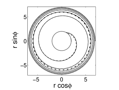
Figure 1: Comparison of our method(solid line) with EOB (dashed line, the data are calculated by Dr. Bernuzzi). Left panel: Transition from quasi-circular inspiral orbit to plunge from $r_{0}=7M$ and $\nu=0.01$. The dashed-dotted line circle is the ISCO at $r_{\text{ISCO}}=6M$ and the dotted circle the horizon of black hole; Right panel: Orbital frequency $\Omega_{\phi}$ versus coordinate time.

Furthermore, to validate our result, we check the “convergence” of the $l=m=2$ waveform modulus while $\nu\rightarrow 0$. The result is displayed in Fig. 2 and can clearly dedicate that the waveform we calculated has a good convergence. We think that this good converging trend, together with the good consistency in Fig. 1 gives a support to our theoretical idea which combines EOB dynamics with the Teukolsky perturbation method in the intermediate mass-ratio inspiral and plunge.

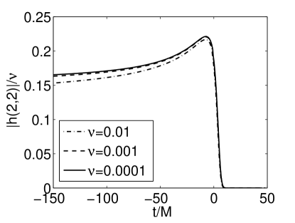
Figure 2: “Convergence” of the waveform when $\nu\rightarrow 0$ for $a=0$. The values of $\nu$ are $0.01,~{}0.001,~{}0.0001$. $t=0$ is time for the maximum of the waveform modulus and spatial position is the light ring at $r=3M$ for each value of $\nu$.

Now, as an application, we show the orbits of the small object inspiralling into Kerr black holes with different spin: $a=-0.9,~{}0.7$. We use the full EOB dynamics equations (19-22) without the $\nu\rightarrow 0$ approximation. This makes us can contain the conservative mass-ratio corrections. When $a\neq 0,~{}\nu\neq 0$, it is no possible to write out an analytical expression for the angular momentum. So we use Brent’s algorithmPress to search $L_{z}$ numerically with a relative error less than $10^{-13}$. For the Kerr black holes, because of the so-called frame-dragging effect, the radius of ISCO is smaller($a>0$) or bigger($a<0$) than the Schwarzschild case. For example, the extreme Kerr black hole, $a=\pm 1$, the ISCO locates at $r=1M$ and $r=9M$, respectively. And for $a=0.7,~{}-0.9$, $r_{\text{ISCO}}=3.39313,~{}8.71735$, respectively.

For this reason, when $a<0$ (retrograde orbit), the small body plunges faster into the black hole. At the same time, when $a>0$ (prograde orbit), the small body spirals more cycles before plunge. These phenomena are clearly displayed in Fig.3.

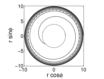
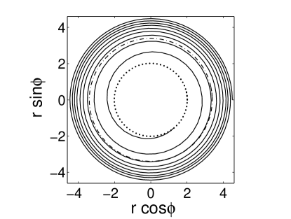
Figure 3: Inspiralling and plunge of a small body into a Kerr black hole with mass ratio $0.01$. The dashed line represents ISCO and dotted line the light ring. Left panel: retrograde orbit $a=-0.9$ beginning at $r=10M$; right panel: retrograde orbit $a=0.7$ beginning at $r=3.5M$.

In addition the waveforms are modified by different values of spin of Kerr black holes. As an example, we show the waveforms of $a=-0.9,~{}0.7$ cases in Figure 4. After passing the light ring, based on the analysis in Ref.Bernuzzi2 , the merge actually has started and gone into ringdown phase, the energy flux and waveform cannot be calculated by the frequency-domain method but can be connected by a quasi-normal mode or time-domain Teukolsky solution. For this reason, we stop the evolution just after the small object passing the light ring.

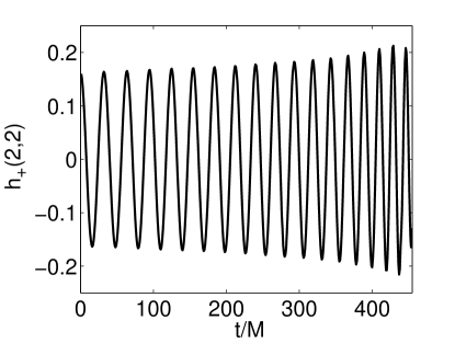
Figure 4: GW signal shown through the $l=m=2$ mode of + polarization corresponding to the dynamics depicted in Fig.3. The left panel is the retrograde orbit $a=-0.9$ and the right one retrograde orbit $a=0.7$.

V Conclusions and discussion

Previous works on IMRI dynamics through the EOB method are based on approximated analytical waveforms. We propose an alternative method to set the back reaction term for the EOB dynamics via numerically calculated energy flux directly. We have presented our numerical results based on the EOB dynamics and the frequency-domain Teukolsky flux in this paper. This is the first try to use the frequecy-domain Teukolsky frame in the plunge phase of IMRIs by the help of the EOB dynamics. Our results are consistent to the previous results using the analytical energy fluxes of post-Newtonian approximation.

And the results shown here are reasonable. By comparing with the full EOB evolution in deformed Schwarzschild space-time, a quite good coincidence before ISCO gives a support for applying the Teukolsky equation up to mass-ratio $0.01$. After ISCO, the plunge stage, a small difference comes out due to two different energy fluxes used.

Since there are few results of post-Newtonian waveforms on elliptic, and even non-equatorial orbits, it’s not easy to generalize the previous EOB dynamics works to these systems. In principle, our numerical energy-flux method is not restricted by this. The radial and polar frequencies can be obtained by evolving an “imaginary” geodesic orbit at every step. The “imaginary” geodesic orbit is the solution of Eqs.(19)-(22) but $\hat{\cal F}=0$ in (22). This solution involves ordinary differential equations with only few variables, so the computation time is negligible compared with the total evolution time. Of course, when we try to expand our method to the elliptic, and even non-equatorial orbits, the numerical cost will be more high. However, for EMRIs, there were several works which evolved generic orbits with solving the Teukolsky equation Hughes1 ; Fujita3 ; Glampedakis1 ; Glampedakis2 . For IMRIs, we can afford the numerical cost even for evolving a few tens of orbits. And more, we can generalize our analysis to generic spinning objects moving along generic elliptic, and even non-equatorial orbits. These would be our future works.

The adiabatic approximation works well in inspiral with extreme mass-ratio limit, but is violated in plunge stage. At the same time, the EOB dynamics can be used in both inspiral and plunge evolution. And then the energy fluxes also are calculated by the EOB-PN expanded waveforms usually. In this traditional method, the EOB fluxes are based on the post-Newtonian approximation, and losses accuracy in the high relativistic region. What we do in this paper is, in the EOB dynamics frame, use the Teukolsky-based energy fluxes and waveforms to replace the EOB ones. In other words, we adopt the frequency-domain Teukolsky-based energy fluxes and waveforms but abandon the adiabatic approximation; we employ the EOB dynamics to evolve the binary systems but do not use the EOB energy fluxes for back reaction.

This EOB plus Teukolsky frame we develop in this work can provide an alternative way to research the gravitational waves from IMRIs. The dynamical evolution and waveforms for several different spinning black holes are given in the above sections. But more detailed analysis about this EOB plus Teukolsky frame should be done farther in future, when more interesting results can be obtained.

References

- (1) D. A. Brown, J. Brink, H. Fang, J.R. Gair, C. Li, G. Lovelace, I. Mandel, and K.S. Thorne, Phys. Rev. Lett. 99, 201102 (2007).
- (2) C.O. Lousto, and Y. Zlochower, Phys. Rev. Lett. 106, 041101 (2011).
- (3) T. Regge, and J. Wheeler, Phys. Rev. 108, 1063 (1957).
- (4) F.J. Zerilli, Phys. Rev. D 2, 2141 (1970).
- (5) S.A. Teukolsky, Astrophy. J. 185, 635 (1973)
- (6) S.A. Teukolsky, and W.H. Press, Astrophy. J. 193, 443 (1974).
- (7) E. Poisson, Phys. Rev. D 47, 1497 (1993)
- (8) C. Cutler, D. Kennefick, and E. Poisson, Phys. Rev. D 50, 3816 (1994).
- (9) M. Shibata, Phys. Rev. D 50, 6297 (1994).
- (10) S.A. Hughes, Phys. Rev. D 61, 084004 (2000)
- (11) S.A. Hughes, Phys. Rev. D 64, 064004 (2001)
- (12) K. Glampedakis and D. Kennefick, Phys. Rev. D 66, 044002 (2002).
- (13) S. A. Hughes, S. Drasco, E.E. Flanagan, and J. Franklin, Phys. Rev. Lett. 94, 221101 (2005).
- (14) S. Drasco and S. A. Hughes, Phys. Rev. D 73, 024027 (2006).
- (15) T. Hinderer and É.É. Flanagan, Phys. Rev. D 78, 064028 (2008).
- (16) R. Fujita, W. Hikida and H. Tagoshi, Prog. Theor. Phys. 121, 843 (2009).
- (17) A. Buonanno, and T. Damour, Phys. Rev. D 59, 084006 (1999).
- (18) A. Buonanno, and T. Damour, Phys. Rev. D 62, 064015 (2000).
- (19) T. Damour, P. Jaranowski, and G. Schafer, Phys. Rev. D 62, 084011 (2000).
- (20) T. Damour, Phys. Rev. D 64, 124013 (2001).
- (21) A. Buonanno, Y. Chen, and T. Damour, Phys. Rev. D 74, 104005 (2006).
- (22) T. Damour, and A. Nagar, arXiv:0906.1769.
- (23) Y. Pan, A. Buonanno, R. Fujita, E. Racine, and H. Tagoshi, Phys. Rev. D 83, 064003 (2011)
- (24) A. Buonanno, Y. Pan, J.G. Baker, J. Centrella, B.J. Kelly, S.T. McWilliams, and J.R. van Meter, Phys. Rev. D 76, 104049 (2007).
- (25) T. Damour, A. Nagar, Phys. Rev. D 77, 024043 (2008).
- (26) T. Damour, A. Nagar, E.N. Dorband, D. Pollney, and L. Rezzolla, Phys. Rev. D 77, 084017 (2008).
- (27) T. Damour, A. Nagar, M. Hannam, S. Husa, and B. Brugmann, Phys. Rev. D 78, 044039 (2008).
- (28) M. Boyle, A. Buonanno, L.E. Kidder, A.H. Mroué, Y. Pan, H.P. Pfeiffer, and M.A. Scheel, Phys. Rev. D 78, 104020 (2008).
- (29) A. Buonanno, Y. Pan, H.P. Pfeiffer, M.A. Scheel, L.T. Buchman, and L.E. Kidder, Phys. Rev. D 79, 124028 (2009).
- (30) T. Damour, A. Nagar, Phys. Rev. D 79, 081503 (2009).
- (31) Y. Pan, A. Buonanno, L.T. Buchman, T. Chu, L.E. Kidder, H.P. Pfeiffer, and M.A. Scheel, Phys. Rev. D 81, 084041 (2010)
- (32) E. Barausse, and A. Buonanno, Phys. Rev. D 81, 084024 (2010).
- (33) A. Nagar, T. Damour and A. Tartaglia, Classical Quantum Gravity 24, S109 (2007).
- (34) S. Bernuzzi and A. Nagar, Phys. Rev. D 81, 084056 (2010).
- (35) S. Bernuzzi, A. Nagar and Anil Zenğinoglu, Phys. Rev. D83, 064010 (2011).
- (36) N. Yunes, A. Buonanno, S.A. Hughes, M. Coleman Miller, and Y. Pan, Phys. Rev. Lett. 104, 091102 (2010).
- (37) N. Yunes, A. Buonanno, S.A. Hughes, Y. Pan, E. Barausse, M.C. Miller, and W. Throwe, Phys. Rev. D83, 044044 (2011).
- (38) C.O. Lousto, H. Nakano, Y. Zlochower, and M. Campanelli, Phys. Rev. Lett. 104, 211101 (2010).
- (39) C.O. Lousto, H. Nakano, Y. Zlochower, and M. Campanelli, Phys.Rev.D 82, 104057 (2010).
- (40) T. Damour, and A. Nagar, Phys. Rev. D 76, 064028 (2007).
- (41) L. Rezzolla, E. Barausse, E. Nils Dorband, D. Pollney, C. Reisswig, J. Seiler, and S. Husa, Phys. Rev. D 78, 044002 (2008).
- (42) E. Barausse and L. Rezzolla, Astrophys. J. 704 L40 (2009).
- (43) T. Damour, B.R. Iyer and A. Nagar, Phys. Rev. D 79, 064004 (2009).
- (44) M. Sasaki and T. Nakamura, Prog. Theo. Phys, 67, 1788, 1982.
- (45) R. Fujita and H. Tagoshi, Prog.Theor.Phys. 112, 415 (2004).
- (46) R. Fujita and H. Tagoshi, Prog.Theor.Phys. 113, 1165 (2005).
- (47) S. R. Dolan, Class. Quant. Grav. 25, 235002 (2008).
- (48) S. A. Hughes, Phys. Rev. D 78, 109902(E) (2008).
- (49) W.-B. Han, Phys. Rev. D 82, 084013 (2010).
- (50) S. Mano, H. Suzuki and E. Takasugi, Prog. Theor. Phys. 98, 829 (1997).
- (51) M. Sasaki and H. Tagoshi, Living Rev. Relativity 6, 6 (2003).
- (52) R. Fujita and B.R. Iyer, Phys. Rev. D82, 044051 (2010).
- (53) W.H. Press, S.A. Teukolsky, W.T. Vetterling and B.P. Flannery, Numerical Recipes (Cambridge University Press, Cambridge, 1992).
- (54) K. Glampedakis, Class. Quant. Grav. 22, S605 (2005).