Outage Constrained Robust Transmit Optimization for Multiuser MISO Downlinks: Tractable Approximations by Conic Optimization

Abstract

In this paper we consider a probabilistic signal-to-interference-and-noise ratio (SINR) constrained problem for transmit beamforming design in the presence of imperfect channel state information (CSI), under a multiuser multiple-input single-output (MISO) downlink scenario. In particular, we deal with outage-based quality-of-service constraints, where the probability of each user’s SINR not satisfying a service requirement must not fall below a given outage probability specification. The study of solution approaches to the probabilistic SINR constrained problem is important because CSI errors are often present in practical systems and they may cause substantial SINR outages if not handled properly. However, a major technical challenge is how to process the probabilistic SINR constraints. To tackle this, we propose a novel relaxation-restriction (RAR) approach, which consists of two key ingredients— semidefinite relaxation (SDR), and analytic tools for conservatively approximating probabilistic constraints. The underlying goal is to establish approximate probabilistic SINR constrained formulations in the form of convex conic optimization problems, so that they can be readily implemented by available solvers. Using either an intuitive worst-case argument or specialized probabilistic results, we develop various conservative approximation schemes for processing probabilistic constraints with quadratic uncertainties. Consequently, we obtain several RAR alternatives for handling the probabilistic SINR constrained problem. Our techniques apply to both complex Gaussian CSI errors and i.i.d. bounded CSI errors with unknown distribution. Moreover, results obtained from our extensive simulations show that the proposed RAR methods significantly improve upon existing ones, both in terms of solution quality and computational complexity.

I Introduction

In multi-antenna multiuser downlinks, linear transmit beamforming has been recognized as an important technique, capable of leveraging quality of service (QoS) and increasing limits on the number of users served; see, e.g., the review article [3] and the references therein. Transmit beamforming design approaches developed in this context have not only been proven to offer efficient and flexible solutions for QoS optimization and interference management in standard downlinks, but have also been modified or generalized to deal with designs arising from frontier scenarios, such as relay networks [3], cognitive radios [4], and multicell coordinated downlinks [5, 6, 7].

In transmit beamforming, a very representative problem setting is the unicast multi-input single-output (MISO) downlink scenario, wherein a multi-antenna base station simultaneously transmits data streams to a number of single-antenna users, each stream for a designated user, by carefully directing transmit beams to the users. The problem of interest is to provide a signal-to-interference-and-noise ratio (SINR) constrained design formulation, in which transmit beamformers for the users are sought, so that each user is served with a QoS, characterized by the SINR, no less than a prescribed requirement, and that the transmit power is minimized. The SINR constrained problem is a meaningful and frequently used design formulation in practice, and essentially the same problem formulation can be seen in other works, such as those in the aforementioned frontier scenarios [6, 8, 9]. It is also a fundamentally intriguing problem. There are three parallel solution approaches to the problem, namely, uplink-downlink duality [10, 11], semidefinite relaxation (SDR) [5, 12], and the second-order cone programming (SOCP) formulation [13]. Each of those approaches is elegant, offering different implications both in theory and in practical implementations. They also serve as stepping stones for more advanced designs, such as those under imperfect channel state information (CSI) effects.

The SINR constrained problem, like many other transmit optimization problems, is based on the assumption that the downlink CSI is perfectly available at the base station. Unfortunately, such an assumption generally does not hold in practice [14]. In the time division duplex (TDD) setting, where there is a reciprocity between the uplink and downlink channels, the downlink CSI is typically acquired by uplink channel estimation from training data. Channel estimation errors, which are caused by noise and a limited amount of training data, result in CSI errors in this setting. In the frequency division duplex (FDD) setting, CSI acquisition is often achieved by CSI feedback with limited rates. As a result, quantization errors arising from the limited feedback lead to imperfect CSI. In addition, CSI may become somewhat outdated if the user mobility speed happens to be faster than the CSI update speed. If one uses the corrupt CSI directly to design the transmit beamformers, then the users may experience severe SINR outages and not be able to receive their anticipated QoS levels.

Recently, there has been much attention on transmit beamforming designs that are robust against CSI errors. In particular, it is of significant interest to consider “safe” SINR constrained formulations under various CSI error models, where users’ SINR requirements must be satisfied even with the worst possible CSI errors, or, alternatively, with high probability. One commonly considered formulation at present is the worst-case SINR constrained problem, in which the CSI errors are assumed to lie in a bounded set (known as the uncertainty set). This worst-case robust problem appears to be a hard (nonconvex) problem, since the worst-case SINR constraints are semi-infinite and indefinite quadratic. Several concurrent approximation schemes have been proposed to tackle the worst-case robust problem; notable works include the conservative SOCP formulation [15], the robust MMSE formulation [16, 17], and SDR [18]. The beauty of these works lies in the careful combination of robust optimization results [19] and problem formulations, leading to convex and tractable design solutions.

Another safe formulation, which is the focus of this paper, is the probabilistic, or outage-based, SINR constrained problem. In this formulation, we assume a random CSI error model, such as the popular complex Gaussian model, and the SINR outage probability of each user must be kept below a given specification. Unfortunately, while the worst-case SINR constrained problem is considered hard to solve already, this is even more so with the probabilistic SINR constrained problem— Probabilistic SINR constraints generally have no closed form expressions and are unlikely to be easily handled in an exact way. Thus, one has to resort to approximate design solutions. To date, there are very few works on the probabilistic SINR constrained problem under the unicast downlink scenario. In [20], the authors fix the transmit beam directions as zero forcing and then deal with a probabilistic power control problem. In [21], a conservative SOCP formulation is developed using some advanced results in chance constrained optimization [22, 23]. A similar approach is presented in [24], where the robust MMSE formulation is considered.

In this paper we propose several convex optimization solutions for approximating the probabilistic SINR constrained problem. Our approach is based on a relaxation-restriction (RAR) methodology. Specifically, in the relaxation step, we employ SDR to linearize the quadratic terms in the SINR expression. However, this step alone does not lead to an efficiently solvable formulation, because the probabilistic constraints imposed on the linearized SINR expressions are still nonconvex. We circumvent this problem in the restriction step, where we first derive various analytic upper bounds on the violation probability (i.e., the probability that the constraints on the linearized SINR expressions are violated). Such upper bounds serve as sufficient conditions for the probabilistic constraints to hold, hence the term “restriction”. Next, we show that our derived bounds are efficiently computable, which, together with the results from the relaxation step, leads to efficiently solvable approximations of the original probabilistic SINR constrained beamforming problem. It should be noted that the above restriction approach has many advantages. First, it allows one to generate feasible solutions to the probabilistic constraints, even when there is no closed form expression for the violation probability, or when the closed form expression is not efficiently computable. Secondly, while it may be difficult to derive closed form expressions for the violation probability, it is usually much easier to derive upper bounds on it, thanks to the many powerful techniques from the probability theory literature. Thirdly, there is usually more than one way to derive upper bounds on the violation probability, and this offers the possibility of trading approximation performance with computational complexity. These advantages will become clear in our subsequent exposition.

The rest of this paper is organized as follows. The problem statement of the outage-based SINR constrained robust beamforming design problem is given in Section II. The idea of the proposed RAR method is introduced in Section III. In Sections IV and V, various RAR formulations for complex Gaussian CSI errors are developed using either robust optimization or probabilistic techniques. An RAR formulation for i.i.d. bounded CSI errors is also presented in Section V. Simulation results are then presented in Section VI, and conclusions are drawn in Section VII.

Notations: We use boldfaced lowercase letters, e.g., ${\bm{a}}$, to represent vectors and uppercase letters, e.g., ${\bm{A}}$, to represent matrices. The notations $\mathbb{R}^{n}$, ${\mathbb{C}}^{n}$, $\mathbb{S}^{n}$, and $\mathbb{H}^{n}$ stand for the sets of $n$-dimensional real vectors, complex vectors, real symmetric matrices and complex Hermitian matrices, respectively. The superscripts ‘$T$’ and ‘$H$’ represent the transpose and (Hermitian) conjugate transpose, respectively. ${\bm{A}}\succeq{\bm{0}}$ means that the matrix ${\bm{A}}$ is positive semidefinite. ${\rm Tr}({\bm{A}})$ and $\lambda_{\max}({\bm{A}})$ denote the trace and maximum eigenvalue of ${\bm{A}}$, respectively. ${\rm vec}({\bm{A}})$ stands for the vector obtained by stacking the column vectors of ${\bm{A}}$. $[{\bm{a}}]_{i}$ and $[{\bm{A}}]_{ij}$ (or simply $a_{i}$ and $A_{ij}$) stand for the $i$th entry of ${\bm{a}}$ and $(i,j)$th entry of ${\bm{A}}$, respectively. For a complex ${\bm{A}}$, we denote by ${\rm Re}\{{\bm{A}}\}$ and ${\rm Im}\{{\bm{A}}\}$ its real and imaginary parts, respectively. ${\bm{I}}_{n}$ denotes the $n\times n$ identity matrix. Given scalars $a_{1},\ldots,a_{n}$, we use ${\rm Diag}(a_{1},\ldots,a_{n})$ to denote the $n\times n$ diagonal matrix whose $i$th diagonal entry is $a_{i}$. $\|\cdot\|$ and $\|\cdot\|_{F}$ represent the vector Euclidean norm and matrix Frobenius norm, respectively. ${\mathbb{E}}\{\cdot\}$, ${\rm Prob}\{\cdot\}$, and $\exp(\cdot)$ denote the statistical expectation, probability function and exponential function, respectively. We write ${\bm{x}}\sim\mathcal{CN}(\bm{\mu},{\bm{C}})$ if ${\bm{x}}-\bm{\mu}$ is a circular symmetric complex Gaussian random vector with covariance matrix ${\bm{C}}\succeq{\bm{0}}$.

II Problem Formulation

We focus on a downlink multiuser MISO scenario, in which the base station, or the transmitter, sends parallel data streams to multiple users over the same channel. The transmission is unicast; i.e., each data stream is exclusively for one user. The base station is equipped with $N_{t}$ transmit antennae and the signaling strategy is transmit beamforming. Let ${\bm{x}}(t)\in\mathbb{C}^{N_{t}}$ denote the multi-antenna transmit signal vector of the base station at time $t$. We have the following transmit signal model:

$${\bm{x}}(t)=\sum_{k=1}^{K}{\bm{w}}_{k}s_{k}(t),$$ (1)

where ${\bm{w}}_{k}\in\mathbb{C}^{N_{t}}$ is the transmit beamforming vector for user $k$, $K$ is the number of users, and $s_{k}(t)$ is the user-$k$ data stream, which is assumed to have zero mean and unit power (i.e., $\mathbb{E}\{|s_{k}(t)|^{2}\}=1$). It is also assumed that $s_{k}(t)$ is statistically independent of one another. For user $i$, the received signal can be modeled as

$$y_{i}(t)={\bm{h}}_{i}^{H}{\bm{x}}(t)+n_{i}(t),$$ (2)

where ${\bm{h}}_{i}\in\mathbb{C}^{N_{t}}$ is the channel from the base station to user $i$, and $n_{i}(t)$ is an additive noise, which is assumed to have zero mean and variance $\sigma_{i}^{2}>0$.

A common assumption in transmit beamforming is that the base station has perfect knowledge of ${\bm{h}}_{1},\ldots,{\bm{h}}_{K}$; i.e., the so-called perfect CSI setting. However, as discussed in detail in the Introduction, the base station may not have perfect CSI in general. In this work, the CSI is modeled as follows:

$${\bm{h}}_{i}=\bar{{\bm{h}}}_{i}+{\bm{e}}_{i},\qquad i=1,\ldots,K,$$

where ${\bm{h}}_{i}\in\mathbb{C}^{N_{t}}$ is the actual channel, $\bar{{\bm{h}}}_{i}\in\mathbb{C}^{N_{t}}$ is the presumed channel at the base station (also called the imperfect CSI), and ${\bm{e}}_{i}\in\mathbb{C}^{N_{t}}$ is the respective error that is assumed to be random. Our development will concentrate mainly on complex Gaussian CSI errors, which is a commonly adopted model. Specifically, we assume that

$${\bm{e}}_{i}\sim\mathcal{CN}(\bm{0},{\bm{C}}_{i})$$

for some known error covariance ${\bm{C}}_{i}\succeq\bm{0}$, $i=1,\ldots,K$.

The goal here is to design beamforming vectors ${\bm{w}}_{1},\ldots,{\bm{w}}_{K}$ such that the QoS of each user satisfies a prescribed set of requirements under imperfect CSI, while using the least possible amount of transmit power in doing so. To put this into context, let us consider users’ SINRs. Under the model in (1)-(2) and the associated assumptions, the SINR of user $i$ is

$$\textsf{SINR}_{i}=\frac{|{\bm{h}}^{H}_{i}{\bm{w}}_{i}|^{2}}{\sum_{k\neq i}|{\bm{h}}^{H}_{i}{\bm{w}}_{k}|^{2}+\sigma_{i}^{2}}.$$

To accommodate imperfect CSI knowledge at the base station, which causes uncertainties in the actual SINRs, we consider the following robust beamforming design problem:

Probabilistic SINR constrained problem:  Given minimum SINR requirements $\gamma_{1},\ldots,\gamma_{K}>0$ and maximum tolerable outage probabilities $\rho_{1},\ldots,\rho_{K}\in(0,1]$, solve $\displaystyle\min_{{\bm{w}}_{1},\ldots,{\bm{w}}_{K}\in\mathbb{C}^{N_{t}}}$ $\displaystyle~{}\sum_{i=1}^{K}\|{\bm{w}}_{i}\|^{2}$ (3a) $\displaystyle{\rm s.t.}$ $\displaystyle~{}{\rm Prob}_{{\bm{h}}_{i}\sim\mathcal{CN}(\bar{{\bm{h}}}_{i},{\bm{C}}_{i})}\left\{{\sf SINR}_{i}\geq\gamma_{i}\right\}\geq 1-\rho_{i},\quad i=1,\ldots,K.$ (3b)

Formulation (3) is an instance of the so-called chance constrained optimization problem due to the presence of the probabilistic constraints (3b), and it will be the main focus of this paper. In (3), the design parameters $\rho_{i}$’s govern service fidelity, making sure that each user, say, user $i$, is served with an SINR no less than $\gamma_{i}$ at least $(1-\rho_{i})\times 100\%$ of the time. In fact, the simulation results in Section VI will demonstrate that a “non-robust design”; i.e., designing the beamformers by running the perfect-CSI-based SINR constrained problem with actual channels ${{\bm{h}}}_{i}$ substituted by the presumed channels $\bar{{\bm{h}}}_{i}$, can suffer from serious SINR outage. Moreover, it should be noted that there is a tradeoff between service fidelity and design conservatism. On one hand, it is desirable to request higher service fidelity by using small values with $\rho_{i}$’s. On the other hand, the design in (3) would become more conservative as $\rho_{i}$’s decrease. In particular, for very small $\rho_{i}$’s, one may end up with design solutions that have unacceptably large transmit power, or there may be no feasible solution to (3).

Although the probabilistic SINR constrained problem in (3) is a meaningful design criterion, it is a very hard problem. The main difficulty is that the probability functions in (3b) do not yield simple closed form expressions for the considered CSI error distribution models. Thus, one may only resort to approximation methods. In the next section we will describe our proposed approximation approach.

III The Relaxation-Restriction Approach

To handle the main problem (3), we propose a novel relaxation-restriction (RAR) approach. RAR-based methods feature the use of convex optimization techniques to approximate problem (3). Hence, they can be efficiently implemented by available convex optimization software.

III-A Relaxation Step

Let us first elaborate on the first step of RAR— relaxation. The motivation is that for each $i$, the inequality ${\sf SINR}_{i}\geq\gamma_{i}$ is nonconvex in ${\bm{w}}_{1},\ldots,{\bm{w}}_{K}$; specifically, it is indefinite quadratic. We handle this issue by semidefinite relaxation (SDR) [3, 25]. To illustrate SDR for the probabilistic SINR constrained problem, we note that problem (3) can be equivalently represented by

$$\min_{{\bm{W}}_{1},\ldots,{\bm{W}}_{K}\in\mathbb{H}^{N_{t}}} ~{}\sum_{i=1}^{K}{\rm Tr}({\bm{W}}_{i})$$ (4a)

$${\rm s.t.} ~{}{\rm Prob}\left\{(\bar{{\bm{h}}}_{i}+{\bm{e}}_{i})^{H}\left(\frac{1}{\gamma_{i}}{\bm{W}}_{i}-\sum_{k\neq i}{\bm{W}}_{k}\right)(\bar{{\bm{h}}}_{i}+{\bm{e}}_{i})\geq\sigma_{i}^{2}\right\}\geq 1-\rho_{i},\quad i=1,\ldots,K,$$ (4b)

$$~{}{\bm{W}}_{1},\ldots,{\bm{W}}_{K}\succeq\bm{0},$$ (4c)

$$~{}{\rm rank}({\bm{W}}_{i})=1,\quad i=1,\ldots,K,$$ (4d)

where the connection between (3) and (4) lies in the feasible point equivalence

$${\bm{W}}_{i}={\bm{w}}_{i}{\bm{w}}_{i}^{H},\quad i=1,\ldots,K.$$

The SDR of (4) works by removing the nonconvex rank-one constraints on ${\bm{W}}_{i}$; i.e., to consider the relaxed problem

$$\min_{{\bm{W}}_{1},\ldots,{\bm{W}}_{K}\in\mathbb{H}^{N_{t}}} ~{}\sum_{i=1}^{K}{\rm Tr}({\bm{W}}_{i})$$ (5a)

$${\rm s.t.} ~{}{\rm Prob}\left\{(\bar{{\bm{h}}}_{i}+{\bm{e}}_{i})^{H}\left(\frac{1}{\gamma_{i}}{\bm{W}}_{i}-\sum_{k\neq i}{\bm{W}}_{k}\right)(\bar{{\bm{h}}}_{i}+{\bm{e}}_{i})\geq\sigma_{i}^{2}\right\}\geq 1-\rho_{i},\quad i=1,\ldots,K,$$ (5b)

$$~{}{\bm{W}}_{1},\ldots,{\bm{W}}_{K}\succeq\bm{0}.$$ (5c)

The merit of this relaxation is that the inequalities inside the probability functions in (5b) are linear in ${\bm{W}}_{1},\ldots,{\bm{W}}_{K}$, which makes the probabilistic constraints in (5b) more manageable. An issue that comes with SDR is the solution rank— the removal of ${\rm rank}({\bm{W}}_{i})=1$ means that the solution $({\bm{W}}_{1},\ldots,{\bm{W}}_{K})$ to problem (5) may have rank higher than one. We shall come back to this issue after presenting the restriction step.

III-B An Information Theoretic Interpretation of the Relaxation Step

The SDR problem (5) has an alternative interpretation from an information-theoretic point of view. Here, we briefly describe this interpretation and the resulting implications before moving to the restriction step of RAR. Consider a general transmission model:

$${\bm{x}}(t)=\sum_{i=1}^{K}{\bm{x}}_{i}(t),$$

where ${\bm{x}}_{i}(t)\in\mathbb{C}^{N_{t}}$ is the transmit signal intended for user $i$. Note that in contrast to the original transmission model in (1), where we fix the transmit scheme as beamforming by setting ${\bm{x}}_{i}(t)={\bm{w}}_{i}s_{i}(t)$, here we do not assume any specific transmit structure. As a slight abuse of notations, let ${\bm{W}}_{i}=\mathbb{E}\{{\bm{x}}_{i}(t){\bm{x}}_{i}^{H}(t)\}$ be the transmit covariance corresponding to user $i$. From an information-theoretic perspective, the achievable rate of user $i$ may be formulated as

$${\sf R}_{i}=\log_{2}\left(1+\frac{{\bm{h}}_{i}^{H}{\bm{W}}_{i}{\bm{h}}_{i}}{\sum_{k\neq i}{\bm{h}}_{i}^{H}{\bm{W}}_{k}{\bm{h}}_{i}+\sigma_{i}^{2}}\right),$$ (6)

where the rates in (6), in bits per channel use, are achieved when ${\bm{x}}_{i}(t)$ are Gaussian distributed (i.e., Gaussian codebook). One can easily verify that the SDR problem (5) is precisely the following rate optimization problem:

$$\min_{{\bm{W}}_{1},\ldots,{\bm{W}}_{K}\in\mathbb{H}^{N_{t}}} ~{}\sum_{i=1}^{K}{\rm Tr}({\bm{W}}_{i})$$ (7a)

$${\rm s.t.} ~{}{\rm Prob}_{{\bm{h}}\sim\mathcal{CN}(\bar{{\bm{h}}},{\bm{C}}_{i})}\left\{{\sf R}_{i}\geq\log_{2}(1+\gamma_{i})\right\}\geq 1-\rho_{i},\quad i=1,\ldots,K,$$ (7b)

$$~{}{\bm{W}}_{1},\ldots,{\bm{W}}_{K}\succeq\bm{0}.$$ (7c)

Specifically, the SDR equivalent (7) is a total power minimization problem that aims to ensure that each user is served with a minimal rate of $\log_{2}(1+\gamma_{i})$ bits per channel use, with an outage probability no greater than $\rho_{i}$.

With this interpretation of the SDR, we can deduce an interesting implication: If the SDR solution $({\bm{W}}_{1},\ldots,{\bm{W}}_{K})$ to (5) does not yield a rank-one structure, then an alternative to transmit beamforming is to find another practical physical-layer scheme— e.g., a space-time code with appropriate precoding— to adapt the transmit structures stipulated by the transmit covariances $({\bm{W}}_{1},\ldots,{\bm{W}}_{K})$. While our main interest in this paper is still in transmit beamforming, it is worthwhile to keep such a parallel possibility in mind, since it eliminates the need for rank-one transmit covariances.

III-C Restriction Step

Let us continue to illustrate the second step of RAR— restriction. The relaxation step alone does not provide a convex approximation of the main problem (3). The SDR probabilistic constraints (5b) remain intractable, although they appear to be relatively easier to handle than the original counterparts in (3b). The restriction step aims to find a convex approximation of (5b), in a restrictive or conservative sense. More precisely, in the context of the probabilistic SINR constrained problem, the restriction step entails finding a solution to the following:

Challenge 1:  Consider the following chance constraint: $${\rm Prob}\{{\bm{e}}^{H}{\bm{Q}}{\bm{e}}+2{\rm Re}\{{\bm{e}}^{H}{\bm{r}}\}+s\geq 0\}\geq 1-\rho,$$ (8) where ${\bm{e}}\in\mathbb{C}^{n}$ is a standard complex Gaussian vector (i.e., ${\bm{e}}\sim\mathcal{CN}(\bm{0},{\bm{I}}_{n})$), the 3-tuple $({\bm{Q}},{\bm{r}},s)\in\mathbb{H}^{n}\times\mathbb{C}^{n}\times\mathbb{R}$ is a set of (deterministic) optimization variables, and $\rho\in(0,1]$ is fixed. Find an efficiently computable convex restriction of (8); i.e., find an efficiently computable convex set $\mathcal{S}\subset\mathbb{H}^{n}\times\mathbb{C}^{n}\times\mathbb{R}\times\mathbb{C}^{\ell}$ such that whenever $({\bm{Q}},{\bm{r}},s,{\bm{t}})\in\mathcal{S}$, the 3-tuple $({\bm{Q}},{\bm{r}},s)\in\mathbb{H}^{n}\times\mathbb{C}^{n}\times\mathbb{R}$ is feasible for (8).

Note that in the construction of the convex set $\mathcal{S}$, we are allowed to include an extra optimization variable ${\bm{t}}\in\mathbb{C}^{\ell}$, in addition to the original optimization variables $({\bm{Q}},{\bm{r}},s)\in\mathbb{H}^{n}\times\mathbb{C}^{n}\times\mathbb{R}$. Although the precise role of ${\bm{t}}$ will depend on how the set $\mathcal{S}$ is formulated, it suffices to think of ${\bm{t}}$ as a slack variable.

It is not hard to see that the SDR probabilistic constraints in (5b) fall in the scope of Challenge 1. Indeed, for each constraint in (5b), the following correspondence to (8) can be shown:

$${\bm{Q}}={\bm{C}}_{i}^{1/2}\left(\frac{1}{\gamma_{i}}{\bm{W}}_{i}-\sum_{k\neq i}{\bm{W}}_{k}\right){\bm{C}}_{i}^{1/2},\quad {\bm{r}}={\bm{C}}_{i}^{1/2}\left(\frac{1}{\gamma_{i}}{\bm{W}}_{i}-\sum_{k\neq i}{\bm{W}}_{k}\right)\bar{{\bm{h}}}_{i},$$ (9a)

$$s=\bar{{\bm{h}}}_{i}^{H}\left(\frac{1}{\gamma_{i}}{\bm{W}}_{i}-\sum_{k\neq i}{\bm{W}}_{k}\right)\bar{{\bm{h}}}_{i}-\sigma_{i}^{2},\quad \rho=\rho_{i}.$$ (9b)

The development of convex restriction methods plays a crucial role in RAR, and this will be our focus in subsequent sections. By replacing each probabilistic constraint in (5b) with a convex restriction, we will obtain a convex approximation of the original probabilistic SINR constrained problem. Table I summarizes all the RAR methods to be proposed in later sections. Note that each RAR method is based on a different convex restriction. Moreover, all the RAR formulations in Table I are conic problems with linear matrix inequality constraints and/or second-order cone constraints, which can be easily solved by off-the-shelf convex optimization software [26].

TABLE I: The proposed RAR formulations.

Method	RAR Formulation
Method I: Sphere bounding (for complex Gaussian CSI errors)	​​​​​ $\displaystyle\begin{array}[]{ll}{\displaystyle\min_{\begin{subarray}{c}{\bm{W}}_{i}\in\mathbb{H}^{N_{t}},t_{i}\in{\mathbb{R}},\\ i=1,\ldots,K\end{subarray}}~{}\sum_{i=1}^{K}{{\rm Tr}}({\bm{W}}_{i})}\\ ~{}~{}~{}~{}~{}~{}~{}~{}~{}~{}~{}~{}~{}{\rm s.t.}~{}\begin{bmatrix}\!\!\!\!\!\!\!{\bm{Q}}_{i}+t_{i}{\bm{I}}_{N_{t}}~{}~{}~{}~{}~{}~{}{\bm{r}}_{i}\\ ~{}~{}~{}~{}~{}{\bm{r}}_{i}^{H}~{}~{}~{}~{}~{}~{}~{}~{}s_{i}-t_{i}d^{2}_{i}\end{bmatrix}\succeq\bm{0},~{}i=1,\ldots,K,\\ ~{}~{}~{}~{}~{}~{}~{}~{}~{}~{}~{}~{}~{}~{}~{}~{}~{}~{}~{}{\bm{W}}_{1},\ldots,{\bm{W}}_{K}\succeq{\bm{0}},~{}t_{1},\ldots,t_{K}\geq 0;\end{array}$ (13) where ${\bm{Q}}_{i}$, ${\bm{r}}_{i}$ and $s_{i}$ are defined in the same way as (9), and $d_{i}=\sqrt{\Phi_{\chi^{2}_{2n}}^{-1}(1-\rho_{i})/2}$, $i=1,\ldots,K$.
Method II: Bernstein-type inequality (for complex Gaussian CSI errors)	​​​ $\displaystyle\begin{array}[]{ll}{\displaystyle\min_{\begin{subarray}{c}{\bm{W}}_{i}\in\mathbb{H}^{N_{t}},x_{i},y_{i}\in\mathbb{R},\\ i=1,\ldots,K\end{subarray}}~{}\sum_{i=1}^{K}{\rm Tr}(\bm{W}_{i})}\\ ~{}~{}~{}~{}~{}~{}~{}~{}~{}~{}~{}~{}~{}~{}~{}{\rm s.t.}~{}{\rm Tr}({\bm{Q}}_{i})-\sqrt{-2\ln(\rho_{i})}\cdot x_{i}+\ln(\rho_{i})\cdot y_{i}+s_{i}\geq 0,~{}i=1,\ldots,K,\\ \ ~{}~{}~{}~{}~{}~{}~{}~{}~{}~{}~{}~{}~{}~{}~{}~{}~{}~{}~{}~{}\left\|\begin{bmatrix}{\rm vec}({\bm{Q}}_{i})\\ \sqrt{2}{\bm{r}}_{i}\end{bmatrix}\right\|\leq x_{i},~{}i=1,\ldots,K,\\ ~{}~{}~{}~{}~{}~{}~{}~{}~{}~{}~{}~{}~{}~{}~{}~{}~{}~{}~{}~{}y_{i}{\bm{I}}_{N_{t}}+{\bm{Q}}_{i}\succeq{\bm{0}},~{}i=1,\ldots,K,\\ ~{}~{}~{}~{}~{}~{}~{}~{}~{}~{}~{}~{}~{}~{}~{}~{}~{}~{}~{}~{}y_{1},\ldots,y_{K}\geq 0,~{}{\bm{W}}_{1},\ldots,{\bm{W}}_{K}\succeq{\bm{0}};\end{array}$ (19) where ${\bm{Q}}_{i}$, ${\bm{r}}_{i}$ and $s_{i}$ are defined in the same way as (9), $i=1,\ldots,K$.
Method III: Decomposition into independent parts (for complex Gaussian CSI errors)	​​​ $\displaystyle\begin{array}[]{ll}{\displaystyle\min_{\begin{subarray}{c}{\bm{W}}_{i}\in\mathbb{H}^{N_{t}},x_{i},y_{i}\in\mathbb{R},\\ i=1,\ldots,K\end{subarray}}~{}\sum_{i=1}^{K}{{\rm Tr}}({\bm{W}}_{i})}\\ ~{}~{}~{}~{}~{}~{}~{}~{}~{}~{}~{}~{}~{}{\rm s.t.}~{}s_{i}+{\rm Tr}({\bm{Q}}_{i})\geq 2\sqrt{-\ln(\rho_{i})}\cdot(x_{i}+y_{i}),~{}i=1,\ldots,K,\\ ~{}~{}~{}~{}~{}~{}~{}~{}~{}~{}~{}~{}~{}~{}~{}~{}~{}\frac{1}{\sqrt{2}}\|{\bm{r}}_{i}\|\leq x_{i},~{}i=1,\ldots,K,\\ ~{}~{}~{}~{}~{}~{}~{}~{}~{}~{}~{}~{}~{}~{}~{}~{}~{}~{}v_{i}\left\|{\rm vec}({\bm{Q}}_{i})\right\|\leq y_{i},~{}i=1,\ldots,K,\\ ~{}~{}~{}~{}~{}~{}~{}~{}~{}~{}~{}~{}~{}~{}~{}~{}~{}~{}{\bm{W}}_{1},\ldots,{\bm{W}}_{K}\succeq{\bm{0}};\end{array}$ (25) where ${\bm{Q}}_{i}$, ${\bm{r}}_{i}$ and $s_{i}$ are defined in the same way as (9), $\bar{\theta}_{i}$ is chosen such that $\bar{\theta}_{i}+\ln(1-\bar{\theta}_{i})=\ln(\rho_{i})$, and $v_{i}=\sqrt{-\ln(\rho_{i})/\bar{\theta}_{i}^{2}}$, $i=1,\ldots,K$.
Method IV: Decomposition into independent parts (for elementwise i.i.d. and bounded CSI errors with mean 0 and variance $\sigma_{e}^{2}$, but otherwise unknown distribution)	​​​ $\displaystyle\begin{array}[]{ll}{\displaystyle\min_{\begin{subarray}{c}{\bm{W}}_{i}\in\mathbb{H}^{N_{t}},{\bm{t}}_{i}\in\mathbb{R}^{2N_{t}+1}\\ i=1,\ldots,K\end{subarray}}~{}\sum_{i=1}^{K}{\rm Tr}(\bm{W}_{i})}\\ ~{}~{}~{}~{}~{}~{}~{}~{}~{}~{}~{}~{}~{}~{}~{}{\rm s.t.}~{}s_{i}+\sigma_{e}^{2}\cdot{\rm Tr}({\bm{Q}}_{i})\geq 2\sqrt{-\ln(\rho_{i})}\cdot\sum_{\ell=0}^{2N_{t}}[{\bm{t}}_{i}]_{\ell},~{}\forall i,\\ ~{}~{}~{}~{}~{}~{}~{}~{}~{}~{}~{}~{}~{}~{}~{}~{}~{}~{}~{}~{}\sqrt{2}\|{\bm{r}}_{i}\|\leq[{\bm{t}}_{i}]_{0},~{}i=1,\ldots,K,\\ ~{}~{}~{}~{}~{}~{}~{}~{}~{}~{}~{}~{}~{}~{}~{}~{}~{}~{}~{}~{}\left(\sum_{(j,k)\in\mathcal{A}_{\ell}}v_{jk}^{2}[{\bm{Q}}_{i}]_{jk}^{2}\right)^{1/2}\leq[{\bm{t}}_{i}]_{\ell},\\ ~{}~{}~{}~{}~{}~{}~{}~{}~{}~{}~{}~{}~{}~{}~{}~{}~{}~{}~{}~{}~{}~{}~{}~{}~{}~{}~{}~{}~{}~{}~{}~{}~{}~{}~{}~{}\ell=1,\ldots,2N_{t},~{}i=1,\ldots,K,\\ ~{}~{}~{}~{}~{}~{}~{}~{}~{}~{}~{}~{}~{}~{}~{}~{}~{}~{}~{}~{}{\bm{W}}_{1},\ldots,{\bm{W}}_{K}\succeq{\bm{0}};\end{array}$ (32) where ${\bm{Q}}_{i}$, ${\bm{r}}_{i}$ and $s_{i}$ are defined in the same way as (53), $\mathcal{A}_{\ell}$ are defined in the same way as Table II, and $v_{jj}=1/\sqrt{8}$ and $v_{jk}=1$ if $j\neq k$.

The last step of RAR is to provide a feasible beamforming solution $({\bm{w}}_{1},\ldots,{\bm{w}}_{K})$ to the main problem (3) by using the RAR solution $({\bm{W}}_{1},\ldots,{\bm{W}}_{K})$. As is common in all SDR-based methods, the ${\bm{W}}_{i}$’s obtained from RAR may have rank higher than one. A standard way of tackling this issue is to apply some rank-one approximation procedure to $({\bm{W}}_{1},\ldots,{\bm{W}}_{K})$ to generate a feasible beamforming solution $({\bm{w}}_{1},\ldots,{\bm{w}}_{K})$ to (3); see [25] for a review and references. In our setting, we apply a Gaussian randomization procedure to a non-rank-one RAR solution. The procedure is provided in Algorithm 1; the spirit follows that of [27], and readers are referred to [27] for an exposition of the idea. We should point out that obtaining a feasible RAR solution does not imply that we can always generate a feasible solution to the main problem (3). This issue has also been identified before in the context of multigroup multicast beamforming with perfect CSI [27]. However, if the RAR solution happens to give rank-one ${\bm{W}}_{i}$ for all $i$, then we can simply solve the rank-one decomposition ${\bm{W}}_{i}={\bm{w}}_{i}{\bm{w}}_{i}^{H}$ and output the corresponding $({\bm{w}}_{1},\ldots,{\bm{w}}_{K})$ as the approximate beamforming solution. For such instances, it can be easily verified that $({\bm{w}}_{1},\ldots,{\bm{w}}_{K})$ is already feasible for the main problem (3). Rather surprisingly, we found that the proposed RAR methods returned rank-one solutions in almost all the simulation trials we ran. Such empirical finding provides another interesting implication when we consider the information-theoretic interpretation in the last subsection: Since the RAR methods are essentially the same as convex restrictions of the outage-based rate optimization problem in (7), the numerical observation that RAR solutions are almost always rank-one somehow hints that transmit beamforming may inherently be an optimal physical-layer scheme, at least for the outage-based unicast multiuser MISO downlink scenario considered here.

1

Given : A number of randomizations $L$, and an optimal solution $({\bm{W}}_{1}^{\star},\dots,{\bm{W}}_{K}^{\star})$ to an employed RAR formulation.

2

3for $\ell=1,\ldots,L$ do

4      generate random vectors ${\bm{w}}_{i}^{(\ell)}\sim\mathcal{CN}(\bm{0},{\bm{W}}_{i}^{\star})$, $i=1,\ldots,K$;

5      set beam directions ${\bm{u}}_{i}^{(\ell)}={{\bm{w}}_{i}^{(\ell)}}/{\|{\bm{w}}_{i}^{(\ell)}\|}$, $i=1,\ldots,K$;

6      let $p_{1}^{(\ell)},\ldots,p_{K}^{(\ell)}$ be beam powers and obtain $p_{1}^{(\ell)},\ldots,p_{K}^{(\ell)}$ as follows: substitute $\bm{W}_{i}=p_{i}{\bm{u}}_{i}^{(\ell)}({\bm{u}}_{i}^{(\ell)})^{H}$, $i=1,\ldots,K$, into the RAR problem, solve the problem with respect to $p_{1},\ldots,p_{K}\geq 0$, and set $p_{1}^{(\ell)},\ldots,p_{K}^{(\ell)}$ as its solution if the problem is feasible; also, set $P^{(\ell)}$ to be the associated optimal objective value if the problem is feasible; otherwise set $P^{(\ell)}=\infty$ ;

7     

8      end for

9     

10     $\ell^{\star}=\arg\min_{\ell=1,\ldots,L}P^{(\ell)}$.

     Output : $\hat{}{\bm{w}}_{i}^{\star}=\sqrt{p_{i}^{(\ell^{\star})}}{\bm{u}}_{i}^{(\ell^{\star})}$, $i=1,\ldots,K$, as an approximate solution to the main problem (3).

11     

Algorithm 1 Gaussian randomization procedure for RAR

As a summary to the solution approximation aspect discussed above, in most cases a simple rank-one decomposition ${\bm{W}}_{i}={\bm{w}}_{i}{\bm{w}}_{i}^{H}$ of the RAR solution suffices to produce a feasible solution $({\bm{w}}_{1},\ldots,{\bm{w}}_{K})$ to the main problem (3). The more complicated solution approximation procedure in Algorithm 1, proposed for instances where the RAR solution is not of rank one, is rarely needed in our empirical experience.

IV RAR Method I: Sphere Bounding

In this section we describe our first convex restriction method for Challenge 1. The method is based on two key ingredients. The first is the following lemma:

Lemma 1

Consider Challenge 1. Suppose that we have a set $\mathcal{B}\subset\mathbb{C}^{n}$ that satisfies

$${\rm Prob}\{\bm{e}\in\mathcal{B}\}\geq 1-\rho.$$ (33)

Then, the following implication holds:

$$\begin{array}[]{c}\bm{\delta}^{H}\bm{Q}\bm{\delta}+2{\rm Re}\{\bm{\delta}^{H}\bm{r}\}+s\geq 0,\\ \text{for all~{}}\bm{\delta}\in\mathcal{B}\end{array}\Longrightarrow\text{Eq.~{}(8) in Challenge 1 holds.}$$ (34)

The proof of Lemma 1 is simple and is given as follows. Let $p(\bm{e})$ denote the probability density function of $\bm{e}$. Suppose that (33) and the left-hand side (LHS) of (34) hold. Then, we have the following chain:

$${\rm Prob}\{\bm{e}^{H}\bm{Q}\bm{e}+2{\rm Re}\{\bm{r}^{H}\bm{e}\}+s\geq 0\} =\int_{\bm{e}^{H}\bm{Q}\bm{e}+2{\rm Re}\{\bm{r}^{H}\bm{e}\}+s\geq 0}p(\bm{e})d\bm{e}$$

$$\geq\int_{\bm{e}\in\mathcal{B}}p(\bm{e})d\bm{e}$$

$$\geq 1-\rho.$$

Hence, Eq. (8) is satisfied.

Lemma 1 suggests that we can approximate the chance constraint in (8) in a conservative (or restrictive) fashion by using the worst-case deterministic constraint on the LHS of (34). Moreover, it can be easily seen that the same idea applies to general chance constraints; i.e., the quadratic functions in (8) and (34) may be replaced by any arbitrary function. Such an insight (i.e., using worst-case deterministic constraints to approximate (general) chance constraints) have been alluded to or used in many different contexts; e.g., [28, 29] in optimization. Here, we are interested in the chance constraint in (8), which involves a quadratic function of the standard complex Gaussian vector $\bm{e}$. In our method, we choose $\mathcal{B}$ to be a spherical set; i.e.,

$$\mathcal{B}=\{\bm{\delta}\in\mathbb{C}^{n}\mid\|\bm{\delta}\|\leq d\},$$ (35)

where $d$ is the sphere radius. It can be shown that by choosing

$$d=\sqrt{\frac{\Phi_{\chi^{2}_{2n}}^{-1}(1-\rho)}{2}},$$

where $\Phi_{\chi^{2}_{m}}^{-1}(\cdot)$ is the inverse cumulative distribution function of the (central) Chi-square random variable with $m$ degrees of freedom, Eq. (33) is satisfied.

The second ingredient is the so-called $\mathcal{S}$-lemma, which enables us to turn the infinitely many constraints on the LHS of (34) into a set of tractable constraints. The $\mathcal{S}$-lemma is given as follows:

Lemma 2 ( $\mathcal{S}$-lemma [30] )

Let $f_{i}(\bm{x})=\bm{x}^{H}\bm{Q}_{i}\bm{x}+2{\rm Re}\{\bm{x}^{H}\bm{r}_{i}\}+s_{i}$ for $i=0,1$, where $\bm{x}\in\mathbb{C}^{n}$ and $(\bm{Q}_{i},\bm{r}_{i},s_{i})\in\mathbb{H}^{n}\times\mathbb{C}^{n}\times\mathbb{R}$ for $i=0,1$. Suppose that there exists an $\hat{\bm{x}}\in\mathbb{C}^{n}$ satisfying $f_{1}(\hat{\bm{x}})<0$. Then, the following statements are equivalent:

• $f_{0}(\bm{x})\geq 0$ for all $\bm{x}\in\mathbb{C}^{n}$ satisfying $f_{1}(\bm{x})\leq 0$.

• There exists a $t\geq 0$ such that

  $$\begin{bmatrix}\bm{Q}_{0}&\bm{r}_{0}\\ \bm{r}_{0}^{H}&s_{0}\end{bmatrix}+t\begin{bmatrix}\bm{Q}_{1}&\bm{r}_{1}\\ \bm{r}_{1}^{H}&s_{1}\end{bmatrix}\succeq\bm{0}.$$ (36)

By the $\mathcal{S}$-lemma, the LHS of (34), with $\mathcal{B}$ given by (35), can be equivalently represented by an LMI of the form (36), where $(\bm{Q}_{0},\bm{r}_{0},s_{0})=(\bm{Q},\bm{r},s)$ and $(\bm{Q}_{1},\bm{r}_{1},s_{1})=({\bm{I}}_{n},\bm{0},-d^{2})$. We therefore have built a convex restriction for Challenge 1. To summarize, we have the following:

Method I for Challenge 1 (Sphere bounding):  The following feasibility problem is a convex restriction of (8) in Challenge 1: Find $\displaystyle~{}~{}{\bm{Q}},{\bm{r}},s,t$ s.t. $\displaystyle~{}~{}\begin{bmatrix}\bm{Q}+t{\bm{I}}_{n}&\bm{r}\\ \bm{r}^{H}&s-td^{2}\end{bmatrix}\succeq\bm{0},$ $\displaystyle~{}~{}t\geq 0,$ where $d=\sqrt{\Phi_{\chi^{2}_{2n}}^{-1}(1-\rho)/2}$.

By first applying SDR and then Method I to the probabilistic SINR constrained problem (3), we obtain the RAR formulation (13) in Table I. Interestingly, this formulation turns out to be similar to that of the worst-case robust SDR problem considered in [18]. However, it should be noted that the prior work does not consider outage probability constraints. Moreover, we show a way of using the worst-case robust formulation to deal with the probabilistic SINR constrained problem. Finally, by incorporating the bisection scheme proposed in [21], which will be considered in our simulations in Section VI (Example 3), we will be able to further improve the performance of the sphere bounding RAR method.

V Probability Inequality Approaches

The reader may notice that the development of Method I is strongly motivated by the worst-case robust optimization paradigm. Indeed, the problem on the LHS of the implication (34) is precisely a robust feasibility problem with uncertainty set $\mathcal{B}$. By choosing $\mathcal{B}$ judiciously, it is shown that the violation probability ${\rm Prob}\{\bm{e}^{H}\bm{Q}\bm{e}+2{\rm Re}\{\bm{r}^{H}\bm{e}\}+s<0\}$ can be controlled, and the resulting robust feasibility problem is a convex restriction of (8). However, this approach has an intrinsic drawback, namely, it is difficult to define and analyze an uncertainty set $\mathcal{B}$ other than those that have very simple geometry, such as the spherical set considered in the previous section. Consequently, it is not clear whether there exist other choices of $\mathcal{B}$ that would lead to better convex restrictive approximations.

As it turns out, one can circumvent the above drawback by using analytic upper bounds on the violation probability to construct efficiently computable convex restrictions of (8). Specifically, suppose that we have an efficiently computable convex function $f(\bm{Q},\bm{r},s,\bm{t})$, where $\bm{t}$ is an extra optimization variable, such that

$${\rm Prob}\{{\bm{e}}^{H}{\bm{Q}}{\bm{e}}+2{\rm Re}\{{\bm{e}}^{H}{\bm{r}}\}+s<0\}\leq f(\bm{Q},\bm{r},s,\bm{t}).$$ (37)

Then, the constraint

$$f(\bm{Q},\bm{r},s,\bm{t})\leq\rho$$ (38)

is, by construction, a convex restriction of (8). An upshot of this approach is that there are many available techniques for constructing such upper bounds, and each of those bounds yields a convex restriction of (8). Moreover, it is known [19, Chapter 4] that under some fairly mild conditions, every convex restriction corresponds to a robust feasibility problem with a suitably defined uncertainty set. Thus, the above approach can be viewed as an enhancement of Method I, in the sense that it provides a handle on more sophisticated uncertainty sets that are difficult to construct directly.

V-A Method II: Bernstein-Type Inequality

Let us now illustrate the above approach by showing how a Bernstein-type inequality for Gaussian quadratic forms can be used to construct a convex restriction of (8). Our approach relies on the following lemma due to Bechar [31]:

Lemma 3

Let ${\bm{e}}\sim\mathcal{CN}({\bm{0}},{\bm{I}}_{n})$, ${\bm{Q}}\in\mathbb{H}^{n}$ and ${\bm{r}}\in\mathbb{C}^{n}$. Then, for any $\eta>0$, we have

$${\rm Prob}\{{\bm{e}}^{H}{\bm{Q}}{\bm{e}}+2{\rm Re}\{{\bm{e}}^{H}{\bm{r}}\}\geq T(\eta)\}\geq 1-e^{-\eta},$$ (39)

where the function $T:\mathbb{R}_{++}\rightarrow\mathbb{R}$ is defined by

$$T(\eta)={\rm Tr}({\bm{Q}})-\sqrt{2\eta}\sqrt{\|{\bm{Q}}\|_{F}^{2}+2\|{\bm{r}}\|^{2}}-\eta\lambda^{+}({\bm{Q}}),$$ (40)

with $\lambda^{+}({\bm{Q}})=\max\{\lambda_{\max}(-{\bm{Q}}),0\}$.

Lemma 3 is obtained by extending the corresponding result in [31] for quadratic forms of real-valued Gaussian random variables. The inequality in (39) is a so-called Bernstein-type inequality, which bounds the probability that the quadratic form ${\bm{e}}^{H}{\bm{Q}}{\bm{e}}+2{\rm Re}\{{\bm{e}}^{H}{\bm{r}}\}$ of complex Gaussian random variables deviates from its mean ${\rm Tr}({\bm{Q}})$.

Since $T(\eta)$ is monotonically decreasing, its inverse mapping $T^{-1}:\mathbb{R}\rightarrow\mathbb{R}_{++}$ is well defined. In particular, the Bernstein-type inequality in (39) can be expressed as

$${\rm Prob}\{{\bm{e}}^{H}{\bm{Q}}{\bm{e}}+2{\rm Re}\{{\bm{e}}^{H}{\bm{r}}\}+s\geq 0\}\geq 1-e^{-T^{-1}(-s)}.$$ (41)

As discussed in (37) and (38), the constraint $e^{-T^{-1}(-s)}\leq\rho$, or equivalently,

$${\rm Tr}({\bm{Q}})-\sqrt{-2\ln(\rho)}\sqrt{\|{\bm{Q}}\|_{F}^{2}+2\|{\bm{r}}\|^{2}}+\ln(\rho)\cdot\lambda^{+}({\bm{Q}})+s\geq 0$$ (42)

serves as a sufficient condition for achieving (8).

While it is not obvious at this stage whether (42) is convex in $({\bm{Q}},{\bm{r}},s)$ or not, a crucial observation is that (42) can be equivalently represented by the following system of convex conic inequalities:

$$~{}{\rm Tr}\left({\bm{Q}}\right)-\sqrt{-2\ln(\rho)}\cdot t_{1}+\ln(\rho)\cdot t_{2}+s\geq 0,$$ (43a)

$$~{}\sqrt{\|{\bm{Q}}\|_{F}^{2}+2\|{\bm{r}}\|^{2}}\leq t_{1},$$ (43b)

$$~{}t_{2}{\bm{I}}_{n}+{\bm{Q}}\succeq{\bm{0}},$$ (43c)

$$~{}t_{2}\geq 0,$$ (43d)

where $t_{1},t_{2}\in\mathbb{R}$ are slack variables. Therefore, formulation (43) is an efficiently computable convex restriction of (8). We now summarize the Bernstein-type inequality method as follows:

Method II for Challenge 1 (Bernstein-type inequality method):  The following feasibility problem is a convex restriction of (8) in Challenge 1: Find $\displaystyle~{}~{}{\bm{Q}},{\bm{r}},s,{\bm{t}}$ s.t. $\displaystyle~{}~{}{\rm Tr}\left({\bm{Q}}\right)-\sqrt{-2\ln(\rho)}\cdot t_{1}+\ln(\rho)\cdot t_{2}+s\geq 0,$ $\displaystyle~{}~{}\sqrt{\|{\bm{Q}}\|_{F}^{2}+2\|{\bm{r}}\|^{2}}\leq t_{1},$ $\displaystyle~{}~{}t_{2}{\bm{I}}_{n}+{\bm{Q}}\succeq{\bm{0}},$ $\displaystyle~{}~{}t_{2}\geq 0.$

Upon applying Method II to (5), we obtain the RAR formulation (19) in Table I. As can be easily seen from the formulations (13) and (19), the latter has a more complex constraint set and thus a higher computational complexity in general. However, it will be shown later that the Bernstein-type inequality method (19) exhibits better approximation performance than the sphere bounding method.

V-B Method III: Decomposition into Independent Parts

For both the sphere bounding and Bernstein-type inequality methods, the resulting convex restrictions of (8) contain linear matrix inequality constraints. As such, they could be computationally costly when the problem size is large. It turns out that one can also develop a convex restriction of (8) that contains only second-order cone constraints. The resulting formulation can thus be solved more efficiently than those developed using the sphere bounding or Bernstein-type inequality method. The idea is to first decompose the sum ${\bm{e}}^{H}{\bm{Q}}{\bm{e}}+2{\rm Re}\{{\bm{e}}^{H}{\bm{r}}\}+s$ into several parts, each of which is a sum of independent random variables. Then, one bounds the moment generating function of each of those parts and stitch the results together to obtain an analytic upper bound on the violation probability [32]. To illustrate this approach, let ${\bm{Q}}={\bm{U}}{\bm{\Lambda}}{\bm{U}}^{H}$ be the spectral decomposition of ${\bm{Q}}$, where ${\bm{\Lambda}}={\rm Diag}(\lambda_{1},\ldots,\lambda_{n})$ and $\lambda_{1},\ldots,\lambda_{n}$ are the eigenvalues of ${\bm{Q}}$. Since ${\bm{e}}\sim\mathcal{CN}({\bm{0}},{\bm{I}}_{n})$ and ${\bm{U}}^{H}$ is unitary, we have $\tilde{{\bm{e}}}={\bm{U}}^{H}{\bm{e}}\sim\mathcal{CN}({\bm{0}},{\bm{I}}_{n})$. Thus, we can write

$$\Psi={\bm{e}}^{H}{\bm{Q}}{\bm{e}}+2{\rm Re}\{{\bm{e}}^{H}{\bm{r}}\}=\tilde{{\bm{e}}}^{H}{\bm{\Lambda}}\tilde{{\bm{e}}}+2{\rm Re}\{{\bm{e}}^{H}{\bm{r}}\}=\Psi_{q}+\Psi_{l}.$$

Now, observe that both

$$\Psi_{q}=\tilde{{\bm{e}}}^{H}{\bm{\Lambda}}\tilde{{\bm{e}}}=\sum_{\ell=1}^{n}\lambda_{\ell}|e_{\ell}|^{2}\quad\mbox{and}\quad\Psi_{l}=2{\rm Re}\{{\bm{e}}^{H}{\bm{r}}\}=2\sum_{\ell=1}^{n}\left({\rm Re}\{r_{\ell}\}{\rm Re}\{e_{\ell}\}+{\rm Im}\{r_{\ell}\}{\rm Im}\{e_{\ell}\}\right)$$

are sums of independent random variables. Moreover, it can be shown that for any fixed $\bar{\theta}<1$,

$${\mathbb{E}}\left\{\exp\left(\theta(|e_{\ell}|^{2}-1)\right)\right\}=\frac{\exp(-\theta)}{1-\theta}\leq\exp\left(v^{2}\theta^{2}\right),$$

$${\mathbb{E}}\left\{\exp\left(\theta\cdot 2{\rm Re}\{e_{\ell}\}\right)\right\}={\mathbb{E}}\left\{\exp\left(\theta\cdot 2{\rm Im}\{e_{\ell}\}\right)\right\}=\exp\left(\frac{1}{2}\theta^{2}\right)\quad\mbox{for }\theta\in{\mathbb{R}},$$

where $v=\left(-\left(\bar{\theta}+\ln\left(1-\bar{\theta}\right)\right)/\bar{\theta}^{2}\right)^{1/2}<\infty$. Thus, for any $p_{1},p_{2}>0$ such that $p_{1}+p_{2}=1$, the chain of inequalities

$${\mathbb{E}}\left\{\exp(u({\rm Tr}({\bm{\Lambda}})-\Psi))\right\}= ~{}{\mathbb{E}}\left\{\exp\left(p_{1}\cdot\frac{(-u)}{p_{1}}(\Psi_{q}-{\rm Tr}({\bm{\Lambda}}))+p_{2}\cdot\frac{(-u)}{p_{2}}\Psi_{l}\right)\right\}$$

$$\leq ~{}p_{1}{\mathbb{E}}\left\{\exp\left(-\frac{u}{p_{1}}(\Psi_{q}-{\rm Tr}({\bm{\Lambda}}))\right)\right\}+p_{2}{\mathbb{E}}\left\{\exp\left(-\frac{u}{p_{2}}\Psi_{l}\right)\right\}$$ (44)

$$= ~{}p_{1}\prod_{\ell=1}^{n}{\mathbb{E}}\left\{\exp\left(-\frac{u}{p_{1}}\lambda_{\ell}(|e_{\ell}|^{2}-1)\right)\right\}$$ (45)

$$+p_{2}\prod_{\ell=1}^{n}{\mathbb{E}}\left\{\exp\left(-\frac{u}{p_{2}}2{\rm Re}\{r_{\ell}\}{\rm Re}\{e_{\ell}\}\right)\right\}{\mathbb{E}}\left\{\exp\left(-\frac{u}{p_{2}}2{\rm Im}\{r_{\ell}\}{\rm Im}\{e_{\ell}\}\right)\right\}$$

$$\leq ~{}p_{1}\exp\left(\sum_{\ell=1}^{n}v^{2}\frac{u^{2}\lambda_{\ell}^{2}}{p_{1}^{2}}\right)+p_{2}\exp\left(\sum_{\ell=1}^{n}\frac{1}{2}\left(\frac{u^{2}{\rm Re}\{r_{\ell}\}^{2}}{p_{2}^{2}}+\frac{u^{2}{\rm Im}\{r_{\ell}\}^{2}}{p_{2}^{2}}\right)\right)$$ (46)

holds whenever $-u\lambda_{\ell}/p_{1}<\bar{\theta}$ for $\ell=1,\ldots,n$, where (44) follows from Jensen’s inequality and (45) follows from the independence of the random variables in $\Psi_{q}$ and $\Psi_{l}$. By setting

$$c_{1}=v^{2}\sum_{\ell=1}^{n}\lambda_{\ell}^{2},\quad c_{2}=\frac{1}{2}\|{\bm{r}}\|^{2},\quad T=\sqrt{c_{1}}+\sqrt{c_{2}},\quad p_{1}=\frac{\sqrt{c_{1}}}{T},\quad p_{2}=\frac{\sqrt{c_{2}}}{T},$$

we see from (46) that the inequality

$${\mathbb{E}}\left\{\exp(u({\rm Tr}({\bm{\Lambda}})-\Psi))\right\}\leq p_{1}\cdot\exp\left(u^{2}T^{2}\right)+p_{2}\cdot\exp\left(u^{2}T^{2}\right)=\exp\left(u^{2}T^{2}\right)$$

holds whenever $|u|T<\bar{\theta}v$. In particular, by Markov’s inequality, it can be shown that for any $\zeta>0$,

$${\rm Prob}\{{\rm Tr}({\bm{\Lambda}})-\Psi\geq\zeta\} \leq \inf_{0<u<\bar{\theta}v/T}\Big{\{}\exp(-u\zeta)\cdot{\mathbb{E}}\left\{\exp(u({\rm Tr}({\bm{\Lambda}})-\Psi))\right\}\Big{\}}$$ (49)

$$= \left\{\begin{array}[]{l@{\qquad}l}\displaystyle{\exp\left(-\frac{\zeta^{2}}{4T^{2}}\right)}&\mbox{for }0<\zeta<2\bar{\theta}vT,\\ \vskip 6.0pt plus 2.0pt minus 2.0pt\cr\displaystyle{\exp\left(-\frac{\bar{\theta}v\zeta}{T}+(\bar{\theta}v)^{2}\right)}&\mbox{for }\zeta\geq 2\bar{\theta}vT.\end{array}\right.$$

Now, set $\zeta=s+{\rm Tr}({\bm{\Lambda}})$. Then, the LHS of (49) becomes

$${\rm Prob}\{\Psi+s\leq 0\}={\rm Prob}\left\{{\bm{e}}^{H}{\bm{Q}}{\bm{e}}+2{\rm Re}\{{\bm{e}}^{H}{\bm{r}}\}+s\leq 0\right\}.$$

In particular, by imposing the constraint that the right-hand side of (49) is less than $\rho$ and using the fact that ${\rm Tr}({\bm{\Lambda}})={\rm Tr}({\bm{Q}})$ and $\sum_{\ell=1}^{n}\lambda_{\ell}^{2}=\|{\bm{Q}}\|_{F}^{2}$, followed by some tedious derivations (see [32] for details), we obtain the following method for Challenge 1.

Method III for Challenge 1 (Decomposition into Independent Parts): Given a parameter $\bar{\theta}<1$, let $$v=\left(-\frac{\bar{\theta}+\ln\left(1-\bar{\theta}\right)}{\bar{\theta}^{2}}\right)^{1/2}$$ and $$\mu=\left\{\begin{array}[]{ll}2\sqrt{-\ln(\rho)},&\mbox{if~{}$\bar{\theta}v>\sqrt{-\ln(\rho)}$},\\ \bar{\theta}v-\frac{\ln(\rho)}{\bar{\theta}v},&\mbox{otherwise}.\end{array}\right.$$ Then, the following feasibility problem is a convex restriction of (8) in Challenge 1: Find $\displaystyle~{}~{}{\bm{Q}},{\bm{r}},s,{\bm{t}}$ (50) s.t. $\displaystyle~{}~{}s+{\rm Tr}\left({\bm{Q}}\right)-\mu(t_{1}+t_{2})\geq 0,$ $\displaystyle~{}~{}\frac{1}{\sqrt{2}}\|{\bm{r}}\|\leq t_{1},$ $\displaystyle~{}~{}v\|{\bm{Q}}\|_{F}\leq t_{2}.$

Observe that in Method III, we have the flexibility to choose the parameter $\bar{\theta}$. Ideally, $\bar{\theta}$ should be chosen so that both $\mu$ and $v$ are small, since then the constraints in (50) are easier to satisfy. However, as can be seen from the definition, $\mu$ and $v$ cannot be chosen independently of each other. Our simulation results suggest that it is better to have a smaller value of $\mu$; i.e., choose $\bar{\theta}$ (and hence $v$) such that $\mu=2\sqrt{-\ln(\rho)}$. Specifically, for a given $\rho\in(0,1)$, we choose $\bar{\theta}$ such that $v$ is minimized and $\mu=2\sqrt{-\ln(\rho)}$. This can be achieved by solving $\bar{\theta}v=\sqrt{-\ln(\rho)}$, or equivalently,

$$\bar{\theta}+\ln(1-\bar{\theta})=\ln(\rho),$$ (51)

which can be done numerically. We remark that for small values of $\rho$ (say, $\rho\in(0,0.2)$), the solution $\bar{\theta}$ to (51) can be approximated by

$$\bar{\theta}\approx 1-\exp(\ln(\rho)-1).$$

V-C Variation on a Theme: i.i.d. Bounded CSI Errors with Unknown Distribution via the Decomposition Approach

An advantage of the decomposition approach outlined above is that it can be applied to cases where the distribution of the random vector ${\bm{e}}$ is not Gaussian. As an illustration, let us generalize the setting considered in the previous section and develop an RAR method for handling the elementwise i.i.d. bounded support model with unknown distribution. In this model, the real and imaginary parts of the CSI error vector ${\bm{e}}_{i}$ are assumed to be independent and have i.i.d. components. Each component has zero mean and is supported on, say, $[-\epsilon_{i},\epsilon_{i}]$, where $\epsilon_{i}>0$. Again, we pose the restriction step in RAR as the following generic challenge:

Challenge 2: Consider the following chance constraint: $\displaystyle{\rm Prob}\left\{{\bm{e}}^{T}{\bm{Q}}{\bm{e}}+2{\bm{e}}^{T}{\bm{r}}+s\geq 0\right\}\geq 1-\rho,$ (52) where ${\bm{e}}\in\mathbb{R}^{n}$ is a mean-zero random vector supported on $[-\sqrt{3},\sqrt{3}]^{n}$ with independent components, the 3-tuple $({\bm{Q}},{\bm{r}},s)\in\mathbb{S}^{n}\times\mathbb{R}^{n}\times\mathbb{R}$ is a set of optimization variables, and $\rho\in(0,1]$ is fixed. Find an efficiently computable convex restriction of (52).

Note that Challenge 2 and the SDR probabilistic SINR constrained problem (5) are related via the following identification:

$$\displaystyle{\bm{Q}} =\frac{\epsilon_{i}^{2}}{3}~{}\begin{bmatrix}{\rm Re}\left\{\frac{1}{\gamma_{i}}{\bm{W}}_{i}-\sum_{k\neq i}{\bm{W}}_{k}\right\}&-{\rm Im}\left\{\frac{1}{\gamma_{i}}{\bm{W}}_{i}-\sum_{k\neq i}{\bm{W}}_{k}\right\}\\ {\rm Im}\left\{\frac{1}{\gamma_{i}}{\bm{W}}_{i}-\sum_{k\neq i}{\bm{W}}_{k}\right\}&{\rm Re}\left\{\frac{1}{\gamma_{i}}{\bm{W}}_{i}-\sum_{k\neq i}{\bm{W}}_{k}\right\}\end{bmatrix},$$ (53a)

$${\bm{r}} =\frac{\epsilon_{i}}{\sqrt{3}}~{}\begin{bmatrix}{\rm Re}\left\{\left(\frac{1}{\gamma_{i}}{\bm{W}}_{i}-\sum_{k\neq i}{\bm{W}}_{k}\right)\bar{{\bm{h}}}_{i}\right\}\\ {\rm Im}\left\{\left(\frac{1}{\gamma_{i}}{\bm{W}}_{i}-\sum_{k\neq i}{\bm{W}}_{k}\right)\bar{{\bm{h}}}_{i}\right\}\end{bmatrix},$$ (53b)

$$s =\bar{{\bm{h}}}_{i}^{H}\left(\frac{1}{\gamma_{i}}{\bm{W}}_{i}-\sum_{k\neq i}{\bm{W}}_{k}\right)\bar{{\bm{h}}}_{i}-\sigma_{i}^{2},~{}~{}~{}\rho=\rho_{i}.$$ (53c)

To tackle Challenge 2 using the decomposition approach, we first observe that the sum $\Psi={\bm{e}}^{T}{\bm{Q}}{\bm{e}}+2{\bm{e}}^{T}{\bm{r}}$ can be written as

$$\Psi= ~{}\sum_{\ell=1}^{n}Q_{\ell\ell}e_{\ell}^{2}+\sum_{1\leq\ell\not=j\leq n}Q_{\ell j}e_{\ell}e_{j}+2\sum_{\ell=1}^{n}e_{\ell}r_{\ell}$$

$$= ~{}\sigma_{e}^{2}\sum_{\ell=1}^{n}Q_{\ell\ell}+\sum_{\ell=1}^{n}\left[\left(\sum_{(j,j)\in\mathcal{A}_{\ell}}Q_{jj}(e_{j}-\sigma_{e}^{2})\right)+\left(\sum_{(j,k)\in\mathcal{A}_{\ell}}Q_{jk}e_{j}e_{k}\right)\right]+2\sum_{\ell=1}^{n}e_{\ell}r_{\ell}$$

$$= ~{}\sigma_{e}^{2}\cdot{\rm Tr}({\bm{Q}})+\sum_{\ell=1}^{n}\Psi_{q\ell}+\Psi_{l},$$

where $\sigma_{e}^{2}={\mathbb{E}}\{e_{1}^{2}\}$ and the sets $\mathcal{A}_{1},\ldots,\mathcal{A}_{n}$ are defined as in Table II. In other words, if the $(j,k)$th entry of the table is labeled $\mathcal{A}_{\ell}$, then $(j,k)\in\mathcal{A}_{\ell}$.

TABLE II: Construction of the sets $\mathcal{A}_{1},\ldots,\mathcal{A}_{n}$.

	1	2	$\cdots$	$n-1$	$n$
1	$\mathcal{A}_{1}$	$\mathcal{A}_{2}$	$\cdots$	$\mathcal{A}_{n-1}$	$\mathcal{A}_{n}$
2	$\mathcal{A}_{2}$	$\mathcal{A}_{3}$	$\cdots$	$\mathcal{A}_{n}$	$\mathcal{A}_{1}$
$\vdots$	$\vdots$	$\vdots$	$\ddots$	$\vdots$	$\vdots$
$n-1$	$\mathcal{A}_{n-1}$	$\mathcal{A}_{n}$	$\cdots$	$\mathcal{A}_{n-3}$	$\mathcal{A}_{n-2}$
$n$	$\mathcal{A}_{n}$	$\mathcal{A}_{1}$	$\cdots$	$\mathcal{A}_{n-2}$	$\mathcal{A}_{n-1}$

Using Table II, it is not hard to verify that each of the terms $\Psi_{q1},\Psi_{q2},\ldots,\Psi_{qn},\Psi_{l}$ is a sum of independent random variables. Thus, by bounding their moment generating functions and using an argument similar to that in the previous subsection, we obtain the following method for Challenge 2 (again, see [32] for details):

Method IV for Challenge 2 (Decomposition into Independent Parts):  The following feasibility problem is a convex restriction of (52) in Challenge 2: Find $\displaystyle~{}~{}{\bm{Q}},{\bm{r}},s,{\bm{t}}$ s.t. $\displaystyle~{}~{}s+\sigma_{e}^{2}\cdot{\rm Tr}({\bm{Q}})\geq 2\sqrt{-\ln(\rho)}\cdot\sum_{\ell=0}^{n}t_{\ell},$ $\displaystyle~{}~{}\sqrt{2}\|{\bm{r}}\|\leq t_{0},$ $\displaystyle~{}~{}\left(\sum_{(j,k)\in\mathcal{A}_{\ell}}v_{jk}^{2}Q_{jk}^{2}\right)^{1/2}\leq t_{\ell},~{}\ell=1,\ldots,n,$ where $\sigma_{e}^{2}={\mathbb{E}}\{e_{1}^{2}\}$, $v_{jj}=1/\sqrt{8}$ and $v_{jk}=1$ if $j\not=k$, for $(j,k)\in\mathcal{A}_{\ell}$ and $\ell=1,\ldots,n$.

VI Simulation Results

This section shows an extensive set of simulation results illustrating the performance of the proposed RAR methods.

Let us first describe the general simulation settings. We employ a universal QoS specification for all users; i.e., $\gamma_{1}=\cdots=\gamma_{K}\triangleq\gamma$, $\rho_{1}=\cdots=\rho_{K}\triangleq\rho$. The users’ noise powers are identical and fixed at $\sigma_{1}^{2}=\cdots=\sigma_{K}^{2}=0.1$. In each simulation trial, the presumed channels $\{\bar{}{\bm{h}}_{i}\}_{i=1}^{K}$ are randomly and independently generated according to the standard complex Gaussian distribution.

Next, we provide some implementation details of the RAR methods. The RAR problems (those in Table I) are solved by the conic optimization solver SeDuMi [33], implemented through the now popularized and very convenient parser software CVX [26]. Then, we check whether a solution $({\bm{W}}_{1},\ldots,{\bm{W}}_{K})$ to an RAR problem is of rank one or not. If yes, then the rank-one decomposition, ${\bm{W}}_{i}={\bm{w}}_{i}{\bm{w}}_{i}^{H}$ $\forall i$, is used to obtain a beamforming solution $({\bm{w}}_{1},\ldots,{\bm{w}}_{K})$. Otherwise, the Gaussian randomization procedure in Algorithm 1 is called to generate a feasible $({\bm{w}}_{1},\ldots,{\bm{w}}_{K})$. Numerically, we declare that $({\bm{W}}_{1},\ldots,{\bm{W}}_{K})$ is of rank one if the following conditions hold:

$$\frac{\lambda_{\max}({\bm{W}}_{i})}{{\rm Tr}({\bm{W}}_{i})}\geq 0.99\quad\text{for all}~{}i=1,\ldots,K;$$

i.e., the largest eigenvalue of ${\bm{W}}_{i}$ is at least $100$ times larger than any of the other eigenvalues. Moreover, we say that an RAR method is feasible if the RAR problem has a feasible solution and the subsequent beamforming solution generation procedure is able to output a feasible $({\bm{w}}_{1},\ldots,{\bm{w}}_{K})$.

The RAR methods are benchmarked against the probabilistic SOCP methods in [21]. The latter are also implemented by SeDuMi through CVX. To provide a reference, we also run a conventional perfect-CSI-based SINR constrained design (e.g., [13]), where the presumed channels $\{\bar{}{\bm{h}}_{i}\}_{i=1}^{K}$ are used as if they were perfect CSI. We will call this the “non-robust method”, for convenience.

VI-A Simulation Example 1

We start with the simple case of $N_{t}=K=3$; i.e., three antennae at the base station, and three users. The CSI errors are spatially i.i.d. and have standard complex Gaussian distributions; i.e., ${\bm{C}}_{1}=\cdots={\bm{C}}_{K}=\sigma_{e}^{2}{\bm{I}}_{N_{t}}$, where $\sigma_{e}^{2}>0$ denotes the error variance. We set $\sigma_{e}^{2}=0.002$. The SINR requirement is $\gamma=11$dB. The outage probability requirement is set to $\rho=0.1$, which is equivalent to having a $90\%$ or higher chance of satisfying the SINR requirements.

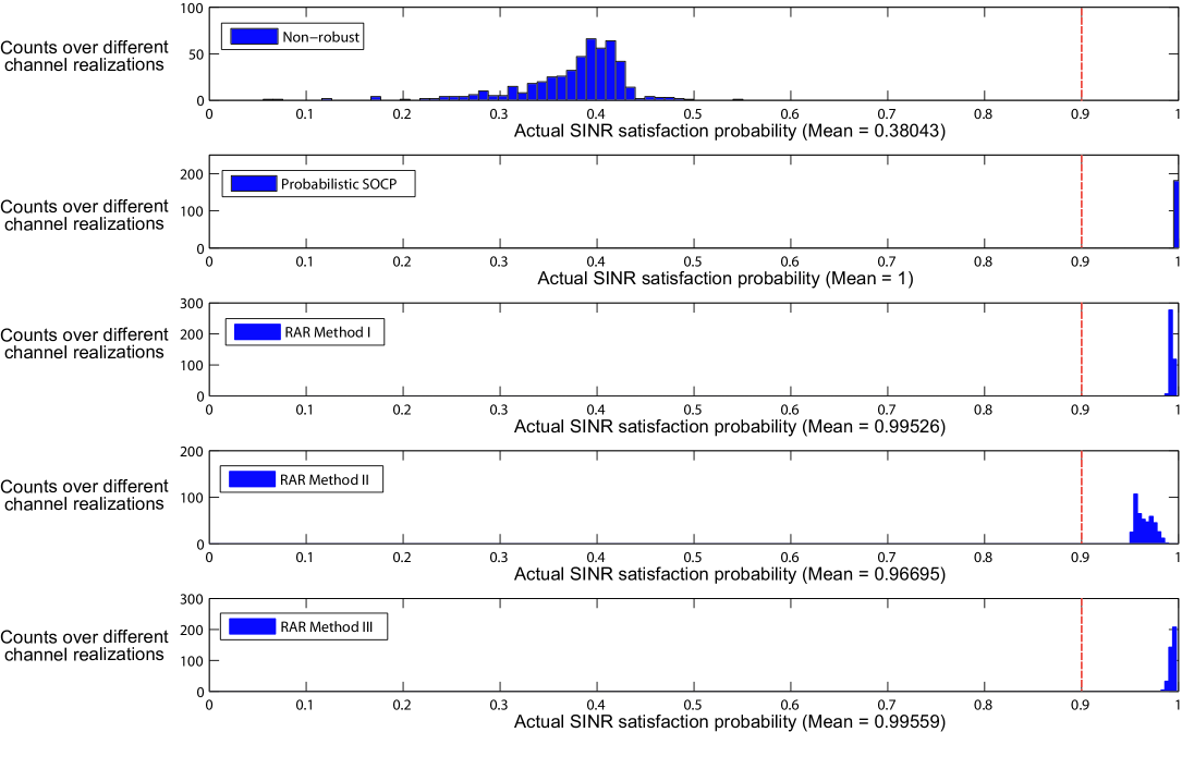
Figure 1: Histograms of the actual SINR satisfaction probabilities of the various methods. $N_{t}=K=3$; ${\bm{C}}_{1}=\cdots={\bm{C}}_{K}=0.002{\bm{I}}_{N_{t}}$; $\gamma=11$ dB; $\rho=0.1$.

First, we are interested in examining the actual SINR satisfaction probability, ${\rm Prob}\{{\sf SINR}_{i}\geq\gamma\}$, of the various methods. Figure 1 shows the histograms of the actual SINR satisfaction probabilities over different channel realizations. To obtain the histograms, we generated $500$ realizations of the presumed channels $\{\bar{}{\bm{h}}_{i}\}_{i=1}^{K}$. Then, for each channel realization, the actual SINR satisfaction probabilities of all methods were numerically evaluated using $10,000$ randomly generated realizations of the CSI errors $\{{\bm{e}}_{i}\}_{i=1}^{K}$, which should be sufficient in terms of the probability evaluation accuracy. Figure 1 validates that our RAR methods (and the existing probabilistic SOCP method) indeed adhere to the $90\%$ SINR satisfaction specification. There are two interesting observations, as can be seen from the figure. The first is with the non-robust method. While the non-robust method is, by nature, expected to violate the SINR outage specification, its actual SINR satisfaction probabilities are below $50\%$ for most of the channel realizations, which is severe. This reveals that the perfect-CSI-based design can be quite sensitive to CSI errors. The second is with the conservatism of the various robust methods. The probabilistic SOCP method has its actual SINR satisfaction probabilities concentrating at $100\%$, which indicates that it may be playing too safe in meeting the outage specification. By contrast, our RAR methods seem to be less conservative. Particularly, among the three methods, RAR Method II (Bernstein-type inequality) appears to be the most relaxed as observed from its histogram.

Next, we investigate the conservatism of the various robust methods by evaluating their feasibility rates; i.e., the chance of getting a feasible beamforming solution under different channel realizations. Similar to the last investigation, $500$ channel realizations were used. The obtained result is shown in Figure 2(a), where the feasibility rates of the various methods are plotted against the SINR requirements $\gamma$. Remarkably, the three RAR methods yield feasibility rates much higher than that of the probabilistic SOCP method. In particular, RAR Method II has the best feasibility rate performance, which is consistent with the SINR satisfaction probability result we noted in Figure 1. The feasibility rates of RAR Methods I and III are a close match: For $\gamma>9$dB, RAR Method I slightly outperforms RAR Method III; for $\gamma\leq 9$dB, we see the converse.

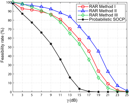
Figure 2: Feasibility and transmit power performance of the various methods. $N_{t}=K=3$; $\rho=0.1$; spatially i.i.d. Gaussian CSI errors with $\sigma_{e}^{2}=0.002$.

In addition to the feasibility rate, it is important to examine the transmit power consumptions of the design solutions offered by the various robust methods. Figure 2(b) shows the result. It was obtained based on channel realizations for which all methods yield feasible solutions at $\gamma=11$dB; $181$ such realizations were found out of $500$ realizations (the same realizations used in the last result in Figure 2(a)). As can be seen from Figure 2(b), RAR Method II yields the best average transmit power performance, followed by RAR Methods I and III (with Method I exhibiting noticeably better performance for $\gamma>15$dB), and then the probabilistic SOCP method in [21]. As a reference, we also plot the transmit powers of the non-robust method in the figure, so as to get an idea of how much additional transmit power would be needed for the robust methods to accommodate the outage specification. We see that for $\gamma\leq 11$dB, the transmit power difference between an RAR method and the non-robust method is about $1.5$dB, which is reasonable especially when compared to the probabilistic SOCP method. The gaps gradually widen, otherwise. This seems to indicate that imperfect CSI effects are more difficult to cope with when we demand higher SINRs.

Now, let us consider the computation times of the various robust methods. The result is illustrated in Figure 3. To obtain this result, we use a desktop PC with $2.13$GHz CPU and $3$GB RAM. Moreover, instead of calling the convenient parser CVX, we use direct SeDuMi implementations of all the methods, done by careful manual problem transformation and programming. The reason of doing so is to bypass parsing overheads, which may result in unfair runtime comparisons. From the figure, we see that the runtime ranking, from the shortest to longest, is: RAR Method III, RAR Method I, RAR Method II, and the probabilistic SOCP method. Interestingly and coincidently, the runtime ranking of the RAR methods is exactly the opposite of their performance ranking we see in the previous simulation result.

\psfrag{Nt=K}[Bc][Bc]{\Large$N_{t}=K$}\includegraphics{Fig3}

Figure 3: Average runtimes of the various methods.

As the last result in this example, we numerically inspect a technical issue that has much implication to the RAR approach— how frequent do the RAR problems yield rank-one solutions. Recall that rank-one RAR solution instances have the benefits that the beamforming solution generation is simple (simple rank-one decomposition, no Gaussian randomization), and that feasibility of the RAR problem directly implies that of beamforming solution generation. Table III shows the result. There is a ratio in each field. The denominator is the realizations count for which the RAR problem is feasible, and the numerator is the realizations count for which the RAR problem yields a rank-one solution. Again, $500$ channel realizations were used. Curiously, almost all the fields in Table III indicate rank-one solution all the time. We encountered only one non-rank-one instance out of $480$ for the setting of $\rho=0.01$, $\gamma=3$dB, RAR Method II. We therefore conclude, on the basis of numerical evidence, that occurrence of high-rank RAR solutions is very rare for the unicast outage-based SINR constrained problem considered here.

TABLE III: Ratios of rank-one RAR solutions.

$\rho$	0.1				0.01
$\gamma$ (dB)	3	7	11	15	3	7	11	15
Method I	464/464	448/448	404/404	292/292	450/450	424/424	343/343	225/225
Method II	489/489	475/475	441/441	363/363	479/480	463/463	428/428	322/322
Method III	488/488	453/453	389/389	267/267	476/476	421/421	306/306	144/144

VI-B Simulation Example 2

This example considers more challenging settings, described as follows: $N_{t}=K=8$; spatially correlated CSI errors where ${\bm{C}}_{1}=\cdots={\bm{C}}_{K}={\bm{C}}_{e}$,

$$[{\bm{C}}_{e}]_{m,n}=\sigma_{e}^{2}\times 0.9^{|m-n|},$$

and $\sigma_{e}^{2}=0.002$; $\rho=0.01$ (or $99\%$ SINR satisfaction probability). We do not run the probabilistic SOCP method in [21], since, as seen in Figure 3, it is computationally very demanding for large problem sizes. The same simulation method in Simulation Example 1 was used to produce the results here. Figure 4 shows the resulting feasible rates and average transmit powers. A minor simulation aspect with the transmit power performance plot in Figure 4(b) is that we choose $\gamma=7$dB as the pick-up point of feasible channel realizations of all the methods. We can see that, once again, RAR Method II offers superior performance over the others. Another observation is that RAR Method III manages to outperform RAR Method I this time.

Figure 5 illustrates another set of results, where we increase the CSI error variance $\sigma_{e}^{2}$ from $0.002$ to $0.01$. The number of users is set to $K=6$. The feasible realizations pick-up point is $\gamma=13$dB. We can see similar performance trends as in the previous result in Figure 4.

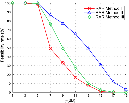
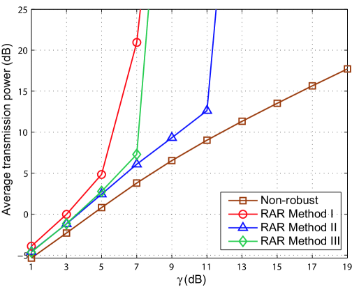
Figure 4: Performance under spatially correlated Gaussian CSI errors. $N_{t}=K=8$; $\rho=0.01$; $\sigma_{e}^{2}=0.002$.

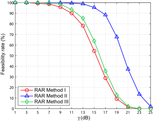
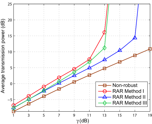
Figure 5: Performance under spatially correlated Gaussian CSI errors. $N_{t}=8$; $K=6$; $\rho=0.01$; $\sigma_{e}^{2}=0.01$.

VI-C Simulation Example 3

One might have noticed from Simulation Example 1, Figure 1, that none of the robust methods yield actual SINR satisfaction probabilities at $1-\rho$. This means that the robust methods are, to certain extent, conservative. If more computations are allowed, this conservatism may be mitigated by running a bisection scheme. Such a scheme was first proposed in [22] in the context of chance constrained optimization, and then was adopted in [21] for the probabilistic SOCP method. The idea is to fine tune some design parameters relevant to the outage requirement. If a design solution is found to satisfy the outage specification well, then we adjust the design parameters to relax the outage requirement (e.g., for RAR Method I, decreasing $d_{1},\ldots,d_{K}$) and rerun the design problem. Otherwise, we do the opposite and rerun the design problem. The above step is done repeatedly following a bisection search, requiring the design problem to be solved multiple times. The bisection search also requires a validation procedure for satisfiability of the outage specification, which can be done using the Monte-Carlo based validation procedure in [22]. It is clear from the above discussion that the bisection scheme can also be applied to all the RAR methods. For more complete descriptions of the bisection scheme in the context of the probabilistic SINR constrained beamforming problem, readers are referred to [21, 1, 2].

Figure 6 shows how bisection may improve the performance. The simulation settings are $N_{t}=K=5$, $\rho=0.1$, ${\bm{C}}_{1}=\cdots={\bm{C}}_{K}=0.002{\bm{I}}_{N_{t}}$, and the feasible realizations pick-up point at $\gamma=9$dB (for the transmit power performance evaluations only). We can see that all the robust methods, after applying the bisection scheme, exhibit improved performance. Notwithstanding, we also see that RAR Method II without bisection already gives performance quite on a par with the bisection-aided methods.

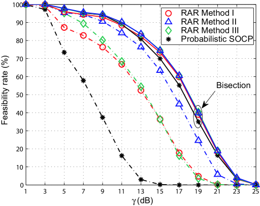
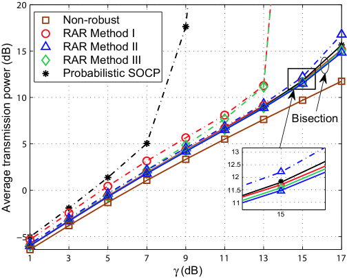
Figure 6: Performance with bisection. $N_{t}=K=5$; $\rho=0.1$; spatially i.i.d. Gaussian CSI errors with $\sigma_{e}^{2}=0.002$.

VI-D Simulation Example 4

This example demonstrates the performance of RAR Method IV, which handles elementwise i.i.d. bounded CSI errors with unknown distribution. We test the method using elementwise i.i.d. uniform CSI errors, where the real and imaginary parts of all ${\bm{e}}_{i}$ are independent and uniformly distributed on $[-\epsilon,\epsilon]$ with $\epsilon>0$. The probabilistic SOCP method in [21] also has a version for i.i.d. uniform CSI errors and is included in our simulation.

The simulation settings are: $N_{t}=K=3$, $\rho=0.1$, $\epsilon=0.02$, and the feasible realizations pick-up point at $\gamma=7$dB. The result, presented in Figure 7, illustrates that RAR Method IV provides much better performance than the probabilistic SOCP method. Table IV shows the ratios of getting a rank-one RAR solution, where we see clearly that encountering high rank RAR solutions is rare.

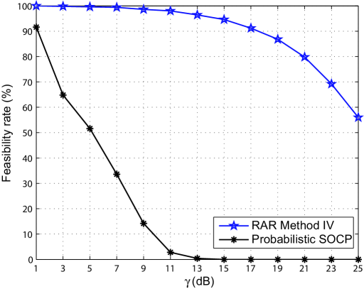
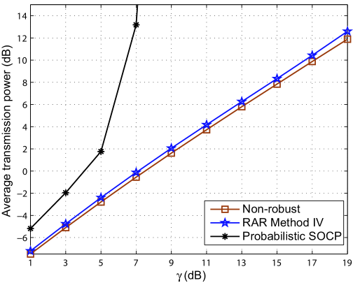
Figure 7: Performance under i.i.d. uniform CSI errors. $N_{t}=K=3$; $\rho=0.1$; $\epsilon=0.02$.

TABLE IV: Ratio of rank-one RAR solutions.

$\gamma$ (dB)	1	3	5	7	9	11	13	15
Method IV	500/500	498/499	498/498	497/497	493/493	490/490	482/482	473/473

VII Conclusions

Motivated by the presence of CSI errors in practical systems and the need to avoid substantial SINR outages among users, we studied a probabilistic SINR constrained formulation of the transmit beamforming design problem. Although such formulation can safeguard each user’s SINR requirement, it is difficult to process computationally due to the SINR outage probability constraints. To circumvent this, we proposed a novel relaxation-restriction (RAR) approach, which features the use of semidefinite relaxation techniques, as well as analytic tools from probability theory, to produce efficiently computable convex approximations of the aforementioned probabilistic formulation. One of our main contributions is the development of three methods— namely, sphere bounding, Bernstein-type inequality, and decomposition— for processing the probabilistic SINR constraints. Our simulation results indicated that the proposed RAR methods provide good approximations to the probabilistic SINR constrained problem, and they significantly improved upon existing methods, both in terms of solution quality and computational complexity.

At the core of our technical development is a set of tools for constructing efficiently computable convex restrictions of chance constraints with quadratic uncertainties. An interesting future direction would be to apply these new tools to other transmit beamforming formulations, such as those arising from the frontier cognitive radio and multicell scenarios, or perhaps even other signal processing applications.

References

- [1] K.-Y. Wang, T.-H. Chang, W.-K. Ma, and C.-Y. Chi, “A semidefinite relaxation based conservative approach to robust transmit beamforming with probabilistic SINR constraints,” in Proc. 18th European Signal Processing Conference (EUSIPCO), Aalborg, Denmark, August 23-27, 2010, pp. 407–411.
- [2] K.-Y. Wang, T.-H. Chang, W.-K. Ma, A. M.-C. So, and C.-Y. Chi, “Probabilistic SINR constrained robust transmit beamforming: A Bernstein-type inequality based conservative approach,” in Proc. IEEE ICASSP 2011, Czech, May 22-27, 2011, pp. 3080–3083.
- [3] A. B. Gershman, N. D. Sidiropoulos, S. Shahbazpanahi, M. Bengtsson, and B. Ottersten, “Convex optimization-based beamforming,” IEEE Signal Process. Mag., vol. 27, no. 3, pp. 62–75, May 2010.
- [4] R. Zhang, Y.-C. Liang, and S. Cui, “Dynamic resource allocation in cognitive radio networks,” IEEE Signal Process. Mag., vol. 27, no. 3, pp. 102–114, May 2010.
- [5] M. Bengtsson and B. Ottersten, “Optimal and suboptimal transmit beamforming,” Chapter 18 in Handbook of Antennas in Wireless Communications, L. C. Godara, Ed., CRC Press, Aug. 2001.
- [6] H. Dahrouj and W. Yu, “Coordinated beamforming for the multicell multi-antenna wireless system,” IEEE Trans. Wireless Commun., vol. 9, no. 5, pp. 1748–1759, May 2010.
- [7] D. Gesbert, S. Hanly, H. Huang, S. S. Shitz, O. Simeone, and W. Yu, “Multi-cell MIMO cooperative networks: A new look at interference,” IEEE J. Sel. Areas Commun., vol. 28, no. 9, pp. 1380–1408, Dec. 2010.
- [8] G. Zheng, K.-K. Wong, and B. Ottersten, “Robust cognitive beamforming with bounded channel uncertainties,” IEEE Trans. Signal Process., vol. 57, pp. 4871–4881, Dec. 2009.
- [9] B. K. Chalise and L. Vandendorpe, “MIMO relay design for multipoint-to-multipoint communications with imperfect channel state information,” IEEE Trans. Signal Process., vol. 57, no. 7, pp. 2785–2796, Jul. 2009.
- [10] F. Rashid-Farrokhi, K. J. R. Liu, and L. Tassiulas, “Transmit beamforming and power control for cellular wireless systems,” IEEE J. Sel. Areas Commun., vol. 16, no. 8, pp. 1437–1450, Oct. 1999.
- [11] M. Schubert and H. Boche, “Solution of the multiuser downlink beamforming problem with individual SINR constraints,” IEEE Trans. Veh. Technol., vol. 53, pp. 18–28, Jan. 2004.
- [12] Y. Huang and D. P. Palomar, “Rank-constrained separable semidefinite programming with applications to optimal beamforming,” IEEE Trans. Signal Process., vol. 58, no. 2, pp. 664–678, Feb. 2010.
- [13] A. Wiesel, Y. C. Eldar, and S. Shamai, “Linear precoding via conic optimization for fixed MIMO receivers,” IEEE Trans. Signal Process., vol. 54, no. 1, pp. 161–176, Jan. 2006.
- [14] D. J. Love, R. W. H. Jr, V. K. N. Lau, D. Gesbert, B. D. Rao, and M. Andrews, “An overview of limited feedback in wireless communication systems,” IEEE J. Sel. Areas Commun., vol. 26, pp. 1341–1365, Oct. 2008.
- [15] M. B. Shenouda and T. N. Davidson, “Convex conic formulations of robust downlink precoder designs with quality of service constraints,” IEEE J. Sel. Topics in Signal Process., vol. 1, pp. 714–724, Dec. 2007.
- [16] N. Vui and H. Boche, “Robust QoS-constrained optimization of downlink multiuser MISO systems,” IEEE Trans. Signal Process., vol. 57, pp. 714–725, Feb. 2009.
- [17] M. B. Shenouda and T. N. Davidson, “Nonlinear and linear broadcasting with QoS requirements: Tractable approaches for bounded channel uncertainties,” IEEE Trans. Signal Process., vol. 57, no. 5, pp. 1936–1947, May 2009.
- [18] G. Zheng, K.-K. Wong, and T.-S. Ng, “Robust linear MIMO in the downlink: A worst-case optimization with ellipsoidal uncertainty regions,” EURASIP J. Adv. Signal Process., vol. 2008, pp. 1–15, Jun. 2008.
- [19] A. Ben-Tal, L. El Ghaoui, and A. Nemirovski, Robust Optimization, ser. Princeton Series in Applied Mathematics. Princeton, NJ: Princeton University Press, 2009.
- [20] N. Vui and H. Boche, “A tractable method for chance-constrained power control in downlink multiuser MISO systems with channel uncertainty,” IEEE Signal Process. Letters, vol. 16, no. 5, pp. 346–349, Apr. 2009.
- [21] M. B. Shenouda and T. N. Davidson, “Probabilistically-constrained approaches to the design of the multiple antenna downlink,” in Proc. 42nd Asilomar Conference 2008, Pacific Grove, October 26-29, 2008, pp. 1120–1124.
- [22] A. Ben-Tal and A. Nemirovski, “On safe tractable approximations of chance-constrained linear matrix inequalities,” Math. Oper. Res., vol. 1, pp. 1–25, Feb. 2009.
- [23] A. M.-C. So, “Moment inequalities for sums of random matrices and their applications in optimization,” 2009, accepted for publication in Math. Prog., available on http://dx.doi.org/10.1007/s10107-009-0330-5.
- [24] M. B. Shenouda and T. N. Davidson, “Outage-based designs for multi-user transceivers,” in Proc. IEEE ICASSP 2009, Taipei, Taiwan, April 19-24, 2009, pp. 2389–2392.
- [25] Z.-Q. Luo, W.-K. Ma, A. M.-C. So, Y. Ye, and S. Zhang, “Semidefinite relaxation of quadratic optimization problems,” IEEE Signal Process. Mag., vol. 27, no. 3, pp. 20–34, May 2010.
- [26] M. Grant and S. Boyd, “CVX: Matlab software for disciplined convex programming,” http://stanford.edu/boyd/cvx, Jun. 2009.
- [27] E. Karipidis, N. D. Sidiropoulos, and Z.-Q. Luo, “Quality of service and max-min fair transmit beamforming to multiple cochannel multicast groups,” IEEE Trans. Signal Process., vol. 53, no. 3, pp. 1268–1279, Mar. 2008.
- [28] A. Ben-Tal and A. Nemirovski, “Robust solutions of linear programming problems contaminated with uncertain data,” Math. Prog., Ser. A, vol. 88, pp. 411–424, 2000.
- [29] D. Bertsimas and M. Sim, “Tractable approximations to robust conic optimization problems,” Math. Prog., Ser. B, vol. 107, pp. 5–36, 2006.
- [30] A. Ben-Tal and A. Nemirovski, Lectures on modern convex optimization: Analysis, algorithms, and engineering applications. Philadelphia: MPS-SIAM Series on Optimization, SIAM, 2001.
- [31] I. Bechar, “A Bernstein-type inequality for stochastic processes of quadratic forms of Gaussian variables,” 2009, preprint, available on http://arxiv.org/abs/0909.3595.
- [32] S.-S. Cheung, A. M.-C. So, and K. Wang, “Chance-constrained linear matrix inequalities with dependent perturbations: A safe tractable approximation approach,” 2011, manuscript, available on http://www.se.cuhk.edu.hk/~manchoso/papers/cclmi_sta.pdf.
- [33] J. F. Sturm, “Using SeDuMi 1.02, a MATLAB toolbox for optimization over symmetric cones,” Optim. Method Softw., vol. 11-12, pp. 625–653, 1999.