Dynamical evolution of a magnetic cloud from the Sun to 5.4 AU

Abstract

Context. Significant quantities of magnetized plasma are transported from the Sun to the interstellar medium via Interplanetary Coronal Mass Ejections (ICMEs). Magnetic Clouds (MCs) are a particular subset of ICMEs, forming large scale magnetic flux ropes. Their evolution in the solar wind is complex and mainly determined by their own magnetic forces and the interaction with the surrounding solar wind.

Aims. In this work we analyze the evolution of a particular MC (observed on March 1998) using in situ observations made by two spacecraft approximately aligned with the Sun, the first one at 1 AU from the Sun and the second one at 5.4 AU. We study the MC expansion, its consequent decrease of magnetic field intensity and mass density, and the possible evolution of the so-called global ideal-MHD invariants.

Methods. We describe the magnetic configuration of the MC at both spacecraft using different models and compute relevant global quantities (magnetic fluxes, helicity and energy) at both helio-distances. We also track back this structure to the Sun, in order to find out its solar source.

Results. We find that the flux rope is significantly distorted at 5.4 AU. However, we are able to analyze the data before the flux rope center is over-passed and compare it with observations at 1 AU. From the observed decay of magnetic field and mass density, we quantify how anisotropic is the expansion, and the consequent deformation of the flux rope in favor of a cross section with an aspect ratio at 5.4 AU of $\approx 1.6$ (larger in the direction perpendicular to the radial direction from the Sun). We quantify the ideal-MHD invariants and magnetic energy at both locations, and find that invariants are almost conserved, while the magnetic energy decays as expected with the expansion rate found.

Conclusions. The use of MHD invariants to link structures at the Sun and the interplanetary medium is supported by the results of this multispacecraft study. We also conclude that the local dimensionless expansion rate, that is computed from the velocity profile observed by a single spacecraft, is very accurate for predicting the evolution of flux ropes in the solar wind.

1 Introduction

Coronal Mass Ejections (CMEs) are explosive events that release energy in the solar atmosphere. The interplanetary counterparts of CMEs are solar wind (SW) structures known as interplanetary coronal mass ejections (ICMEs). Among them there is a subset, called magnetic clouds (MCs), which exhibit a smooth rotation of the magnetic field direction through a large angle, enhanced magnetic field strength, low proton temperature and a low proton plasma beta, $\beta_{p}$. MCs are formed by large scale magnetic flux ropes carrying a large amount of magnetic helicity, magnetic flux and energy away from the Sun. The main characteristics of these structures have been enumerated by Burlaga & Klein (1980).

Several authors have consider MCs as static flux ropes (see, e.g., Goldstein, 1983; Burlaga, 1988; Lepping et al., 1990; Burlaga, 1995; Lynch et al., 2003). Their magnetic fields have been frequently modeled using the Lundquist’s model (Lundquist, 1950), which considers a static and axially-symmetric linear force-free magnetic configuration. Many deviations from this model have been also studied: e.g., non-linear force-free fields (Farrugia et al., 1999), non-force free fields (Mulligan et al., 1999b; Hidalgo et al., 2002; Cid et al., 2002), and several non-cylindrical models (Hu & Sonnerup, 2001; Vandas & Romashets, 2002; Démoulin & Dasso, 2009b), all of them being static. These models are recurrently used to fit in situ magnetic field measurements within MCs to reconstruct the whole flux rope structure. These techniques have also been tested by replacing the observations by the local values found in a numerical simulation, and the output of the models has been compared to the known original full simulation (Riley et al., 2004). The results of these comparisons show that these in situ techniques can reproduce relatively well the magnetic structures when the spacecraft is crossing the MC near its main axis.

In many cases, MCs present clear characteristics of expansion (e.g. Lepping et al., 2003, 2008), so several dynamical models have been developed to describe these clouds during their observation time. Some of these flux rope models suppose a circular cross-section with only a radial expansion (Farrugia et al., 1993; Osherovich et al., 1993b; Farrugia et al., 1997; Shimazu & Marubashi, 2000; Nakwacki et al., 2008b), while other models include expansion in both directions, radial and axial (Shimazu & Vandas, 2002; Berdichevsky et al., 2003; Démoulin & Dasso, 2009a; Nakwacki et al., 2008a). A dynamical model with an elliptical shape was derived by Hidalgo (2003), while a model of the expansion with an anisotropic self-similar expansion in three orthogonal directions was worked out by Démoulin et al. (2008).

From single spacecraft observations we cannot directly infer the global structure of the flux ropes and their evolution through the interplanetary medium because they are one single point local measurements. Several strategies are used to derive more information on MCs with multi-spacecraft data, as follows.

With two spacecraft located at a similar distance from the Sun and separated by a distance of the order of the cross-section of the encountered flux rope, the in situ observations provide data at different parts of the flux rope being negligibly affected by the evolution. This is used to test the technique computing the magnetic field in the cross section from the data of one spacecraft and/or to have a more accurate reconstruction of the magnetic field (Mulligan & Russell, 2001; Liu et al., 2008; Kilpua et al., 2009; Möstl et al., 2009).

When the two spacecraft positions are viewed from the Sun with a significant angle, typically in the interval [10°,80°], one can usually derive an estimation of the extension of the flux rope, or at least an estimation of the extension of the perturbation (e.g. the front shock) induced by the propagation of the flux rope in the interplanetary medium (Cane et al., 1997; Mulligan & Russell, 2001; Reisenfeld et al., 2003). A larger number of spacecraft permits to constrain more the evolving magnetic structure, such as in the case analyzed by Burlaga et al. (1981). Such studies have been extended to cases where the spacecraft are well separated in solar distance with one spacecraft near Earth and the other one at a few AUs (Hammond et al., 1995; Gosling et al., 1995; Liu et al., 2006; Foullon et al., 2007; Rodriguez et al., 2008). They show that large MCs/ICMEs have large scale effects in the heliosphere (e.g. both at low and high latitudes).

When the two spacecraft are separated by spatial scales of the order of one or several AUs, the above analysis should take into account the evolution of the MC with solar distance. This also implies a more difficult association of the in situ observations at both spacecraft. Numerical simulations are then useful tools to check if the events observed at each spacecraft are in fact a unique event (e.g., Riley et al., 2003). Since MCs are moving mostly radially away from the Sun, the radial alignment (line-up) of two spacecraft is a major opportunity to study the radial evolution of a MC, as the MC is crossed at a similar location by the two spacecraft. However, it is not common to find events observed by two nearly radially aligned spacecraft. One case was observed by Helios-1,2 close to 1 AU and later by Voyager-1,2 at 2 AU, with an angular separation from the Sun of about 10° (resp. 23°) between Helios-1 (resp. Helios-2) and both Voyager-1,2 (Burlaga et al., 1981; Osherovich et al., 1993a). A second case was observed by Wind and NEAR spacecraft with an angular separation from the Sun of about 1° and a ratio of solar distances of 1.2 (Mulligan et al., 1999a). A third case was observed by ACE and NEAR spacecraft with an angular separation from the Sun of about 2° and a ratio of solar distances of 1.8 (Mulligan et al., 2001). Finally, a fourth case was observed by ACE and Ulysses spacecraft with an angular separation from the Sun of about 6° and a ratio of solar distances of 5.4 (Skoug et al., 2000; Du et al., 2007). This last case has the advantage of a larger radial separation, so that the evolution has a larger effect. This is the MC selected for a deeper study in this paper.

From the in situ data at different solar distances of the same MC one can infer directly the evolution of the magnetic field and plasma quantities. Such radial evolution is otherwise available only from a statistic analysis of a large number of MCs observed individually at various distances (Liu et al., 2005; Wang et al., 2005a; Leitner et al., 2007; Gulisano et al., 2010), with possible bias coming from the selection of MCs with different properties. Another application of line-up spacecraft is to derive the evolution of global magnetohydrodynamic (MHD) quantities, such as magnetic flux and magnetic helicity (Dasso, 2009). They are main quantities to test if the flux rope simply expands or if a significant part reconnects with the SW field. These global quantities permit also a quantitative link to the related solar event (Mandrini et al., 2005; Luoni et al., 2005; Rodriguez et al., 2008), and set constraints on the physical mechanism of the associated CME launch (Webb et al., 2000; Attrill et al., 2006; Qiu et al., 2007).

In this paper we further analyze the evolution of a MC observed at two different helio-distances, 1 and 5.4 AU (Skoug et al., 2000; Du et al., 2007). This MC has been selected because this is to our knowledge the best line-up observations of a MC between ACE and Ulysses spacecraft. The observations are summarized in Section 2. The velocity and magnetic models used to complement the observations are described in Section 3. This spacecraft line-up is an opportunity to follow the evolution of the flux rope and, in particular, the global MHD quantities such as magnetic helicity and flux (Section 4). We relate this MC to its solar source in Section 5. This complements our understanding of the magnetic field evolution. Finally, we discuss our results and conclude in Section 6.

2 Observations

2.1 Instruments and spacecraft

We analyze data sets for SW plasma and magnetic field from ACE and Ulysses spacecraft. We use the Magnetic Field Experiment (MAG, Smith et al., 1998) with a temporal cadence of 16 seconds and the Solar Wind Electron Proton Alpha Monitor (SWEPAM, McComas et al., 1998) with a temporal cadence of 64 seconds for ACE spacecraft. For Ulysses spacecraft, we use Vector Helium Magnetometer (VHM, Balogh et al., 1992) for magnetic field observations with a temporal cadence of 1 second and Solar Wind Observations Over the Poles of the Sun (SWOOPS, Bame et al., 1992) for plasma observations with a temporal cadence of 4 minutes.

When the MC passed through Earth (March 5, 1998) ACE was located at $\approx 1$ AU in the ecliptic plane, and in a longitude of 164° in the Solar Ecliptic (SE) coordinate system. When the cloud was observed by Ulysses (March 25, 1998), this spacecraft was located at 5.4 AU from the Sun and very near the ecliptic plane, in particular it was at a latitude of 2° and at a longitude of 158°, in the SE system. Thus, the position of both spacecraft differs in 2° for latitude and in 6° for longitude (Skoug et al., 2000; Du et al., 2007). This angular separation corresponds to a separation distance (perpendicular to the radial direction to the Sun) of $\approx 0.6$ AU at the location of Ulysses. This very good alignment between the Sun and both points of observation of the same object, gives us a unique opportunity to observe the same MC at two different evolution stages in the heliosphere.

2.2 Coordinate systems

We analyze ACE data in Geocentric Solar Ecliptic (GSE) system of reference ($\hat{\bf x}_{GSE}$, $\hat{\bf y}_{GSE}$, $\hat{\bf z}_{GSE}$), where $\hat{\bf x}_{GSE}$ points from the Earth toward the Sun, $\hat{\bf y}_{GSE}$ is in the ecliptic plane and in the direction opposite to the planetary motion, and $\hat{\bf z}_{GSE}$ points to the north pole. However, Ulysses data are provided in the heliographic Radial Tangential Normal (RTN) system of reference ($\hat{\bf R}$, $\hat{\bf T}$, $\hat{\bf N}$), in which $\hat{\bf R}$ points from the Sun to the spacecraft, $\hat{\bf T}$ is the cross product of the Sun’s rotation unit vector ($\hat{\bf\Omega}$) with $\hat{\bf R}$, and $\hat{\bf N}$ completes the right-handed system (e.g., Fränz & Harper, 2002).

In order to make an accurate comparison between the observations of vector quantities made from both spacecraft and the orientation of the flux rope at both locations, we rotate all the vectorial data from Ulysses to the local GSE system of ACE (when this spacecraft is at the closest approach distance of the MC axis). We describe this transformation of coordinates in Appendix A. This permits to compare magnetic field components in the same frame (Figs. 1,2), as well as to compare the orientation of the MC at both positions.

We next define a local system of coordinates linked to the cloud (i.e., the cloud frame, Lepping et al., 1990) in order to better understand the cloud properties and to compare the results at both positions (such as the axial/azimuthal magnetic flux). The local axis direction of the MC defines $\hat{\bf z}_{\rm cloud}$ (with $B_{z,\rm cloud}>0$). Since the speed of the cloud is mainly in the Sun-Earth direction and is much larger than the spacecraft speed, which can be supposed to be at rest during the cloud observing time, we assume a rectilinear spacecraft trajectory in the cloud frame. The trajectory defines a direction $\hat{\bf d}$; so, we take $\hat{\bf y}_{\rm cloud}$ in the direction $\hat{\bf z}_{\rm cloud}\times\hat{\bf d}$ and $\hat{\bf x}_{\rm cloud}$ completes the right-handed orthonormal base ($\hat{\bf x}_{\rm cloud},\hat{\bf y}_{\rm cloud},\hat{\bf z}_{\rm cloud}$). Thus, $B_{x,\rm cloud}$, $B_{y,\rm cloud}$, $B_{z,\rm cloud}$ are the components of $\@vec{B}$ in this new base.

The cloud frame is especially useful when the impact parameter, $p$ (the minimum distance from the spacecraft to the cloud axis), is small compared to the MC radius (called $R$ below). In particular, for $p=0$ and a MC described using a cylindrical magnetic configuration, $\@vec{B}(r)=B_{z}(r)\hat{\bf z}+B_{\phi}(r)\hat{\bf\phi}$, we have $\hat{\bf x}_{\rm cloud}=\hat{\bf r}$ and $\hat{\bf y}_{\rm cloud}=\hat{\bf\phi}$ after the spacecraft has crossed the MC axis. In this case, and for a cylindrical flux rope, the magnetic field data obtained by the spacecraft will show: $B_{x,\rm cloud}=0$, a large and coherent variation of $B_{y,\rm cloud}$ (with a change of sign), and an intermediate and coherent variation of $B_{z,\rm cloud}$, from low values at one cloud edge, taking the largest value at its axis and returning to low values at the other edge ($B_{z,\rm cloud}=0$ is typically taken as the MC boundary).

One possible procedure to estimate the flux rope orientation is the classical minimum variance (MV) method applied to the normalized series of magnetic field measurements within the estimated boundaries of the MC (Sonnerup & Cahill, 1967). It was extensively used to estimate the orientation of MCs (see e.g., Lepping et al., 1990; Bothmer & Schwenn, 1998; Farrugia et al., 1999; Dasso et al., 2003; Gulisano et al., 2005) and it provides a good orientation estimation when $p$ is small compared to $R$ and if the in/out bound magnetic fields are not significantly asymmetric. Gulisano et al. (2007) have tested the MV using a static cylindrical Lundquist’s solution. They found a deviation of the axis orientation from the model of typically 3° for $p$ being 30% of $R$. This deviation remains below 20° for $p$ as high as 90% of $R$. Another method to find the MC orientation is called Simultaneous Fitting (SF). It minimizes a residual function, which takes into account the distance between the observed time series of the magnetic field and a theoretical expression containing several free parameters, which include the angles for the flux rope orientation and some physical parameters associated with the physical model assumed for the magnetic configuration in the cloud (e.g. Hidalgo et al., 2002; Dasso et al., 2003).

3 Modeling the magnetic cloud evolution

3.1 Self-similar expansion

The evolution of a MC can be described with the model developed by Démoulin et al. (2008). In this model, based on previous observations and theoretical considerations, a few basic hypothesis are introduced. Firstly, the MC dynamical evolution is split in two different motions: (i) a global one describing the position $\@vec{r}_{CM}(t)=D(t)\hat{\bf v}_{CM}$ of the center of mass (CM) with respect to a fixed heliospheric frame and (ii) an internal expansion where the elements of fluid are described with respect to the CM frame. Secondly, during the spacecraft crossing of the MC, the motion of the MC center is approximately a uniformly accelerated motion and thus

$$D(t)=D_{0}+V_{0}(t-t_{0})+a(t-t_{0})^{2}/2\,.$$ (1)

Thirdly, the cloud coordinate system, ($\hat{\bf x}_{cloud}$, $\hat{\bf y}_{cloud}$, $\hat{\bf z}_{cloud}$) defines the three principal directions of expansion. Fourthly, the expansion of the flux rope is self-similar with different expansion rates in each of the three cloud main axis. In the CM frame, this assumption implies that the position, $\@vec{r}(t)$, of a element of fluid is described by

$$\@vec{r}(t) = x(t)\,\hat{\bf x}_{cloud}+y(t)\,\hat{\bf y}_{cloud}+z(t)\,\hat{\bf z}_{cloud}$$ (2)

$$= x_{0}\,e(t)\,\hat{\bf x}_{cloud}+y_{0}\,f(t)\,\hat{\bf y}_{cloud}+z_{0}\,g(t)\,\hat{\bf z}_{cloud}\,,$$ (3)

where $x(t),y(t),z(t)$ are the fluid coordinates from the CM reference point at time $t$, and where $x_{0},y_{0},z_{0}$ are the position coordinates taken at a reference time $t_{0}$. The time functions $e(t)$, $f(t)$, and $g(t)$, provide the specific time functions for the self-similar evolution. Finally, based on observations of different MCs at different distances from the Sun (e.g., Liu et al., 2005; Wang et al., 2005a; Leitner et al., 2007; Gulisano et al., 2010), we approximate $e(t)$ by the function:

$$e(t)=(D(t)/D_{0})^{l}\,,$$ (4)

and similar expressions for $f(t)$ and $g(t)$, simply replacing the exponent $l$ by $m$ and $n$, respectively, in order to permit an anisotropic expansion. and proton plasma beta ($\beta_{p}$).

From the conservation of mass we model the decay of the proton density as

$$n_{p}=n_{p,0}(D/D_{0})^{-(l+m+n)}\,.$$ (5)

From the kinematic self-similar expansion proposed before, and assuming an ideal evolution (i.e., non-dissipative, so that the magnetic flux across any material surface is conserved), the evolution of the magnetic components advected by the fluid is

$$B_{x,\rm cloud} = B_{x,\rm cloud_{0}}(D/D_{0})^{-(m+n)}\,,$$

$$B_{y,\rm cloud} = B_{y,\rm cloud_{0}}(D/D_{0})^{-(l+n)}\,,$$ (6)

$$B_{z,\rm cloud} = B_{z,\rm cloud_{0}}(D/D_{0})^{-(l+m)}\,.$$

With the above hypothesis and neglecting the evolution of the spacecraft position during the MC observation, the observed velocity profile ($V_{x}$) along the direction $\hat{\bf v}_{CM}$ of the center of mass velocity is expected to be (Démoulin et al., 2008):

$$V_{x} = -V_{0}-a(t-t_{0})+V_{0}\frac{t-t_{0}}{D_{0}/V_{0}+t-t_{0}}\zeta$$ (7)

$$\approx -V_{0}+\frac{V_{0}^{2}}{D_{0}}\zeta(t-t_{0})\,,$$ (8)

where $\gamma$ is the angle between $\hat{\bf z}_{\rm cloud}$ and $\hat{\bf v}_{CM}$ and

$$\zeta=l\sin^{2}\gamma+n\cos^{2}\gamma\,.$$ (9)

For typical values of MCs we can linearize Eq. (7) in $t-t_{0}$ and neglect the acceleration $a$ (Démoulin et al., 2008). This implies that the slope of the observed linear velocity profile provides information on the expansion rate of the flux rope in the two combined directions: $\hat{\bf x}_{cloud}$ and $\hat{\bf z}_{cloud}$ (since $\zeta$ involves both $l$ and $n$).

3.2 Magnetic field

Since MCs have low plasma $\beta$ (a state near to a force free field) and present flux rope signatures, its magnetic configuration is generally modeled using the cylindrical linear force-free field $\@vec{B^{L}}=B_{0}[J_{1}(\alpha_{0}r)\hat{\bf\phi}+J_{0}(\alpha_{0}r)\hat{\bf z}]$ (Lundquist, 1950). If the expansion coefficients in the three main cloud axis ($l,m,n$) would be significantly different, then an initial Lundquist configuration would be strongly deformed. However, observations of the MC field configuration are approximately consistent with this magnetic configuration at different helio-distances, ranging from 0.3 to 5 AU (e.g., Bothmer & Schwenn, 1998; Leitner et al., 2007). So that we expect a small anisotropy on the expansion along different cloud directions (i.e., $l\approx m\approx n$). From observations of different MCs at significantly different helio-distances (Wang et al., 2005b; Leitner et al., 2007) and from observations of the velocity profile slope from single satellite observations (Démoulin et al., 2008; Gulisano et al., 2010), it has been found that $\zeta\approx 0.8$. Since $\zeta$ is a combination of $l$ and $n$, which depends on $\gamma$ for each cloud, a systematic difference on $l$ and $n$ would be detected in a set of MCs with variable $\gamma$ angle. Such systematic variation of $l$ and $n$ with $\gamma$ was not found.

The kinematic self-similar expansion given in the previous section combined with a non-dissipative regime, as expected for space plasmas, provide a prediction for the observed magnetic configuration during the transit of the MC. Then, assuming an initial Lundquist configuration, the observations are modeled as (Démoulin et al., 2008):

$$B_{x,\rm cloud}(t) = -\frac{p}{\rho(t)}\frac{B_{0}}{f(t)g(t)}J_{1}[U(t)]\,,$$ (10)

$$B_{y,\rm cloud}(t) = \frac{V_{\rm c}(t-t_{\rm c})\sin\gamma}{\rho(t)}\frac{B_{0}}{e(t)g(t)}J_{1}[U(t)]\,,$$ (11)

$$B_{z,\rm cloud}(t) = \frac{B_{0}}{e(t)f(t)}J_{0}[U(t)]\,,$$ (12)

and proton plasma beta ($\beta_{p}$). where $U(t)=\frac{\alpha_{0}\rho(t)}{\sqrt{e(t)^{2}+f(t)^{2}}}$, $\rho(t)=\sqrt{(V_{\rm c}(t-t_{\rm c})\sin\gamma)^{2}+p^{2}}$, $B_{0}$ is the strength of the magnetic field and $\alpha_{0}/2$ is the twist of the magnetic field lines near the center, at time $t=t_{\rm c}$. By construction of the self-similar expansion, this magnetic field is divergence free at any time.

Equations (10-12) have free parameters which are computed by fitting these equations to in situ observations, by minimizing a residual function and quantifying the square of the difference between the observed and the predicted value for the magnetic field components (i.e., a least square fit). This provides information on the observed flux rope, such as its orientation, its extension and its magnetic flux. We call this method the Expansion Fitting (EF) method, and EFI method when isotropy ($l=m=n$) is assumed.

3.3 Global magnetic quantities using the Lundquist’s model

Quantification of global magnetic quantities, such as the so-called ideal-MHD invariants, has been very useful to compare and associate MCs and their solar sources (see, e.g., Mandrini et al., 2005; Dasso et al., 2005b; Dasso, 2009). These MHD invariants are computed using a specific model of the MC magnetic configuration (Section 3.2).

For the Lundquist’s solution, the axial flux is

$$F_{z,Lund}=2\pi\int_{0}^{R}B_{z}\,r\,{\mathrm{d}}r=2\pi J_{1}(\alpha_{0}R_{0})\frac{B_{0}R_{0}}{\alpha_{0}}\,,$$ (13)

where $R_{0}$ is the flux rope radius at a reference time $t_{0}$. The azimuthal flux is

$$F_{\varphi,Lund}=L\int_{0}^{R}B_{\varphi}\,{\mathrm{d}}r=(1-J_{0}(\alpha_{0}R_{0}))\frac{B_{0}L_{0}}{\alpha_{0}}\,,$$ (14)

where $L_{0}$ is the axial length of the flux rope at $t_{0}$. For a flux rope staying rooted to the Sun, $L(t)$ is typically of the order of the distance to the Sun $D(t)$.

The relative magnetic helicity is (Dasso et al., 2003; Nakwacki et al., 2008b)

$$H_{Lund} = 4\pi L\int_{0}^{R}A_{\varphi}B_{\varphi}\,r\,{\mathrm{d}}r$$ (15)

$$= 2\pi\left(J_{0}^{2}+J_{1}^{2}-\frac{2J_{0}J_{1}}{\alpha_{0}R_{0}}\right)\frac{L_{0}B_{0}^{2}R_{0}^{2}}{\alpha_{0}}\,.$$ (16)

The magnetic energy content is not an invariant in MCs. In order to compute its decay rate we simplify and assume that the MC expansion is isotropic with $e(t)=f(t)=g(t)$. Then, the magnetic energy ($E_{Lund}$) is computed as (Nakwacki et al., 2008b)

$$E_{Lund}(t) = \frac{2\pi L}{2\mu_{0}}\int_{0}^{R}B^{2}\,r\,{\mathrm{d}}r$$ (17)

$$= \frac{\pi}{e(t)}\left(J_{0}^{2}+J_{1}^{2}-\frac{J_{0}J_{1}}{\alpha_{0}R_{0}}\right)\frac{L_{0}B_{0}^{2}R_{0}^{2}}{\mu_{0}}=\frac{E_{Lund}(t_{0})}{e(t)}\,,$$

where $\mu_{0}$ is the magnetic permeability. Thus, for the isotropic expansion, the magnetic energy decays with time as $e(t)^{-1}$. In the case of a small anisotropic expansion, a similar decay is expected.

3.4 Global magnetic quantities using the direct method

We define below a method to estimate the global magnetic quantities directly from the observations. This method assumes firstly that the cross section is circular, secondly that there is symmetry of translation of $\@vec{B}$ along the main axis of the flux rope, and finally that the impact parameter is low (so that, $B_{y}\approx\pm B_{\phi}$ and $r\approx x$). We also separate the time range covered by the cloud in two branches and proton plasma beta ($\beta_{p}$). (the in-bound/out-bound branches corresponding to the data before/after the closest approach distance to the flux rope axis, see e.g. Dasso et al., 2005a), and we consider each branch in a separate way. We call this method DM-in/DM-out, depending on the branch (in-bound/out-bound) that is used. We define the accumulative magnetic fluxes for the axial and azimuthal field components, in the in-bound branch as

$$F_{z,DM-in}(x) = 2\pi\int_{X_{\rm in}}^{x}B_{z}(x^{\prime})\,x^{\prime}{\mathrm{d}}x^{\prime}$$ (18)

$$F_{y,DM-in}(x) = L\int_{X_{\rm in}}^{x}B_{y}(x^{\prime})\,{\mathrm{d}}x^{\prime}\,,$$ (19)

where $X_{\rm in}$ is the $x$ value at the starting point of the flux rope and ${\mathrm{d}}x=V_{x}\,{\mathrm{d}}t$. Next, from $B_{y}(x)$ and $F_{z,DM-in}(x)$ we obtain an expression for the magnetic helicity (Dasso et al., 2006)

$$H_{DM-in}=2L\int_{X_{\rm in}}^{X_{\rm center}}F_{z,DM-in}(x)\,B_{y}(x)\,x\,{\mathrm{d}}x\,.$$ (20)

Finally, the magnetic energy is computed from the direct observations of $B(t)=|\@vec{B}(t)|$,

$$E_{DM-in}=\frac{\pi L}{\mu_{0}}\int_{X_{\rm in}}^{X_{\rm center}}B^{2}(x)\,x\,{\mathrm{d}}x\,.$$ (21)

In an equivalent way, we define the same quantities for the out-bound branch. These equations are used to estimate these global quantities directly from in situ observations of the magnetic field, using the components of the field and the integration variable ($x$) in the local MC frame.

Table 1: Timings (dd, hh:mm UT) of the interfaces for substructures inside the ICME, identified with numbered ticks in Figures 1-4.

Tick number	Timing-ACE	Timing-Ulysses	Substructure
1	04, 11:00	23, 13:30
			sheath
2	04, 14:30	23, 22:00
			MC in-bound
3	05, 07:45	26, 13:00
			MC out-bound
4	05, 20:30	28, 00:00
			back
5	06, 02:30	28, 09:00

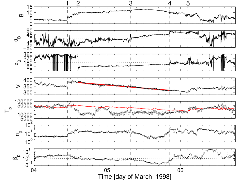
Figure 1: In situ plasma and magnetic field of the ICME observed on March 1998 by ACE located at $\approx 1$ AU from the Sun. From top to bottom: absolute value of the magnetic field ($B=|\@vec{B}|$, in nT), magnetic field vector orientation (GSE): latitude ($\theta_{B}$) and longitude ($\phi_{B}$), bulk velocity ($V$, in km s^-1) including in red the fitted straight line for the MC range (see Section 4.5), the expected (continuous red line) and observed (dots) proton temperature ($T_{p}$, in K), proton density ($n_{p}$, in cm^-3), and proton plasma beta ($\beta_{p}$). Vertical lines mark different interfaces separating different plasma regions (see Section 4.2 for a description and Table 1 for timings). Horizontal dotted lines in $\theta_{B}$, $\phi_{B}$, and $\beta_{p}$ mark values at 0^∘, 180^∘, 1 as a reference, respectively.

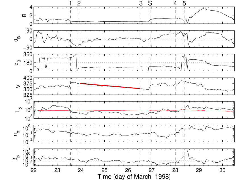
Figure 2: In situ plasma and magnetic field parameters of the ICME observed on March 1998 by Ulysses located at 5.4 AU from the Sun. The format is the same as for Figure 1. The magnetic field components are in the GSE frame defined at ACE (see Section 2.2). Vertical lines with the same reference number correspond to the same interfaces of substructures as at 1 AU.

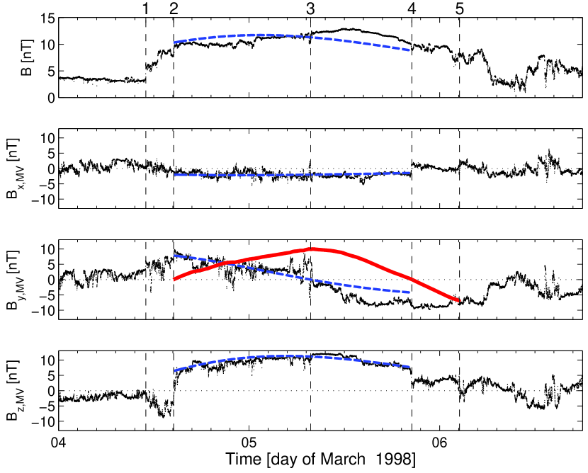
Figure 3: Strength and components of the magnetic field vector at 1 AU in the cloud frame given by the MV method (see Section 4.2). Numbered ticks are the same as in Figure 1. The dashed blue lines are the Lundquist field model fitted with the EFI method (Section 3.2). The red thick line is the accumulative magnetic flux for the azimuthal component (in arbitrary units).

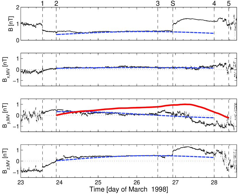
Figure 4: Strength and components of the magnetic field vector at 5.4 AU in the cloud frame given by the MV method applied at 1 AU on ACE data (see Section 4.3). The format is the same as for Figure 3.

4 Results for the studied MC

4.1 Common frame for data at ACE and Ulysses

We first describe the in situ data of both spacecraft in GSE coordinates (defined at the time of ACE observations, see Appendix A). Figure 1 shows the magnetic field and plasma ACE observations. The flux rope extends from ticks ’2’ to ’4’. There, the magnetic field is stronger by a factor $\approx 3$ than in the surrounding SW and it has a coherent rotation. At ACE position the velocity profile is almost linear within the MC (Figure 1). The density is relatively important, up to $\approx 20$ cm^-3, compared to the density present in the SW before the MC sheath, $\approx 5$ cm^-3. In most of the MC the proton temperature is clearly lower than the expected temperature (red line) in a mean SW with the same speed (Lopez & Freeman, 1986; Elliott et al., 2005; Démoulin, 2009); this is a classical property of MCs.

Figure 2 shows Ulysses observations, in the same format as Figure 1. At Ulysses position, the linear velocity profile is still present before a strong shock on March 26, 22:20 UT (tick ’S’ in Figure 2). The proton temperature is, as typically observed in MCs, well below the temperature expected for a typical SW at 5.4 AU from an extrapolation of the empirical law given by Lopez & Freeman (1986). Conversely to ACE, the density is much lower in the MC than in the SW present before the MC sheath ($\approx 0.1-0.2$ cm^-3 in the MC compared to $\approx 0.5-1$ cm^-3 in the SW). With mass conservation, this implies that the volume expansion rate of the MC is much higher than the SW one. The magnetic field observed at Ulysses, has very significantly decreased with respect to the field at ACE (factor $\approx 20$), becoming even weaker than the one present in the surrounding SW (typically by a factor $\approx 2$). This is consistent with the important observed decrease in density.

Table 2: Magnetic cloud orientation according to minimum variance and simultaneous fitting.

Model	Parameter	ACE	Ulysses
Min. Var	$\theta$	12°	-29°
Sim. Fit	$\theta$	-11°	-14°
Min. Var	$\phi$	101°	84°
Sim. Fit	$\phi$	115°	81°

4.2 Magnetic cloud at ACE

The definition of the MC boundaries is an important step in the analysis of a MC since the selected boundaries are affecting all the physical quantities related to the magnetic field. The MC boundaries are associated to discontinuities in the magnetic field because such discontinuities are formed in general at the boundary of two regions having different magnetic connectivities, such as the flux rope and its surrounding medium magnetically linked to the SW.

The front boundary of MCs is typically better defined than the back (or rear) boundary. Such is the case in the analyzed MC at ACE, where there is a fast forward shock at tick ’1’, and a strong discontinuity of $\phi_{B}$ (at tick ’2’ in Figure 1). Moreover, the magnetic field in front has a reverse $\phi_{B}$ and, between ticks ’1’ and ’2’, $\@vec{B}$ is fluctuating, a characteristic of MC sheaths. The density has also a discontinuity and is enhanced just before tick ’2’, another characteristic of MC sheaths. Then, the MC front boundary is set at tick ’2’. It is worth noting that the shock at tick ’1’ was previously identified in Wind spacecraft data at 11:05 UT as an ICME related shock (see http://pwg.gsfc.nasa.gov/wind/current_listIPS.htm). This interplanetary fast forward shock-wave has been recently studied in a multispacecraft analysis by Koval & Szabo (2010). For further details on the characteristics of shocks and their identification in the interplanetary medium see Vinas & Scudder (1986) and Berdichevsky et al. (2000).

The back boundary is also set at a discontinuity of the magnetic field. As typical in MCs, there are several possibilities after 18 UT on March 5 (see Figure 1). However, $\phi_{B}$ and $\theta_{B}$ have clear discontinuities, similar but weaker than the front one, at tick ’4’. This is confirmed by a discontinuity in the density. The above boundaries are used to find the orientation of the flux rope both with the MV and the SF (Section 2.2). Indeed, the MC boundaries are better defined in the MC frame since the axial and azimuthal field components are separated (Figure 3). So we need to determine the MC frame.

We first use the MV method to find the direction of the MC axis. The MV should be applied only to the flux rope, otherwise if part of the back is taken into account the directions given by the MV could be significantly bias (the back region is no longer part of the flux rope at the observation time, Gulisano et al., 2007). Then, an iteration is needed starting with the first estimation of the flux-rope boundaries from the data, performing the MV analysis, then plotting the magnetic field in the cloud coordinates, and finally checking if the selected back boundary is correct with the accumulated azimuthal flux (Eq. (19)). For the studied MC at ACE, the orientation found with the MV provides an almost vanishing accumulated flux at the back boundary selected above (Figure 3). Then, no iteration is needed, and the MV is providing a trustable orientation within the accuracy of the method (Table 2). The small mean value of $B_{x,cloud}$ indicates that the impact parameter is small (Figure 3). This implies that the orientation found by the MV method could differ from the real one by typically $10$°  (Gulisano et al., 2007).

The MC axis direction is also estimated with a standard simultaneous fit (SF) of the Lundquist’s solution to the observations (see end of Section 2.2). The fitting minimizes the distance of the model to the observed magnetic field in a least square manner. As for the MV, it is important to take into account only the data in the range where the flux rope is present. The output of the SF method provides estimations for the MC frame vectors as the MV, and also the impact parameter and the physical parameters (the free parameters of the Lundquist’s solution). There is a significant difference in the MC axis orientations between the MV and the SF methods, larger in latitude (23°) than in longitude (14°). Moreover, with the SF results the accumulated azimuthal flux is significant at the back boundary (so the magnetic flux is not balanced), and there are no nearby significant discontinuities. We conclude that the MV method is providing a better approximation of the MC frame than the SF method in this particular MC. Since $\phi$ is close to 90°, it is a good assumption to consider that ACE crosses the flux rope front (or nose). Moreover since $\theta$ is small, the MC axis lies almost in the ecliptic plane.

In summary, at ACE we select the MC boundaries as March 4, 1998, at 14:30 UT and March 5, 1998, at 20:30. The front boundary differs by up to $\approx 5$h from previous studies. The larger difference is with the back boundary of the MC since it was set on March 06 at 03:15 (Skoug et al., 2000), 2:30 UT (Liu et al., 2005), and 06:30 UT (Du et al., 2007), so significantly later than our boundary set at tick ’4’. Our boundaries take into account the extension of the flux rope when it was crossing ACE. In fact part of the MC characteristics are present after the back boundary ’4’ (e.g. strong and relatively coherent magnetic field, cooler temperature than expected), but some other quantities are closer to typical SW values such as $\beta_{p}$ which is larger than $1$. This was previously found in other MCs (Dasso et al., 2006, 2007), and was called a back region. This type of region was interpreted as formed by a magnetic field and plasma belonging to the flux rope when it was close to the Sun, and later connected to the SW due to magnetic reconnection in the front of the flux rope, which in a low density plasma as the SW could be more efficient due to the Hall effect (e.g., Morales et al., 2005). So a back region has intermediate properties between MC and SW since it is a mixture of the two. Indeed, this is the case at the time of ACE observations since $B_{z,\rm cloud}$ is fluctuating in the back region, while $B_{y,\rm cloud}$ retains more its coherency as in the flux rope (Figure 3).

4.3 Magnetic cloud at Ulysses

At Ulysses the MC has a complex structure in most of the measured parameters. The proton temperature is significantly below the expected temperature in the interval of time between tick ’1’ and about one day after tick ’3’ (Figure 2). At the beginning of this time interval, the magnetic field has a coherent rotation, then later it is nearly constant up to a large discontinuity of the field strength (at tick ’S’, $\approx 0.4$ days after tick ’3’). Later, the magnetic field is stronger with a significant rotation. Then, the observations at Ulysses show a flux rope with characteristics significantly different from a “standard” flux rope such as observed at ACE. A magnetic field strength flatter than at ACE is expected if the flux rope transverse size increases much less rapidly than its length, since it implies that the axial component becomes dominant with increasing distance to the Sun so that the magnetic tension becomes relatively weaker in the force balance (Démoulin & Dasso, 2009a). The strong discontinuity followed by a strong field is more peculiar. Indeed, this MC was strongly overtaken by a faster structure, as shown by the velocity panel of Figure 2, and previously identified by Skoug et al. (2000).

The proton temperature has a similar variation at both spacecraft since it is becoming lower than the expected temperature approximately after the shock defined by the discontinuity of $V$. This discontinuity defines the position of tick ’1’ (Figure 2). The front boundary of the MC is less well defined than at ACE since there is no discontinuity. Still the behavior of the magnetic field is similar at both spacecraft as follows. Before tick ’2’, $\theta_{B}$ is fluctuating while globally decreasing, while after tick ’2’ it is gradually increasing (with fluctuations) at both spacecraft. $\phi_{B}$ has a global behavior similar to a step function at both spacecraft, with nearly constant values both before tick ’1’ and after tick ’2’. The main difference for $\phi_{B}$ is a discontinuity at tick ’2’ at 1 AU, while $\phi_{B}$ has a smooth transition at 5.4 AU. Then, we fix the beginning of the MC, tick ’2’, at the beginning of the period where $\theta_{B}$ starts increasing and $\phi_{B}$ is nearly constant. This is confirmed in the MC frame, as $B_{z,\rm MV}\approx 0$ at tick ’2’ at both 1 and 5.4 AU (Figs. 3,4).

The back boundary is much more difficult to define since there are several possibilities, and the absence of a clear coherence between all the measured parameters. We tried several back boundaries, the MV and the SF methods, and use the iterative method described in Section 4.2 to check the selected boundary in the derived MC cloud frame. We found that the MC axis orientation can change by more than 20° and that the selected boundaries are not confirmed by the cancelation of the accumulated flux.

The difficulties of both the MV and the SF methods are due to the large asymmetry of the MC when observed at Ulysses. Even normalizing the magnetic field strength is not sufficient since the out-bound branch is strongly distorted after the shock (tick ’S’). This is the consequence of the overtaking flow seen after tick ’5’ in Figure 2. The MC observations have characteristics comparable to the MHD simulations of Xiong et al. (2007, 2009) where they modeled the interaction of a flux rope with another faster one. At Ulysses, the internal shock has propagated nearly up to the MC center, so that most of the out bound branch is strongly distorted. This implies that both the MV and the SF methods cannot be used to find the MC orientation at Ulysses.

In the MC frame deduced at ACE, the magnetic field components measured at Ulysses between ticks ’2’ and ’3’ have the expected behavior for a flux rope (Figure 4), as follows. $B_{x,\rm cloud}$ is almost constant and small indicating a low impact parameter. $B_{y,\rm cloud}$ shows a clear rotation and $B_{z,\rm cloud}$ is increasing from tick ’2’ to ’3’. These are indications that the studied MC has not significantly changed its orientation ($\leq$ 10°) between 1 and 5.4 AU, despite the presence of the SW overtaking the rear region of the flux rope. Therefore, for Ulysses we use below the MC frame found at ACE.

The accumulated azimuthal flux is maximum after the internal shock position (Figure 4), an indication that the shock would have overtaken the flux rope center. However, we cannot trust the behavior of the accumulated azimuthal flux behind the shock since the orientation and the strength of the magnetic field are strongly modified. Indeed, all the magnetic field components are perturbed even before the shock, in the interval [’3’,’S’]. Before tick ’3’, $B_{y,\rm cloud}$ is weak and it almost vanishes at tick ’3’, while $B_{z,\rm cloud}$ is nearly maximum there, so we set the flux rope center at tick ’3’.

In summary, at Ulysses we initially select the ICME boundaries, including the sheath, as from March 23 at 13:30 UT (tick ’1’) to March 28 at 09:00 UT (tick ’5’). The boundaries chosen by Skoug et al. (2000) were slightly different since they chose the range from March 24 at 02:00 UT to March 28 at 02:30 UT. The above detailed analysis of the magnetic field behavior indicates that the in-bound branch of the MC is from tick ’2’ to ’3’, with an out-bound branch from ’3’ to ’4’ strongly distorted. The in-bound extension is confirmed by a similar behavior of the velocity and the proton temperature at 1 and 5.4 AU.

4.4 Impact parameter at ACE and Ulysses

The agreement between the characteristics of the MC observed at ACE and Ulysses are clear indications that the same MC was observed. In this section we estimate the impact parameter when the MC is observed at each of the two spacecraft.

Figure 3 shows that $B_{x,cloud}$ is small compared to $B$, as expected when the impact parameter ($p$) is close to zero. From the mean value of $B_{x,cloud}$, we estimate $p/R\approx 0.3$ (see the method in Gulisano et al., 2007). From the in-bound size $S_{ACE,in}$ =0.144 AU and $p/R=0.3$, we estimate that the radius $R_{ACE}\approx 0.15$ AU, with a circular cross-section. Fitting the value of $p/R$, using the SF-EFI method, we also obtain $p/R\approx 0.3$. Another estimation of the impact parameter can be done using the approximation introduced in the simplest form of Eq. (31), $<B_{x,cloud}>/<B>\approx 1.2p/R$ (Démoulin & Dasso, 2009b), assuming a cross section roughly circular. We obtain $p/R\approx 0.27$ from this method. Thus, in conclusion, the impact parameter when ACE observes the cloud is low ($p/R\approx 0.3$) and very similar from its estimation using different proxies.

From the mean value of $B_{x,cloud}$ at Ulysses (see Figure 4), as done for ACE, we estimate $p/R=0.54$. From $S_{Uly,in}$ =0.55 AU and $p/R=0.54$, we estimate that $R_{Uly}\approx 0.65$ AU. The above values of $R$ at both spacecraft are in agreement with the values found from fitting the free parameters of the cylindrical expansion Lundquist model (EFI method, see Section 3.2, Eqs. (10-12)). Again, using also the estimation of the impact parameter from the simplest approximation of Démoulin & Dasso (2009b) ($<B_{x,cloud}>/<B>\approx 1.2p/R$), we obtain from this method that $p/R\approx 0.18$. Thus, in conclusion, the impact parameter when Ulysses observes the cloud is also low, with $p/R$ in the range [0.2-0.5] using different proxies.

Further arguments in favor of the association of the MC observed at ACE and Ulysses are given in the following two sections with the timing and the agreement of the mean velocity, expansion rate, magnetic fluxes and helicity as deduced at the two locations.

4.5 Acceleration and Expansion

The translation velocity of the flux rope at ACE is estimated, as typically done, as the mean value of the observed bulk speed during the observation range [’2’,’4’]. It turns out to be $V_{\rm ACE}=-348$ km/s. However, for Ulysses, because of the perturbation on the out-bound branch, it is not possible to apply this classical procedure. Then, we compute a mean value of the observed speed only in a symmetric range near the center (tick ’3’). We choose a range of 12 hours around ’3’, which gives $V_{\rm Ulysses}=-351$ km/s. So that at Ulysses, the MC travels slightly faster than at ACE, with a mean acceleration of $<\!a\!>=|V_{\rm Ulysses}-V_{\rm ACE}|/\Delta t=0.14\leavevmode\nobreak\$km/s/d, where $\Delta t=21.2$ days is the elapsed time between both centers. However, the small value obtained for the acceleration just indicates that it was almost negligible during the transit from ACE to Ulysses and it implies a negligible contribution to the interpretation of the observed velocity profile as a proxy of the expansion of the flux rope (Eq. (7), see Démoulin et al., 2008, for a justification). Then, we consider below that the MC is traveling from ACE to Ulysses with a constant velocity.

We fit the velocity observations to the velocity model described in Sect. 3.1 (Eq. 8). From the fitted curve (red line, panel 4 Fig. 1 and Fig. 2) we obtain the expansion coefficients $\zeta_{ACE}=0.74$ for ACE and $\zeta_{Uly}=0.67$ for Ulysses. These values are very similar at both helio-distances and they are consistent with previous results found at 1 AU with the same method for a set of 26 MCs (Démoulin et al., 2008), as well as the results obtained from a statistical analysis of MCs or ICMEs observed at various distances of the Sun (Bothmer & Schwenn, 1994; Chen, 1996; Liu et al., 2005; Leitner et al., 2007).

The angle, $\gamma$, between the axis of the MC and the direction of motion defines the contribution of the axial and ortho-radial expansion rate to the observed $v_{x}(t)$, see Eq. (9). From the orientation given by MV at ACE, this angle is $\gamma=101\degr$. This implies that the expansion rate measured from $v_{x}$ is mainly due to the expansion in a direction perpendicular to the cloud axis and, then, for the cloud analyzed here $\zeta\approx l$.

The value of $\zeta$ observed at a given spacecraft, just provides the ’local’ expansion rate, which corresponds to the expansion during the in situ observations. However, since $\zeta_{ACE}\approx\zeta_{Uly}$, we assume that during the full travel between ACE and Ulysses the mean expansion rate occurred at a value between $\zeta=0.67$ and $\zeta=0.74$.

Assuming a self-similar expansion in the Sun-spacecraft direction (as in Eq. (4)), we can link (without any assumptions on the cloud shape and symmetries for the flux rope) the size of the structure along the direction of the MC motion ($\hat{\bf v}_{CM}$), at both helio-distances with the expected size at Ulysses given by $S_{ULY,exp}=S_{ACE,obs}(5.4)^{\zeta}$.

Because the out-bound branch of the MC at Ulysses is strongly distorted, we analyze the in-bound branch. Then, using the mean velocity and the time duration between ticks ’2’ and ’3’, we find that $S_{ACE,in}=$0.144 AU. Then, from the observed value of $\zeta_{ACE}$, we find an expected size at Ulysses of $S_{Uly,exp-in}=$0.498 AU (using the observed $\zeta_{Uly}$, we obtain $S^{\prime}_{Uly,exp-in}=$0.444 AU). This implies an expected center time on March 26, 9:00 UT (and even an earlier time when using $\zeta_{Uly}$). However, the cumulative azimuthal flux ($Fy$, Figure 4 panel 3) is smoothly and monotonically increasing beyond this time, with a strong discontinuity of $By$ a bit later, on March 26, 13:00 UT. At the center of the flux rope we expect a global extreme of $Fy$ (Dasso et al., 2006, 2007; Gulisano et al., 2010), and, in particular, as it was observed when this same cloud was located at 1AU (panel 3 of Figure 3). However, it is not the case in Ulysses at the expected time (9:00 UT), so that we decide to take the center at 13:00 UT, the time when $B_{y}$ started to be disturbed. This lack of exact agreement between the predicted and observed center positions could be associated with the not exact alignment between ACE and Ulysses.

Table 3: Observed (ACE and Ulysses) mean values of proton density ($n_{p}$) and magnetic field ($B$, $B_{y,MV}$, and $B_{z,MV}$) for the in-bound branch of the magnetic cloud, for three different estimations of expansion rates (see Section 4.6). The predicted to observed ratio, at Ulysses, is shown in parenthesis.

Quantity	ACE	Uly	UlyP1	UlyP2	UlyP3
l			0.7	0.7	0.74
m			0.7	1.	1.
$np$ (cm-3)	15.8	0.12	0.27 (2.2)	0.17 (1.4)	0.16 (1.3)
$B$ (nT)	10.3	0.48	0.88 (1.7)	0.56 (1.1)	0.53 (1.0)
$B_{y,MV}$ (nT)	4.1	0.18	0.51 (2.8)	0.24 (1.3)	0.22 (1.2)
$B_{z,MV}$ (nT)	9.0	0.42	0.85 (2.0)	0.51 (1.2)	0.48 (1.2)

4.6 Prediction of the mean plasma density and magnetic field at Ulysses

The expected values of the proton density and magnetic field at Ulysses can be predicted using the observations at ACE and the expansion rates along the three directions ($l$, $m$, and $n$, see Eqs. (5-6)). The mean expansion rate, $\zeta$, along the plasma flow can be estimated with a value between $\zeta_{ACE}$ and $\zeta_{Uly}$, which for the orientation of this cloud results to be $l\approx\zeta$. The presence of bi-directional electrons supports the connectivity of this MC to the Sun (Skoug et al., 2000); then, the axial expansion rate is estimated as $n\approx 1$, because the axial length needs to evolve as $D$ in order to keep the magnetic connectivity of the MC to the Sun (e.g., Démoulin & Dasso, 2009a). For the third expansion rate, $m$, we have no direct observational constraint.

Because after ’S’ at Ulysses (see Figure 2) the cloud is strongly perturbed, we compare ACE and Ulysses in the in-bound branch. Column 2 of Table 3 shows the mean values inside the in-bound branch, for the proton density ($n_{p}$) and the magnetic field observed at ACE. Column 3 shows the same mean values, but now observed at Ulysses. Columns 4-6 show three predictions for these quantities at Ulysses. The field strength, $B$, is computed from $B_{y,MV}$ and $B_{z,MV}$, since $B_{x,MV}$ is dependent on the impact parameter which differs at both spacecraft (anyway $|B_{x,MV}|<<B$ so that including $B_{x,MV}$ does not change significantly the results). All the predictions are made using $n=1$. Column 4 (UlyP1) shows the prediction at Ulysses using $l=(\zeta_{ACE}+\zeta_{Uly})/2=0.7$ and $m=l$ (i.e., an isotropic expansion in the plane perpendicular to the cloud axis). Column 5 (UlyP2) shows the prediction at Ulysses using $l=0.7$ and $m=1$, which corresponds to an expansion such that the cross section of the magnetic cloud is deformed toward an oblate shape in the plane perpendicular to the cloud axis, with the major axis perpendicular to the global flow speed (e.g., Démoulin & Dasso, 2009b). Column 6 (UlyP3) shows the prediction at Ulysses using $l=0.74$ and $m=1$, which corresponds to an expansion in the direction of the plasma main flow as observed at ACE, emulating the case in which the expansion in this direction was similar to that observed at ACE almost all the time.

The assumption $l=0.70$ and $m=l$ (UlyP1) predicts significantly larger values for all the quantities with respect to the observed ones (Table 3). However, the assumption $l=0.70$ and $m=1$ (UlyP2) provides more realistic predictions. Furthermore, the assumption $m=1$, combined with $l=0.74$, gives predictions closer to the observations. Of course due to the lack of a perfect alignment we do not expect an exact matching even when the expansion is well modeled.

Another possible approach is to compute $l,m,n$ from the observed ratio (Ulysses with respect to ACE observations) of the mean values of $n_{p}$, $B_{y,MV}$, and $B_{z,MV}$ in the in-bound. We find $l=0.78$, $m=1.04$, and $n=1.06$. The value of $l$ is close to $\zeta_{ACE}$, measured independently from in situ velocity, and $n$ is close to the expected value obtained with a flux-rope length proportional to the distance to the Sun.

We conclude that the expansion of this cloud between ACE and Ulysses was such that $l\approx\zeta_{ACE}$ and $m\approx n\approx 1$. From this anisotropic expansion, and assuming a circular cross section for the cloud at ACE, we predict an oblate shape at Ulysses with an aspect ratio of the order of $(5.4)^{1-\zeta_{ACE}}\approx 1.55$. If this anisotropic expansion is present also before the cloud reaches 1 AU, this aspect ratio could be even a bit larger.

Table 4: MHD quantities calculated according to each model (see Sect. 3.2). The first column indicates the model, the second shows the name of the global MHD quantities and their units, the next two columns show ACE and Ulysses results, and the last column shows the percentage of decay between ACE and Ulysses results.

Model	Parameter	ACE	Ulysses	% of decay
DM-in	$F_{z}$/Mx $10^{21}$	1.2	0.8	33
EFI	$F_{z}$/Mx $10^{21}$	1.0	0.9	11
DM-in	$F_{y}$/Mx $10^{21}$	2.7	2.5	7
EFI	$F_{y}$/Mx $10^{21}$	2.2	1.9	14
DM-in	$H$/Mx2 $10^{42}$	-6.5	-3.9	40
EFI	$H$/Mx2 $10^{42}$	-2.	-1.8	10
DM-in	$E$/ erg $10^{28}$	18	4.	78
EFI	$E$/ erg $10^{28}$	14.5	3.8	74

4.7 Magnetic fluxes and helicity

From fitting all the free parameters of the expanding model to the observations (method EFI), we compute the global magnetic quantities (Section 3.3, Eqs. (13-17)). We also compute these quantities from the direct observations in the in-bound branch, using the direct method (see Section 3.4, Eqs.  18- 21). We use a length $L=2$ for ACE and $L=10.8$ for Ulysses, because the MC is still connected to the Sun when observed at 1 AU and at 5.4 AU. There is a good agreement between the magnetic fluxes and helicities found at ACE and at Ulysses, with a trend to find slightly lower values at Ulysses, i.e., a small decay of $\approx$ 7-40 $\%$, depending on the method to estimate them (Table 4). We recall that the EFI method uses the full MC observations, so it is less accurate because of the strongly perturbed out-bound branch.

The magnetic energy is not an MHD invariant. In fact, its decay, assuming a self-similar expansion with $l=m=n$, is predicted as $e(t)^{-1}$ (Eq. (17)). For the MC studied here, we expect a decay with a factor $5.4^{-l}$. This factor is in the range $[0.19,0.31]$ for $l$ in the range $[0.7,1.]$. In fact, the results of Section 4.6 indicate that the expansion is anisotropic ($l\approx 0.7$, $m\approx n\approx 1.$). The computation of the energy decay with such anisotropic evolution would require a theoretical development which is outside the scope of this paper. Still, the energy decay is expected to be within the above range. Since the anisotropy in the coefficients $l,m,n$ is relatively small, an approximation of the magnetic energy decay is obtained using a mean expansion of $(l+m+n)/3=0.9$, which implies an energy decay $\approx 0.22$. From the last two rows of Table 4, the observed decay between 1 AU and 5.4 AU is 0.22 and 0.26 for DM and EFI, respectively. There is an excellent agreement with the theoretically expected decay, even when we have simplified the analysis to $l=m=n$ and cylindrical symmetry.

5 Solar source of the MC

5.1 Searching for the solar source

The first step to determine the MC source on the Sun is to delimit the time at which the solar event could have happened. We compute the approximate transit time from Sun to Earth using the MC average velocity at ACE (see Sect. 4.5). Considering that the cloud has travelled $1$ AU at a constant velocity of $V_{\rm c}\approx 350$ km/s (where we neglect the acceleration, which is important only in the first stages of the CME ejection), we find $\tau\approx 1\leavevmode\nobreak\ {\rm AU}/V_{\rm c}\approx 5$ days. As the structure was observed by ACE starting on 4 March, we search for solar ejective events that occurred 5 days before, around 28 February $\pm 1$ day.

From 28 February to 1 March, 1998, 5 numbered active regions (ARs) were present on the solar disk (see top panel of Fig. 5). Only very low X-ray class flares occurred in this period of time, most of them were class B (3 on 27 February, 2 on 28 February, 6 on 1 March) and 3 reached class C on 1 March (see the X-ray light curve from the Geostationary Operational Environmental Satellites in http://www.solarmonitor.org and the corresponding list of events). Two of the latter C-class events occurred in AR 8169 which was located at $\approx$ S21W74 at the time of the flares. We have found no AR associated to the observed B class flares.

We have also looked for the CMEs that occurred from 27 February to 1 March in the catalogue of the Large Angle and Spectroscopic Coronagraph (LASCO, Brueckner et al., 1995) on board the Solar and Heliospheric Observatory (SOHO, see http://cdaw.gsfc.nasa.gov/CME/list). Most CMEs on those days had angular widths not larger than 70° and originated from the eastern solar limb, except for a halo and a partial halo CME.

The halo CME first appeared in LASCO C2 on 27 February at 20:07 UT. This was a poor event inserted in the LASCO catalogue after a revision on January 2006. The CME is clearly visible only in LASCO C2 running difference images (see bottom panel of Fig. 5), in particular after $\approx$ 22:00 UT when its front has already left the C2 field of view (LASCO C2 field of view from 20:07 UT until 22:08 UT is only partial). The speed of the CME leading edge seen in LASCO/C2 and C3 is $\approx 420$ km/s from a linear fit, while a fit with a second order polynomia provides $\approx 340$ km/s at 20 $R_{\sun}$; these values are in agreement with the velocity measured at the front of the MC at ACE ($\approx 385$ km/s), taking into account that the MC velocity is expected to be slightly modified by the interaction with the surrounding wind during its travel to 1 AU. Moreover, a velocity of $\approx 340$ km/s gives a travel time of $\approx 4.5$ days, so as expected.

On the other hand, the partial halo CME first appears in LASCO C2 on 28 February at 12:48 UT. Its central position angle is 236° and its speed from a second order fitting is $\approx 225$ km/s, which is too low considering the MC arrival time at ACE. Furthermore, from an analysis of images of the Extreme Ultraviolet Imaging Telescope (EIT Delaboudiniere et al., 1995) on board SOHO in 195 Å  the CME seems to be a backside event. Therefore, the halo CME is the candidate to be the MC solar counterpart.

To find the source of the halo CME on the Sun, we analyze EIT images obtained on 27 February starting 2 hours before the halo CME appearance in LASCO C2. EIT was working in CME watch mode at that time and, therefore, only images in 195 Å with half spatial resolution and with a temporal cadence of $\approx$ 15 min, or larger, are available. A sequence of 4 images with full spatial resolution in all EIT spectral bands was taken at $\approx$ 07:00 UT, 13:00 UT, 19:00 UT. Furthermore, there is an extended data gap in EIT starting at around 20:00 UT until around 22:00 UT. Considering that all events on 27 February were of very low intensity (a B2.3 flare at $\approx$ 18:20 UT, a B1.5 flare at $\approx$ 19:17 UT, and a B4.3 at $\approx$ 22:55 UT after the halo CME), the low temporal cadence and spatial resolution of EIT images, and the existence of the data gap, we have not been able to unambiguously identify the CME source region. However, from these images and those from the Soft X-ray Telescope (SXT, Tsuneta et al., 1991), it is evident that 2 of the five ARs present on the solar disk displayed signatures of activity (compare, in particular, the image at 20:17 UT with the previous and following one in SXT AlMg movie in http://cdaw.gsfc.nasa.gov/CME_/list/); these are AR 8171 and AR 8164 (see Fig. 5).

From the two ARs that could be the source of the halo CME on 27 February at 20:07 UT, AR 8171 was located at S24E02 which is an appropriate location for a solar region to be the source of a cloud observed at Earth. However, the magnetic flux in this AR is $\approx$ 2.0 $\times$ 10²¹ Mx. This value is small when compared to the range for the axial MC flux measured at ACE (1. - 1.2 $\times$ 10²¹ Mx) since, in general, a MC axial flux is 10% of the AR magnetic flux (Lepping et al., 1997). Furthermore, according to the distribution of the photospheric field of the AR polarities (i.e., the shape of magnetic tongues, see López Fuentes et al., 2000; Luoni et al., 2011, and Fig. 5) the magnetic field helicity in this AR is positive, which is opposite to the MC magnetic helicity sign. Finally, the leading polarity of AR 8171 is negative, and with a positive helicity this implies that the magnetic field component along the polarity inversion line (PIL) points from solar east to west. Since the magnetic field component along the PIL is related to the axial MC field component, this is not compatible with the MC axial field orientation at ACE that points to the solar east (Figure 1). Therefore, we conclude that AR 8171 cannot be the solar source region of the halo CME despite its appropriate location on the disk.

The other possible CME source region is AR 8164, located at N16W32 on 27 February at $\approx$ 20:00 UT. This region is far from the central meridian, considering this location and a radial ejection, one would expect that ACE would have crossed the ejected flux rope eastern leg; however, ACE crossed the MC front (see Section 4.2) which implies that during the ejection the flux rope suffered a deflection towards the east; this probably occurred low in the corona as the CME is a halo. Concerning the AR magnetic flux, its value is $\approx$ 10. $\times$ 10²¹ Mx, which is high enough to explain the MC axial magnetic flux as we discussed previously.

The magnetic helicity sign of AR 8164 is negative, as shown by the shape and evolution of its photospheric polarities in Figure 6 (the spatial organization of the magnetic tongues on 23-25 February). This sign is also confirmed by the coronal field model of the region (see Sect 5.2) and agrees with the MC helicity sign.

Conversely to AR 8171, the leading polarity in AR 8164 is positive, implying a magnetic field component pointing from west to east along the PIL. In this case, this direction is compatible with the orientation of MC axial field. Furthermore, the PIL forms an angle of $\approx 60\degr$ in the clockwise direction with the solar equator, while the MC axis lies almost on the ecliptic (see Sect. 4.2). This difference between the PIL on the Sun and the MC axial direction can be explained by a counter-clockwise rotation of the ejected flux rope, as expected, since its helicity is negative (Török & Kliem, 2005; Green et al., 2007).

From the previous analysis, we conclude that AR 8164 is the most plausible source of the halo CME on 27 February, 1998, which can be the counterpart of the MC observed at ACE on 4-5 March. In the next section we compute the magnetic helicity of the AR before and after the ejection and its variation; this value is used as a proxy of the magnetic helicity carried away from the Sun by the CME.

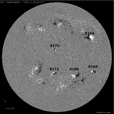
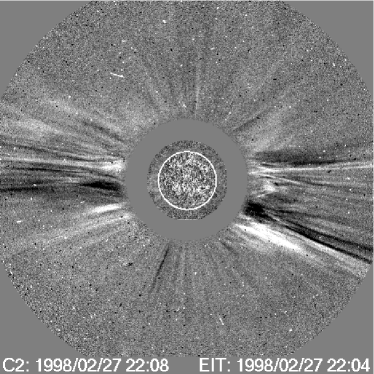
Figure 5: (top) MDI full disk magnetogram on 28 February, 1998, at 00:00 UT (positive/negative magnetic field polarities are indicated in white/black colour). The 5 ARs present on the solar disk are indicated with their NOAA numbers. Notice the location of AR 8171 and AR 8164. The presence of magnetic tongues with a shape compatible with a positive magnetic helicity sign is evident in AR 8171. (bottom) LASCO C2 running difference image showing the halo CME at 22:08 UT together with the closest in time EIT running difference image in 195 Å.

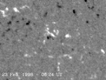
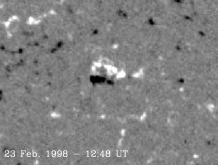
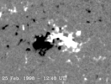
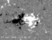
Figure 6: MDI magnetograms of AR 8164 showing the photospheric evolution of its main polarities. The shape and evolution of the magnetic tongues indicates that the magnetic helicity of AR 8164 is negative. The magnetograms have been rotated to the central meridian position of the AR (positive/negative magnetic field polarities are indicated in white/black color). The size of the field of view is the same in all panels.

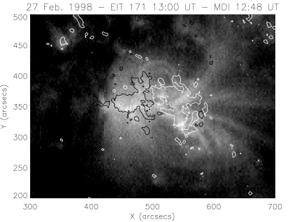
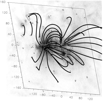
Figure 7: (top) EIT image in 171 Å at 13:00 UT on 27 February, 1998, with two MDI isocontours overlaid ($\pm 100$ G) shown with continuous lines (positive: white line, negative: black line). The MDI magnetogram was taken at 12:48 UT. (bottom) The same EIT image with more isocontours ($\pm$ 100, 500 G) shown with grey lines and computed field lines superimposed (black continuous lines). Both axes are measured in Mm in the local solar frame.

5.2 Physical properties of the solar source

Using AR 8164 MDI magnetograms, we have extrapolated the observed photospheric line of sight component of the field to the corona under the linear (or constant $\alpha$) force-free field assumption: $\@vec{\nabla}\times\@vec{B}=\alpha\@vec{B}$. We have used a fast Fourier transform method as proposed by Alissandrakis (1981) and the transformation of coordinates discussed in Démoulin et al. (1997). The value of $\alpha$ is chosen so as to best fit the observed coronal loops at a given time. We need high spatial resolution images to identify independent loops, which are not available at times close enough before the ejection. Then, we have used the full spatial resolution images obtained by EIT in 171 Å  on 27 February at 13:00 UT; this is the closest time to the event in which coronal loops are visible. The boundary conditions for the model are given by the MDI magnetogram at 12:48 UT on the same day. The value of $\alpha$ is determined through an iterative process that has been explained in Green et al. (2002). The value of $\alpha$ that best fits the observed loops is $\alpha$ = -9.4$\times 10^{-2}$ Mm^-1 (Figure 7).

Once the coronal model is determined, we compute the relative coronal magnetic helicity, $H_{cor}$, following Berger (1985). In particular, we use a linearized version of the expression given by Berger (1985,  see his Eq. A23) as has been done in previous works by Mandrini et al. (2005) and Luoni et al. (2005). Following this approach, the magnetic helicity content in the coronal field before the ejection is $H_{cor}$ = -11.4 $\times$ 10⁴² Mx².

When a flux rope is ejected from the Sun into the IP medium, it carries part of the magnetic helicity contained in the coronal field. Therefore, we have to compute the variation of the coronal magnetic helicity, by subtracting its value before and after an eruptive event, to compare this quantity to the corresponding one in the associated IP event. As done before, we search for an EIT image in 171 Å  with full spatial resolution after the ejection in which loops could be visible. However, in this case, the AR is much closer to the east limb and projection effects, added to the low intensity of the coronal structures, make it even more difficult to distinguish the shape of individual loops; as a result, $\alpha$ cannot be unambiguously determined, i.e. we can adjust the global shape of EIT brightness with more than one $\alpha$ value. We selected the EIT image at 01:20 UT on 28 February and, following a conservative approach, we determine a lower bound for the coronal magnetic helicity variation. We select the closest in time MDI magnetogram (at 01:36 UT on 28 February) and, using the previously determined value for $\alpha$, we compute $H_{cor}$. As the AR magnetic field is decaying, its flux is lower than before the CME ($\approx$ 7.0 $\times$ 10²¹ Mx); therefore, $H_{cor}$ is also lower, $H_{cor}$ = -8.1 $\times$ 10⁴² Mx². The real value of the coronal magnetic helicity after the CME should be even lower than the later one, as we expect that the field relaxes to a closer to potential state. To determine the range of variation for $H_{cor}$, we also compute its value taking the lowest $\alpha$ value ($\alpha$ = -6.3 $\times 10^{-2}$ Mm^-1) that still gives a good fitting to the global shape of EIT brightness after the CME; in this case, $H_{cor}$ = -5.4 $\times$ 10⁴² Mx². Considering the two values determined for $H_{cor}$ after the CME, we estimate that $3.3\times 10^{42}$ Mx² $\leq|\Delta H_{cor}|\leq 6.0\times 10^{42}$ Mx².

5.3 Link with the observed MC

From estimations of the helicity content when the cloud was observed at ACE and Ulysses, using the EFI and DM methods (see Table 4), we found $2\times 10^{42}$ Mx${}^{2}\leq|H_{MC}|\leq 6\times 10^{42}$ Mx², which is fully consistent with the range found for the release of magnetic helicity in the corona during the CME eruption.

A fraction of the total magnetic flux of AR 8164 ($\approx 10\times 10^{21}$ Mx) is enough to account for the magnetic flux in the MC at ACE, $F_{z}$ ($\approx 10^{21}$ Mx) + $F_{y}$ ($\approx 2\times 10^{21}$ Mx) $\approx 3\times 10^{21}$ Mx.

Thus, we have found qualitative and quantitative proofs that let us associate the halo CME observed by LASCO C2 on 27 February, 1998, to its solar source region (AR 8164) and to its interplanetary counterpart, the MC observed at ACE on 4-5 March, 1998, and at Ulysses on 24-28 March, 1998.

6 Summary and Conclusions

We have studied a magnetic cloud which was observed in situ by two spacecraft (ACE and Ulysses) in an almost radial alignment with the Sun ($\approx 2\degr$ for latitude and $\approx 6\degr$ for longitude) and significantly separated in distance (ACE at 1 AU and Ulysses at 5.4 AU). This is an uncommon geometrical scenario and it is very appropriate for multi-spacecraft analysis of MC evolution. In each of the spacecraft locations, we have analyzed the cloud in the local frame (attached to the flux-rope axis) and quantified magnetic fluxes, helicity, and energy, using an expansion model of an initial Lundquist field (EFI) and a direct method (DM), which permits the computation of global magnetic quantities directly from the observed magnetic field (Dasso et al., 2005a). We also computed the local non-dimensional expansion rate ($\zeta$) at ACE and at Ulysses from the observed bulk velocity profiles (as defined in Démoulin et al., 2008).

We found close values of the normalized expansion rate along the solar radial direction, $\zeta_{ACE}=0.74$ and $\zeta_{Uly}=0.67$, as measured from the radial proton velocity at ACE and Ulysses, respectively. From the measured $\zeta_{ACE}$ in the radial direction and assuming a self-similar expansion proportional to the solar distance in the ortho-radial directions, we successfully predicted at Ulysses the values of the MC size, the mean values for density and magnetic field components from the values of these quantities measured at ACE.

Next, comparing observations at Ulysses with different models for anisotropic expansions in the two directions that cannot be directly observed ($m$ and $n$), we found that the expansion on the plane perpendicular to the cloud axis is larger than in the direction perpendicular to the radial direction from the Sun. Based on the quantification of this anisotropic expansion, we conclude that the initial isotropic structure at 1AU will develop an oblate shape such that its aspect ratio would be $\approx 1.6$ at 5.4 AU (i.e., the major axis $\approx 60\%$ larger than the minor one, with the major one perpendicular to the radial direction from the Sun).

From a comparison of the transit time, axis orientation, magnetic fluxes, and magnetic helicity, and considering all the solar sources inside a time window, we have also identified the possible source at the Sun for this event, finding an agreement between the amounts of magnetic fluxes and helicity, in consistence with a rough conservation of these so-called ideal-MHD invariants.

In particular, we found that there is a small decay of the magnetic fluxes and helicity between 1 and 5.4 AU, with a $\approx 10\%$ of decay for $F_{z}$ and $F_{y}$, and a decay of $\approx 10\%$ for the magnetic helicity when the EFI method is used and $\approx 40\%$ when DM is used, respectively. These decays can be due to a possible erosion or pealing of the flux rope during its travel, for instance because of magnetic reconnection with the surrounding SW (e.g., Dasso et al., 2006).

For a self-similar expansion and known expansion rates, it is possible to theoretically derive the decay of the magnetic energy during the travel of the flux rope in the SW. From the observed values of $\zeta$ and modeling the expansion rates in the other two directions ($m$ and $n$), we predict its decay during the travel from 1 AU to 5.4 AU. The measurements confirm this expected magnetic energy decay (from $(15-18)\times 10^{28}$ erg to $4\times 10^{28}$ erg).

Summarizing, in this work we validate for the first time that the local expansion rate ($\zeta$) observed from the velocity profile can be used to make predictions of the decay of mass density and magnetic quantities. From the comparison of detailed predictions and observations of the decays of these quantities, we provide empirical evidence about the quantification of the anisotropic expansion of magnetic clouds beyond Earth, to 5 AUs. Finally, we quantify how much the so-called ideal-MHD invariants are conserved in flux ropes traveling in the solar wind. Then, this kind of combined studies, using multi-spacecraft techniques, is a powerful approach to improve our knowledge of the properties and evolution of magnetized plasma structures ejected from the Sun.

  

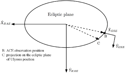
Figure 8: Schema of the positions of each spacecraft at the observed times (left). Schema showing the relationship between the GSE and the HAE system of coordinates (right).

Appendix A Transformation of coordinates between ACE and Ulysses

We describe below the transformation of coordinates between the natural system where the vector data of Ulysses are provided ($\hat{\bf R},\hat{\bf T},\hat{\bf N}$) to the GSE system at the time when the cloud was observed by ACE. Then, we provide a common frame to compare vector observations made at Ulysses and ACE (as shown in Figures 3- 4).

A third coordinate system, the HAE system (Heliocentric Aries Ecliptic, Fränz & Harper (2002)), is used since the location of both spacecraft are known in the HAE system. In this frame, $\hat{\bf Z}_{HAE}$ is normal to the ecliptic plane, and $\hat{\bf X}_{HAE}$ is positive towards the first point of Aries (from Earth to Sun at the vernal equinox, $\approx 21$ March). At the moment in which the cloud was observed by ACE, it was located at a longitude $\epsilon_{A}=163\degr$ and a latitude $\tau_{A}=0\degr$ in the HAE system. When the MC was observed by Ulysses, this spacecraft was located at a longitude of $\epsilon_{U}=157\degr$ and at a latitude of $\tau_{U}=2\degr\$.

The solar equator is defined as the plane normal to the Sun’s rotation vector ($\@vec{\Omega}$) and it is inclined by $\alpha\approx 7.25\degr$ from $\hat{\bf Z}_{HAE}$. In 2000, the solar equator plane intersected the ecliptic plane at a HAE longitude of $\approx 75.6\degr$. Then, the angle between the projection of $\@vec{\Omega}$ on the ecliptic is $\beta\approx 14.4\degr$. When we write $\hat{\bf R}$ and $\@vec{\Omega}$ in the HAE system of coordinates, we obtain:

$$\hat{\bf R} = \cos(\tau_{U})\cos(\epsilon_{U})\leavevmode\nobreak\ \hat{\bf X}_{HAE}+\cos(\tau_{U})\sin(\epsilon_{U})\leavevmode\nobreak\ \hat{\bf Y}_{HAE}$$ (22)

$$+ \sin(\tau_{U})\leavevmode\nobreak\ \hat{\bf Z}_{HAE}\,,$$

$$\@vec{\Omega} = \sin(\alpha)\cos(\beta)\leavevmode\nobreak\ \hat{\bf X}_{HAE}-\sin(\alpha)\sin(\beta)\leavevmode\nobreak\ \hat{\bf Y}_{HAE}$$ (23)

$$+ \cos(\alpha)\leavevmode\nobreak\ \hat{\bf Z}_{HAE}\,.$$

To obtain $\hat{\bf T}$ and $\hat{\bf N}$ at Ulysses in HAE coordinates, we compute:

$$\hat{\bf T} = \frac{\@vec{\Omega}\times\hat{\bf R}}{|\@vec{\Omega}\times\hat{\bf R}|}$$ (24)

$$\hat{\bf N} = \hat{\bf R}\times\hat{\bf T}\,.$$ (25)

To go to the local GSE system of reference we do a last rotation around $\hat{\bf Z}_{HAE}$, which coincides with $\hat{\bf Z}_{GSE}$, in an angle $\delta=180\degr-\epsilon_{A}$ (see Fig. 8).