A passive transmitter for quantum key distribution with coherent light

Abstract

Signal state preparation in quantum key distribution schemes can be realized using either an active or a passive source. Passive sources might be valuable in some scenarios; for instance, in those experimental setups operating at high transmission rates, since no externally driven element is required. Typical passive transmitters involve parametric down-conversion. More recently, it has been shown that phase-randomized coherent pulses also allow passive generation of decoy states and Bennett-Brassard 1984 (BB84) polarization signals, though the combination of both setups in a single passive source is cumbersome. In this paper, we present a complete passive transmitter that prepares decoy-state BB84 signals using coherent light. Our method employs sum-frequency generation together with linear optical components and classical photodetectors. In the asymptotic limit of an infinite long experiment, the resulting secret key rate (per pulse) is comparable to the one delivered by an active decoy-state BB84 setup with an infinite number of decoy settings.

I Introduction

Quantum key distribution (QKD) is already a mature technology that can provide cryptographic systems with an unprecedented level of security qkd . It aims at the distribution of a secret key between two distant parties (typically called Alice and Bob) despite the technological power of an eavesdropper (Eve) who interferes with the signals. This secret key is the essential ingredient of the one-time-pad or Vernam cipher Vernam , the only known encryption method that can offer information-theoretic secure communications.

Most practical long-distance implementations of QKD are based on the so-called BB84 protocol, introduced by Bennett and Brassard in 1984 bb84 , in combination with the decoy-state method decoy ; decoy2 ; decoy2b ; model2 ; decoy_e . In a typical quantum optical implementation of this scheme, Alice sends to Bob phase-randomized weak coherent pulses (WCPs) with different mean photon numbers that are selected, independently and randomly, for each signal. These states can be generated using a standard semiconductor laser together with a variable optical attenuator that is controlled by a random number generator (RNG) random . Each light pulse may be prepared in a different polarization state, which is selected, again independently and randomly for each signal, between two mutually unbiased bases, e.g., either a linear (H [horizontal] or V [vertical]) or a circular (L [left] or R [right]) polarizations basis note . For that, two main experimental configurations are typically used. In the first one, Alice employs four laser diodes, one for each possible BB84 signal 4lasers . These lasers are controlled by a RNG that decides each given time which one of the four diodes is triggered. The second configuration utilizes only one laser diode in combination with a polarization modulator modulator . This modulator rotates the state of polarization of the signals depending on the output of a RNG. On the receiving side, Bob measures each incoming signal by choosing at random between two polarization analyzers, one for each possible basis. Once the quantum communication phase of the protocol is completed, Alice and Bob use an authenticated public channel to process their data and obtain a secure secret key. This last procedure, called key distillation, involves, generally, local randomization, error correction to reconcile Alice’s and Bob’s data, and privacy ampli cation to decouple their data from Eve post . A full proof of the security for the decoy-state BB84 QKD protocol with WCPs has been given in Refs. decoy2 ; decoy2b ; model2 .

Alternatively to the active signal state preparation methods described above, Alice may as well employ a passive transmitter to generate decoy-state BB84 signal states. This last solution might be desirable in some scenarios; for instance, in those experimental setups operating at high transmission rates, since no RNGs are required in a passive device rarity ; passive1 ; passive2 ; passive3 ; passive4 ; passiveEB . Passive schemes could also be more robust against side-channel attacks hidden in the imperfections of the optical components than active sources. The working principle of a passive transmitter is rather simple. For example, Alice can use various light sources to produce different signal states that are sent through an optics network. Depending on the detection pattern observed in some properly located photodetectors, she can infer which signal states are actually generated. Known passive schemes rely typically on the use of a parametric down-conversion (PDC) source, where Alice and Bob passively and randomly choose which bases to measure each incoming pulse by means of a beamsplitter (BS) passiveEB . Also, Alice can exploit the photon number correlations that exist between the two output modes of a PDC source to passively generate decoy states passive1 . More recently, it has been shown that phase-randomized coherent pulses are also suitable for passive preparation of decoy states passive2 ; passive3 and BB84 polarization signals curty , though the combination of both setups in a single passive source is cumbersome. Intuitively speaking, Refs. passive2 ; passive3 ; curty take advantage of the random phase of the different incoming pulses to passively generate states with either distinct photon number statistics but with the same polarization passive2 ; passive3 , or with different polarizations but equal intensities curty .

In this article, we present a complete passive transmitter for QKD that can prepare decoy-state BB84 signal states using coherent light. Our method employs sum-frequency generation (SFG) sfg1 ; kumar together with linear optical components and classical photodetectors. SFG has already exhibited its usefulness in quantum information sfg2 and device-independent QKD sfg3 at the single-photon level. Here we use it in the conventional non-linear optics paradigm with strong coherent light. This fact might render our proposal particularly valuable from an experimental point of view. In the asymptotic limit of an infinite long experiment, it turns out that the secret key rate (per pulse) provided by such passive scheme is similar to the one delivered by an active decoy-state BB84 setup with infinite decoy settings.

The paper is organized as follows. In Sec. II we introduce a passive transmitter that generates decoy-state BB84 polarization signal states using coherent light. Then, in Sec. III we evaluate its performance and we obtain a lower bound on the resulting secret key rate. In Sec. IV we consider the case where Alice and Bob use phase-encoding, which is more suitable to employ in combination with optical fibers than polarization encoding. Finally, Sec. V concludes the article with a summary. The paper includes as well some Appendixes with additional calculations.

II Passive decoy-state BB84 transmitter

The basic setup is illustrated in Fig. 1.

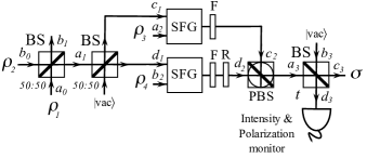
Figure 1: Basic setup of a passive decoy-state BB84 QKD source with polarization encoding using phase-randomized strong coherent pulses. The mean photon number of the signal states $\rho_{i}$, with $i\in\{1,\ldots,4\}$, can be chosen very high; for instance, $\approx{}10^{8}$ photons. BS denotes a beamsplitter, PBS represents a polarizing beamsplitter in the $\pm 45^{\circ}$ linear polarization basis note_last , F is an optical filter, R denotes a polarization rotator changing $+45^{\circ}$ linear polarization to $-45^{\circ}$ linear polarization, $|\rm vac\rangle$ represents the vacuum state, and $t$ denotes the transmittance of a BS; it satisfies $t\ll{}1$.

Let us start considering, for simplicity, the interference of two pure coherent states of frequency $w_{1}$, both prepared in $+45^{\circ}$ linear polarization and with arbitrary phase relationship, $\mbox{$|\sqrt{2\mu}e^{i\theta_{1}}\rangle$}_{a_{0},+45^{\circ}}$ and $\mbox{$|\sqrt{2\mu}e^{i\theta_{2}}\rangle$}_{b_{0},+45^{\circ}}$, at a $50:50$ BS. The output states in modes $a_{1}$ and $b_{1}$ are given by

$$\mbox{$|\sqrt{\mu}(e^{i\theta_{1}}+e^{i\theta_{2}})\rangle$}_{a_{1},+45^{\circ}}\otimes\mbox{$|\sqrt{\mu}(e^{i\theta_{1}}-e^{i\theta_{2}})\rangle$}_{b_{1},+45^{\circ}}.$$ (1)

Then, we have that the output states in modes $c_{1}$ and $d_{1}$ have the form

$$\mbox{$|\sqrt{\frac{\mu}{2}}(e^{i\theta_{1}}+e^{i\theta_{2}})\rangle$}_{c_{1},+45^{\circ}}\otimes\mbox{$|\sqrt{\frac{\mu}{2}}(e^{i\theta_{1}}+e^{i\theta_{2}})\rangle$}_{d_{1},+45^{\circ}}.$$ (2)

If these two states are combined with two coherent states of frequency $w_{2}$, $\mbox{$|\sqrt{\mu}e^{i\theta_{3}}\rangle$}_{a_{2},+45^{\circ}}$ and $\mbox{$|\sqrt{\mu}e^{i\theta_{4}}\rangle$}_{b_{2},+45^{\circ}}$, in a nonlinear medium using the SFG process, the resulting output states at frequency $w_{3}=w_{1}+w_{2}$, after the polarization rotation $R$, can be written as (see Appendix A)

$$\mbox{$|\frac{-\sqrt{\mu}e^{i\theta_{3}}(e^{i\theta_{1}}+e^{i\theta_{2}})}{\sqrt{2}}\rangle$}_{c_{2},+45^{\circ}}\otimes\mbox{$|\frac{-\sqrt{\mu}e^{i\theta_{4}}(e^{i\theta_{1}}+e^{i\theta_{2}})}{\sqrt{2}}\rangle$}_{d_{2},-45^{\circ}}.$$ (3)

These two beams are now re-combined at a PBS in the $\pm 45^{\circ}$ linear polarization basis note_last . We obtain that the output state in mode $a_{3}$ (see Fig. 1) is a coherent state of the form

$$\mbox{$|\sqrt{\zeta(\theta)}e^{i\phi}\rangle$}_{\psi,a_{3}}=e^{-\zeta(\theta)/2}\sum_{n=0}^{\infty}\frac{\big{(}\sqrt{\zeta(\theta)}e^{i\phi}\big{)}^{n}}{\sqrt{n!}}\mbox{$|n_{\psi}\rangle$},$$ (4)

where $\zeta(\theta)=2\mu(1+\cos{\theta})$, $\theta=\theta_{2}-\theta_{1}$, $\phi=\pi+\theta_{1}+\theta_{3}+\arg{(1+e^{i\theta})}$, and the Fock states $|n_{\psi}\rangle$ are given by

$$\mbox{$|n_{\psi}\rangle$}=\frac{[\frac{1}{\sqrt{2}}(a_{+45^{\circ}}^{\dagger}+e^{i\psi}a_{-45^{\circ}}^{\dagger})]^{n}}{\sqrt{n!}}\mbox{$|\rm vac\rangle$},$$ (5)

with $|\rm vac\rangle$ denoting the vacuum state and $\psi=\theta_{4}-\theta_{3}$. Finally, Alice sends the quantum state given by Eq. (4) through a BS of transmittance $t\ll{}1$. Then, the output states in modes $c_{3}$ and $d_{3}$ are given by

$$\mbox{$|\sqrt{t\zeta(\theta)}e^{i\phi}\rangle$}_{\psi,c_{3}}\otimes\mbox{$|\sqrt{(1-t)\zeta(\theta)}e^{i\phi}\rangle$}_{\psi,d_{3}}.$$ (6)

The analysis of the case where the global phase of each input signal $\rho_{i}$, with $i\in\{1,\ldots,4\}$, is randomized and inaccessible to the eavesdropper is now straightforward. It can be solved by just integrating the signals $\mbox{$|\sqrt{t\zeta(\theta)}e^{i\phi}\rangle$}_{\psi,c_{3}}$ and $\mbox{$|\sqrt{(1-t)\zeta(\theta)}e^{i\phi}\rangle$}_{\psi,d_{3}}$ given by Eq. (6) over all angles $\theta,\phi$, and $\psi$. In particular, we have that the output state $\sigma$ in this scenario (see Fig. 1) can be written as

$$\sigma = \frac{1}{(2\pi)^{3}}\iiint_{\phi,\theta,\psi}\mbox{$|\sqrt{t\zeta(\theta)}e^{i\phi}\rangle$}_{\psi,c_{3}}\mbox{$\langle\sqrt{t\zeta(\theta)}e^{i\phi}|$}\ {\rm d}\phi{\rm d}\theta{\rm d}\psi$$ (7)

$$= \frac{1}{(2\pi)^{2}}\int_{\theta}e^{-\gamma(\theta)}\sum_{n=0}^{\infty}\frac{\gamma(\theta)^{n}}{n!}\int_{\psi}\mbox{$|n_{\psi}\rangle$}\mbox{$\langle n_{\psi}|$}\ {\rm d}\theta{\rm d}\psi,$$

where the intensity $\gamma(\theta)$ is given by $\gamma(\theta)=t\zeta(\theta)$.

The weak intensity signal $\sigma$ in mode $c_{3}$ is suitable for QKD and Alice sends it to Bob through the quantum channel. Also, she uses the strong intensity signal available in mode $d_{3}$ to measure both its intensity and polarization. This last measurement can be realized, for example, by means of a passive BB84 detection scheme where the basis choice is performed by a $50:50$ BS, and on each end there is a PBS and two classical photodetectors. From the different intensities observed in each of these four photodetectors, Alice can determine both the value of the angle $\psi$ and the total intensity of the signal. Note that, by assumption, we have that the intensity of the input states $\rho_{i}$ is very high.

For simplicity, let us assume for the moment that the polarization measurement is perfect, i.e., for each incoming signal it provides Alice with a precise value for the measured angle $\psi$, while the intensity measurement only tells her whether the measured intensity is below or above a certain threshold value $\Lambda$ that satisfies $0<\Lambda<4\mu(1-t)$. That is, $\Lambda$ is between the minimal and maximal possible values of the intensity $(1-t)\zeta(\theta)$ of the optical pulses in mode $d_{3}$. The first intensity interval, $\xi_{d}=[0,\Lambda]$, can be associated, for instance, to the generation of a decoy state in output mode $c_{3}$ (that we shall denote as $\sigma_{d}$), while the second intensity interval, $\xi_{s}=[\Lambda,4\mu(1-t)]$, corresponds to the case of preparing a signal state ($\sigma_{s}$). Note, however, that the analysis presented in this section can be straightforwardly adapted to cover as well the case of several intensity intervals $\xi_{i}$ (i.e., the generation of several decoy states). Figure 2 (case A) shows a graphical representation of the intensity $(1-t)\zeta(\theta)$ in mode $d_{3}$ versus the angle $\theta$, together with the threshold value $\Lambda$ and the intensity intervals $\xi_{d}$ and $\xi_{s}$.

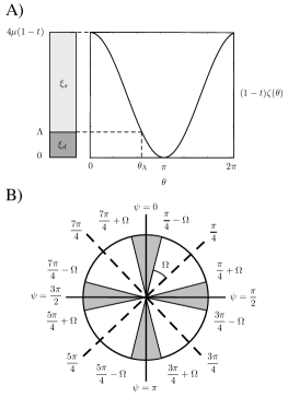
Figure 2: (Case A) Graphical representation of the intensity $(1-t)\zeta(\theta)$ in mode $d_{3}$ (see Fig. 1) versus the angle $\theta$. $\Lambda$ represents the threshold value of the classical intensity measurement, $\theta_{\Lambda}$ is its associated threshold angle, and $\xi_{d}$ and $\xi_{s}$ denote the resulting intensity intervals. (Case B) Graphical representation of the valid regions for the angle $\psi$. These regions are marked in gray. They depend on an acceptance parameter $\Omega\in[0,\pi/4]$.

The threshold angle $\theta_{\Lambda}$ that satisfies $(1-t)\zeta(\theta_{\Lambda})=\Lambda$ is given by

$$\theta_{\Lambda}=\arccos{\Bigg{(}\frac{\Lambda}{2\mu(1-t)}-1\Bigg{)}}.$$ (8)

In this simplified scenario, the conditional quantum states that are sent to Bob can be written as

$$\sigma_{i,\psi}=\sum_{n=0}^{\infty}p_{n}^{i}\mbox{$|n_{\psi}\rangle$}\mbox{$\langle n_{\psi}|$},$$ (9)

where $i=\{s,d\}$, and the probabilities $p_{n}^{i}$ are given by

$$p_{n}^{s} = \frac{1}{\theta_{\Lambda}}\int_{0}^{\theta_{\Lambda}}e^{-\gamma(\theta)}\frac{\gamma(\theta)^{n}}{n!}\ {\rm d}\theta,$$

$$p_{n}^{d} = \frac{1}{\pi-\theta_{\Lambda}}\int_{\theta_{\Lambda}}^{\pi}e^{-\gamma(\theta)}\frac{\gamma(\theta)^{n}}{n!}\ {\rm d}\theta.$$ (10)

In practice, however, it is not necessary that Alice determines the value of $\psi$ accurately and restricts herself to only those events where she actually prepares a perfect BB84 polarization state (i.e., when the angle $\psi$ satisfies $\psi\in\{0,\pi/2,\pi,3\pi/2\}$) curty . Note that the probability associated with these ideal events tends to zero. Instead, it is sufficient if the polarization measurement tells her the value of $\psi$ within a certain interval around the desired ideal values. This situation is illustrated in Fig. 2 (case B), where Alice selects some valid regions (marked with gray color in the figure) for the angle $\psi$ curty . These regions depend on an acceptance parameter $\Omega\in[0,\pi/4]$ that we optimize. In particular, whenever the value of $\psi$ lies within any of the valid regions, Alice considers the pulse emitted by the source as a valid signal. Otherwise, the pulse is discarded afterwards during the post-processing phase of the protocol, and it does not contribute to the key rate. The probability that a pulse is accepted, $p_{\rm acc}$, is given by

$$p_{\rm acc}=1-\frac{4\Omega}{\pi}.$$ (11)

There is a trade-off on the acceptance parameter $\Omega$. A high acceptance probability $p_{\rm acc}$ favors $\Omega\approx{}0$, but this action also results in an increase of the quantum bit error rate (QBER) of the protocol. A low QBER favors $\Omega\approx{}\pi/4$, but then $p_{\rm acc}\approx{}0$. Note that in the limit where $\Omega$ tends to $\pi/4$ we recover the standard decoy-state BB84 protocol.

III Lower bound on the secret key rate

We shall consider that Alice and Bob treat decoy and signal states separately, and they distill secret key from both of them. For that, we use the security analysis presented in Ref. decoy2 , which combines the results provided by Gottesman-Lo-Lütkenhaus-Preskill (GLLP) in Ref. sec_bb84b (see also Ref. hkl ) with the decoy-state method notetor . The secret key rate formula can be written as

$$R\geq{}\sum_{i}p_{i}\ {\rm max}\{R^{i},0\},$$ (12)

with $i=\{s,d\}$. Here $p_{i}$ denotes the probability to generate a state associated to the intensity interval $\xi_{i}$ (i.e., $p_{s}=\theta_{\Lambda}/\pi$ and $p_{d}=1-p_{s}$), and

$$R^{i} \geq {}qp_{\rm acc}\big{\{}-Q^{i}f(E^{i})H(E^{i})+p_{1}^{i}Y_{1}[1-H(e_{1})]$$ (13)

$$+ p_{0}^{i}Y_{0}\big{\}}.$$

The parameter $q$ is the efficiency of the protocol ($q=1/2$ for the standard BB84 scheme, and $q\approx{}1$ for its efficient version eff ); $Q^{i}$ denotes the gain, i.e., the probability that Bob obtains a click in his measurement apparatus when Alice sends him a signal $\sigma_{i}$; $f(E^{i})$ represents the efficiency of the error correction protocol as a function of the error rate $E^{i}$, typically $f(E^{i})\geq{}1$ with Shannon limit $f(E^{i})=1$ gb ; $Y_{n}$ is the yield of an $n$-photon signal, i.e., the conditional probability of a detection event on Bob’s side given that Alice transmits an $n$-photon state; $e_{n}$ denotes the error rate of an $n$-photon signal; and $H(x)=-x\log_{2}{(x)}-(1-x)\log_{2}{(1-x)}$ represents the binary Shannon entropy function.

For simulation purposes, we shall consider a simple channel model in the absence of eavesdropping decoy2 ; model2 ; it just consists of a BS whose transmittance depends on the transmission distance and the loss coefficient of the quantum channel. That is, for simplicity, we neglect any misalignment effect in the channel. Furthermore, we assume that Bob employs an active BB84 detection setup. This model allows us to calculate the observed experimental parameters $Q^{i}$ and $E^{i}$. These quantities are given in Appendix B. Our results, however, can also be straightforwardly applied to any other quantum channel or detection setup, as they depend only on the observed gain and QBER.

To evaluate the secret key rate formula given by Eq. (13) we need to estimate the yields $Y_{0}$ and $Y_{1}$, together with the single-photon error rate $e_{1}$, by solving the following set of linear equations:

$$Q^{i}=\sum_{n=0}^{\infty}p_{n}^{i}Y_{n},\quad{\rm and}\quad Q^{i}E^{i}=\sum_{n=0}^{\infty}p_{n}^{i}Y_{n}e_{n}.$$ (14)

For that, we shall use the procedure proposed in Refs. model2 ; passive3 . Moreover, we will assume a random background (i.e., $e_{0}=1/2$). This method requires that the probabilities $p_{n}^{i}$ given by Eq. (II) satisfy certain conditions that we confirm numerically. The results are included in Appendix C. It is important to emphasize, however, that the estimation technique presented in Refs. model2 ; passive3 only constitutes a possible example of a finite setting estimation procedure. In principle, many other estimation methods are also available for this purpose, such as linear programming tools linear , which might result in sharper, or for the purpose of QKD, better bounds on the considered probabilities.

The resulting lower bound on the secret key rate with two intensity settings is illustrated in Fig. 3 (green line).

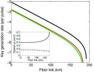
Figure 3: Lower bound on the secret key rate $R$ given by Eq. (12) in logarithmic scale for the passive transmitter with two intensity settings illustrated in Fig. 1 (green line). For simulation purposes, we consider the following experimental parameters: the dark count rate of Bob’s detectors is $\epsilon_{\rm B}=3.2\times 10^{-7}$, the overall transmittance of Bob’s detection apparatus is $\eta_{\rm B}=0.045$, the loss coefficient of the channel is $\alpha=0.2$ dB/km, $q=1/2$, and the efficiency of the error correction protocol is $f(E^{i})=1.22$. We further assume the channel model described in Refs. decoy2 ; model2 , where we neglect any misalignment effect. Otherwise, the actual secure distance will be smaller. The inset figure shows the value for the optimized parameters $\mu{}t$ (dashed line) and $\Omega$ (solid line) in the passive setup. The optimal value for the threshold parameter $\Lambda$ turns out to be constant with the distance and equal to $2\mu(1-t)$, i.e., the threshold angle $\theta_{\Lambda}$ satisfies $\theta_{\Lambda}=\pi/2$. The black line represents a lower bound on $R$ for an active asymptotic decoy-state BB84 system with infinite decoy settings decoy2 , while the red line shows the case of a passive transmitter with infinite intensity intervals $\xi_{i}$ (see Appendix D).

In our simulation we employ the following experimental parameters: the dark count rate of Bob’s detectors is $\epsilon_{\rm B}=3.2\times 10^{-7}$, the overall transmittance of Bob’s detection apparatus is $\eta_{\rm B}=0.045$, and the loss coefficient of the channel is $\alpha=0.2$ dB/km. We further assume that $q=1/2$, and $f(E^{i})=1.22$. With this configuration, it turns out that the optimal value of the parameter $\mu{}t$ decreases with increasing distance, while the optimal value of the parameter $\Omega$ increases with the distance. A similar behavior was also observed in the passive BB84 transmitter (without decoy states) proposed in Ref. curty . In particular, $\mu{}t$ diminishes from $\approx{}0.175$ to $\approx{}0.125$, while $\Omega$ augments from $\approx{}0.393$ to $\approx{}0.7$. At long distances the gain of the protocol is very low and, therefore, it is important to keep both the multi-photon probability of the source (related with the parameter $\mu{}t$) and the intrinsic error rate of the signals sent by Alice (related with the parameter $\Omega$) also low. Figure 3 includes as well an inset plot with the optimized parameters $\mu{}t$ (dashed line) and $\Omega$ (solid line). The optimal value for the parameter $\Lambda$ turns out to be constant with the distance; it is given by $\Lambda=2\mu(1-t)$, i.e., the threshold angle $\theta_{\Lambda}$ is equal to $\pi/2$. This figure also shows a lower bound on the secret key rate for the cases of an active decoy-state BB84 system with infinite decoy settings (black line) decoy2 , and a passive transmitter with infinite intensity intervals $\xi_{i}$ (red line). The cutoff points where the secret key rate drops down to zero are $\approx{}181$ km (passive setup with two intensity settings), $\approx{}183$ km (passive setup with infinite intensity settings), and $\approx{}192$ km (active transmitter with infinite decoy settings). From the results shown in Fig. 3 we see that the performance of the passive transmitter presented in Sec. II, with only two intensity settings, is similar to that of an active asymptotic setup, thus showing the practical interest of the passive scheme. The relatively small difference between the achievable secret key rates in both scenarios is due to two main factors: (a) the intrinsic error rate of the signals accepted by Alice, which is zero only in the case of an active source, and (b) the probability $p_{acc}$ to accept a pulse emitted by the source, which is $p_{acc}<1$ in the passive setup and $p_{acc}=1$ in the active scheme. For instance, we have that for most distances $\Omega\approx{}0.393$, which implies $p_{acc}\approx{}0.5$. This fact reduces the key rate on logarithmic scale of the passive transmitter by a factor of $\log_{10}{p_{acc}}\approx{}0.3$. The additional factor of $\approx{}0.45$ that can be observed in Fig. 3 arises mainly from the intrinsic error rate of the signals.

IV Phase encoding

Similar ideas to the ones presented in Sec. II can also be used in other implementations of the decoy-state BB84 protocol with a different signal encoding. For instance, in those QKD experiments based on phase encoding, which is more suitable to use with optical fibers than polarization encoding, which is particularly relevant in the context of free-space QKD qkd .

The basic setup is illustrated in Fig. 4.

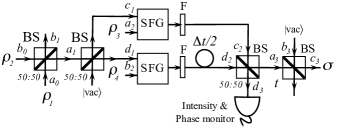
Figure 4: Basic setup of a passive decoy-state BB84 QKD source with phase encoding. The delay introduced by one arm of the interferometer is equal to half the time difference $\Delta{}t$ between two consecutive pulses.

Again, for simplicity, let us consider first the case where the input signals $\rho_{i}$, with $i\in\{1,\ldots,4\}$, are pure coherent states with arbitrary phase relationship: $\mbox{$|\sqrt{2\mu}e^{i\theta_{1}}\rangle$}_{a_{0},+45^{\circ}}$ and $\mbox{$|\sqrt{2\mu}e^{i\theta_{2}}\rangle$}_{b_{0},+45^{\circ}}$ (of frequency $w_{1}$), and $\mbox{$|\sqrt{\mu}e^{i\theta_{3}}\rangle$}_{a_{2},+45^{\circ}}$ and $\mbox{$|\sqrt{\mu}e^{i\theta_{4}}\rangle$}_{b_{2},+45^{\circ}}$ (of frequency $w_{2}$). Let $\Delta{}t$ denote the time difference between two consecutive pulses generated by the sources. Then, from Sec. II we have that the signals in modes $c_{2}$ and $d_{2}$ at time instances $t$ and $t+\Delta{}t/2$ can be written as

$$\mbox{$|\sqrt{\frac{\zeta(\theta)}{2}}e^{i\phi}\rangle$}_{c_{2},+45^{\circ}}^{t}\otimes\mbox{$|\sqrt{\frac{\zeta(\theta)}{2}}e^{i\phi^{\prime}}\rangle$}_{d_{2},+45^{\circ}}^{t+\Delta{}t/2},$$ (15)

where $\phi^{\prime}=\phi+\theta_{4}-\theta_{3}$. Similarly, we find that the quantum states in modes $c_{3}$ and $d_{3}$ are given by, respectively,

$$\mbox{$|\frac{\sqrt{\gamma(\theta)}}{2}e^{i\phi}\rangle$}_{c_{3},+45^{\circ}}^{t} \otimes \mbox{$|\frac{\sqrt{\gamma(\theta)}}{2}e^{i\phi^{\prime}}\rangle$}_{c_{3},+45^{\circ}}^{t+\Delta{}t/2},$$

$$\mbox{$|\frac{\sqrt{\zeta(\theta)}}{2}e^{i\phi}\rangle$}_{d_{3},+45^{\circ}}^{t} \otimes \mbox{$|\frac{\sqrt{\zeta(\theta)}}{2}e^{i\phi^{\prime}}\rangle$}_{d_{3},+45^{\circ}}^{t+\Delta{}t/2}.$$ (16)

The case of phase-randomized strong coherent pulses is completely analogous to that of Sec. II and we omit it here for simplicity; it results in an uniform distribution for the angles $\theta$, $\phi$, and $\phi^{\prime}$ for both pairs of pulses given by Eq. (IV). The strong signals in mode $d_{3}$ are used to measure both their phases, relative to some local reference phase, and their intensities by means of an intensity and phase measurement, while Alice sends the weak signals in mode $c_{3}$ to Bob. Again, just like in the passive source with polarization encoding shown in Fig. 1, Alice can now select some valid regions for the measured phases and also distinguish between different intensity settings. Then, we have that the analysis and results presented in Sec. III also apply straightforwardly to this scenario.

V Conclusion

In this paper, we have introduced a complete passive transmitter for QKD that can prepare decoy-state Bennett-Brassard 1984 signal states using coherent light. Our method employs sum-frequency generation together with linear optical components and classical photodetectors, and constitutes an alternative to those active sources that are typically used in current experimental realizations of QKD. In the asymptotic limit of an infinite long experiment, we have proven that such passive scheme can provide a secret key rate (per pulse) similar to the one delivered by an active decoy-state BB84 setup with infinite decoy settings, thus showing the practical interest of the passive scheme.

The main focus of this paper has been polarization-based realizations of the BB84 protocol, which are particularly relevant for free-space QKD. However, we have also shown that similar ideas can as well be applied to other practical scenarios with different signal encodings, like, for instance, those QKD experiments based on phase encoding, which are more suitable for use in combination with optical fibers.

VI Acknowledgments

We thank F. Steinlechner for helpful discussions. M.C. thanks the University of Toronto for hospitality and support during his stay in this institution. This work was supported by Xunta de Galicia, Spain (grant No. INCITE08PXIB322257PR), by ERDF funds under the project Consolidation of Research Units 2008/075, and by the Ministerio de Educación y Ciencia, Spain (grants TEC2010-14832, FIS2007-60179, FIS2008-01051 and Consolider Ingenio CSD2006-00019).

Appendix A Sum-frequency generation

For completeness, in this Appendix we include the calculations to derive Eq. (3) in Sec. II. Our starting point are the input states to one of the two SFG processes used in the passive transmitter illustrated in Fig. 1: $\mbox{$|\sqrt{\frac{\mu}{2}}(e^{i\theta_{1}}+e^{i\theta_{2}})\rangle$}_{c_{1},+45^{\circ}}$ and $\mbox{$|\sqrt{\mu}e^{i\theta_{3}}\rangle$}_{a_{2},+45^{\circ}}$. Such process is described by the Hamiltonian $H=i\hbar\chi(c_{1}a_{2}c_{2}^{\dagger}-{\rm H.c.})$, where $c_{2}^{\dagger}$ represents the creation operator for the light wave at frequency $w_{3}=w_{1}+w_{2}$ kumar . The parameter $\chi$ is a coupling constant that is proportional to the second-order susceptibility $\chi^{(2)}$ of the nonlinear material, and H.c. denotes a Hermitian conjugate. When the pump mode at frequency $w_{2}$ is kept strong and undepleted, then this mode can be typically treated classically as a complex number. With this assumption, we have that the effective Hamiltonian above can now be written as $H=i\hbar\chi(\sqrt{\mu}e^{i\theta_{3}}c_{1}c_{2}^{\dagger}-{\rm H.c.})$. Using the Heisenberg equation of motion, it is straightforward to obtain the following coupled-mode equations:

$$\frac{{\rm d}c_{1}}{{\rm d}t}=-\chi\sqrt{\mu}e^{-i\theta_{3}}c_{2},\quad\frac{{\rm d}c_{2}}{{\rm d}t}=\chi\sqrt{\mu}e^{i\theta_{3}}c_{1},$$ (17)

which can be solved in terms of initial values at $t=0$ to yield

$$c_{1}(t) = c_{1}(0)\cos{(\sqrt{\mu}\chi{}t)}-e^{-i\theta_{3}}c_{2}(0)\sin{(\sqrt{\mu}\chi{}t)}$$

$$c_{2}(t) = c_{2}(0)\cos{(\sqrt{\mu}\chi{}t)}+e^{i\theta_{3}}c_{1}(0)\sin{(\sqrt{\mu}\chi{}t)}.$$ (18)

At the point of complete conversion, $t_{c}=\pi/(2\sqrt{\mu}\chi)$, we obtain

$$c_{1}^{\dagger}(t_{c})=-e^{i\theta_{3}}c_{2}^{\dagger}(0),\quad c_{2}^{\dagger}(t_{c})=e^{-i\theta_{3}}c_{1}^{\dagger}(0).$$ (19)

That is, at time $t_{c}$ we find that the resulting output state at frequency $w_{3}$ from the SFG process is given by

$$\mbox{$|-\sqrt{\frac{\mu}{2}}e^{i\theta_{3}}(e^{i\theta_{1}}+e^{i\theta_{2}})\rangle$}_{c_{2},+45^{\circ}}.$$ (20)

Appendix B Gain and QBER

In this Appendix, we obtain a mathematical expression for the observed gains $Q^{i}$ and error rates $E^{i}$, with $i\in\{s,d\}$, for the passive QKD transmitter with two intensity settings introduced in Sec. II. For that, we employ the typical channel model in the absence of eavesdropping decoy2 ; model2 ; it just consists of a BS of transmittance $\eta_{\rm channel}=10^{-\frac{\alpha{}d}{10}}$, where $\alpha$ denotes the loss coefficient of the channel measured in dB/km and $d$ is the transmission distance. Moreover, for simplicity, we consider that Bob employs an active BB84 detection setup with two threshold detectors.

The action of Bob’s measurement device can be described by two positive operator value measures (POVMs), one for each of the two BB84 polarization bases $\beta\in\{l,c\}$, with $l$ denoting a linear polarization basis and $c$ a circular polarization basis. Each POVM contains four elements: $G_{\rm vac}^{\beta}$, $G_{\rm 0}^{\beta}$, $G_{\rm 1}^{\beta}$, and $G_{\rm dc}^{\beta}$. The first one corresponds to the case of no click in the detectors, the following two POVM operators give precisely one detection click, and the last one, $G_{\rm dc}^{\beta}$, gives rise to both detectors being triggered. These operators can be written as curty

$$G_{\rm vac}^{\beta} = [1-\epsilon_{\rm B}(2-\epsilon_{\rm B})]F_{\rm vac}^{\beta},$$

$$G_{\rm 0}^{\beta} = (1-\epsilon_{\rm B})\epsilon_{\rm B}F_{\rm vac}^{\beta}+(1-\epsilon_{\rm B})F_{\rm 0}^{\beta},$$

$$G_{\rm 1}^{\beta} = (1-\epsilon_{\rm B})\epsilon_{\rm B}F_{\rm vac}^{\beta}+(1-\epsilon_{\rm B})F_{\rm 1}^{\beta},$$

$$G_{\rm dc}^{\beta} = \openone-G_{\rm vac}^{\beta}-G_{\rm 0}^{\beta}-G_{\rm 1}^{\beta}.$$ (21)

Here we assume that the background rate is, to a good approximation, independent of the signal detection. Moreover, for easiness of notation, we consider only a background contribution coming from the dark count rate $\epsilon_{\rm B}$ of Bob’s detectors and we neglect other background contributions like, for instance, stray light arising from timing pulses which are not completely filtered out in reception. The operators $F_{\rm vac}^{\beta}$, $F_{\rm 0}^{\beta}$, $F_{\rm 1}^{\beta}$, and $F_{\rm dc}^{\beta}$ have the form

$$F_{\rm vac}^{\beta} = \sum_{n,m=0}^{\infty}(1-\eta_{\rm sys})^{n+m}\mbox{$|n,m\rangle$}_{\beta}\mbox{$\langle n,m|$},$$

$$F_{\rm 0}^{\beta} = \sum_{n,m=0}^{\infty}[1-(1-\eta_{\rm sys})^{n}](1-\eta_{\rm sys})^{m}\mbox{$|n,m\rangle$}_{\beta}\mbox{$\langle n,m|$},$$

$$F_{\rm 1}^{\beta} = \sum_{n,m=0}^{\infty}[1-(1-\eta_{\rm sys})^{m}](1-\eta_{\rm sys})^{n}\mbox{$|n,m\rangle$}_{\beta}\mbox{$\langle n,m|$},$$

$$F_{\rm dc}^{\beta} = \sum_{n,m=0}^{\infty}[1-(1-\eta_{\rm sys})^{n}][1-(1-\eta_{\rm sys})^{m}]$$ (22)

$$\times \mbox{$|n,m\rangle$}_{\beta}\mbox{$\langle n,m|$},$$

with $\beta\in\{l,c\}$. The signals $\mbox{$|n,m\rangle$}_{l}$ ($\mbox{$|n,m\rangle$}_{c}$) represent the state which has $n$ photons in the horizontal (circular left) polarization mode and $m$ photons in the vertical (circular right) polarization mode. The parameter $\eta_{\rm sys}$ denotes the overall transmittance of the system. This quantity can be written as $\eta_{\rm sys}=\eta_{\rm B}\eta_{\rm channel}$, where $\eta_{\rm B}$ is the overall transmittance of Bob’s detection apparatus, i.e., it includes the transmittance of any optical component within Bob’s measurement device together with the efficiency of his detectors.

In the scenario considered, it turns out that the gains $Q^{i}$ are independent of the actual polarization of the signals $\sigma_{i,\psi}$ given by Eq. (9) and the basis $\beta$ used to measure them. We obtain

$$Q^{i} = 1-{\rm Tr}\big{(}G_{\rm vac}^{\beta}\sigma_{i,\psi}\big{)}$$ (23)

$$= 1-\frac{(1-\epsilon_{\rm B})^{2}}{p_{i}\pi}\int_{\theta_{\xi_{i}}}e^{-\eta_{\rm sys}\gamma(\theta)}\ {\rm d}\theta,$$

where $p_{s}=\theta_{\Lambda}/\pi$, $p_{d}=1-p_{s}$, $\theta_{\xi_{s}}=[0,\theta_{\Lambda}]$, and $\theta_{\xi_{d}}=[\theta_{\Lambda},\pi]$.

When $\theta_{\Lambda}=\pi/2$, which is the value that maximizes the secret key rate formula given by Eq. (12), we have that the gains $Q^{i}$ can be written as

$$Q^{s} = 1-(1-\epsilon_{\rm B})^{2}A_{-}(\eta_{\rm sys}\zeta),$$

$$Q^{d} = 1-(1-\epsilon_{\rm B})^{2}A_{+}(\eta_{\rm sys}\zeta),$$ (24)

where $\zeta=2\mu{}t$, and

$$A_{\pm}(x)=e^{-x}\big{[}I_{0,x}\pm{}L_{0,x}\big{]}.$$ (25)

Here $I_{q,z}$ represents the modified Bessel function of the first kind, and $L_{q,z}$ denotes the modified Struve function. These functions are defined as Bessel

$$I_{q,z} = \frac{1}{2\pi{}i}\oint e^{(z/2)(t+1/t)}t^{-q-1}dt,$$ (26)

$$L_{q,z} = \frac{z^{q}}{2^{q-1}\sqrt{\pi}\Gamma_{q+1/2}}\int_{0}^{\pi/2}\sinh{(z\cos{\theta})\sin{\theta}^{2q}}d\theta.$$

The error rates $E^{i}$ depend on the value of the angle $\psi$. By symmetry, we can restrict ourselves to evaluate the QBER in only one of the valid regions for $\psi$. Note that is the same in all of them. For instance, let us consider the case where $\psi\in[7\pi/4+\Omega,\pi/4-\Omega]$ (which corresponds to the horizontal polarization interval), and let $E_{\psi}^{i}$ denote the error rate of a signal $\sigma_{i,\psi}$ in that region. This quantity can be written as

$$E_{\psi}^{i}=\frac{1}{Q^{i}}{\rm Tr}\bigg{[}\bigg{(}G_{1}^{l}+\frac{1}{2}G_{\rm dc}^{l}\bigg{)}\sigma_{i,\psi}\bigg{]}.$$ (27)

Here we have considered the typical initial post-processing step in the BB84 protocol, where double-click events are not discarded by Bob, but are randomly assigned to single-click events. Equation (27) can be further simplified as

$$E_{\psi}^{i} = \frac{1}{2Q^{i}}\big{\{}\epsilon_{\rm B}(\epsilon_{\rm B}-1)f_{0,\psi}^{i}+[2+\epsilon_{\rm B}(\epsilon_{\rm B}-3)]f_{1,\psi}^{i}$$ (28)

$$+ (1-\epsilon_{\rm B})^{2}f_{{\rm dc},\psi}^{i}+\epsilon_{\rm B}(2-\epsilon_{\rm B})\big{\}},$$

where $f_{j,\psi}^{i}={\rm Tr}\big{(}F_{j}^{l}\sigma_{i,\psi}^{i}\big{)}$. After a short calculation, we obtain

$$f_{0,\psi}^{i} = \frac{1}{p_{i}\pi}\int_{\theta_{\xi_{i}}}e^{-\eta_{\rm sys}\gamma(\theta)}\Big{[}-1+e^{\frac{1}{2}\eta_{\rm sys}\gamma(\theta)(1+\cos{\psi})}\Big{]}\ {\rm d}\theta,$$

$$f_{1,\psi}^{i} = \frac{1}{p_{i}\pi}\int_{\theta_{\xi_{i}}}e^{-\eta_{\rm sys}\gamma(\theta)}\Big{[}-1+e^{\frac{1}{2}\eta_{\rm sys}\gamma(\theta)(1-\cos{\psi})}\Big{]}\ {\rm d}\theta,$$

$$f_{{\rm dc},\psi}^{i} = 1+\frac{1}{p_{i}\pi}\int_{\theta_{\xi_{i}}}e^{-\eta_{\rm sys}\gamma(\theta)}-e^{-\frac{1}{2}\eta_{\rm sys}\gamma(\theta)(1-\cos{\psi})}$$ (29)

$$- e^{-\frac{1}{2}\eta_{\rm sys}\gamma(\theta)(1+\cos{\psi})}\ {\rm d}\theta.$$

When $\theta_{\Lambda}=\pi/2$, these expressions can be simplified as

$$f_{0,\psi}^{s} = -A_{-}(\eta_{\rm sys}\zeta)+A_{-}[\kappa_{+}(\psi)],$$ (30)

$$f_{0,\psi}^{d} = -A_{+}(\eta_{\rm sys}\zeta)+A_{+}[\kappa_{+}(\psi)],$$

$$f_{1,\psi}^{s} = -A_{-}(\eta_{\rm sys}\zeta)+A_{-}[\kappa_{-}(\psi)],$$

$$f_{1,\psi}^{d} = -A_{+}(\eta_{\rm sys}\zeta)+A_{+}[\kappa_{-}(\psi)],$$

$$f_{{\rm dc},\psi}^{s} = 1+A_{-}(\eta_{\rm sys}\zeta)-A_{-}[\epsilon_{+}(\psi)]-A_{-}[\epsilon_{-}(\psi)],$$

$$f_{{\rm dc},\psi}^{d} = 1+A_{+}(\eta_{\rm sys}\zeta)-A_{+}[\epsilon_{+}(\psi)]-A_{+}[\epsilon_{-}(\psi)],$$

where the parameters $\kappa_{\pm}(\psi)$ and $\epsilon_{\pm}(\psi)$ have the form

$$\kappa_{\pm}(\psi) = \eta_{\rm sys}\zeta[1-(1\pm\cos{\psi})/2],$$

$$\epsilon_{\pm}(\psi) = \eta_{\rm sys}\zeta(1\pm\cos{\psi})/2.$$ (31)

The quantum bit error rates $E^{i}$ are then given by

$$E^{i}=\frac{2}{\pi-4\Omega}\int_{\frac{7\pi}{4}+\Omega}^{\frac{\pi}{4}-\Omega}E_{\psi}^{i}{\rm d}\psi.$$ (32)

Combining Eqs. (28)-(30-32), we find that

$$E^{s} = \frac{1}{2Q^{s}}\Bigg{\{}1-(1-\epsilon_{\rm B})^{2}A_{-}(\eta_{\rm sys}\zeta)+\frac{2}{\pi-4\Omega}\int_{\frac{7\pi}{4}+\Omega}^{\frac{\pi}{4}-\Omega}\epsilon_{\rm B}(\epsilon_{\rm B}-1)A_{-}[\kappa_{+}(\psi)]+[2+\epsilon_{\rm B}(\epsilon_{\rm B}-3)]A_{-}[\kappa_{-}(\psi)]$$

$$- (1-\epsilon_{\rm B})^{2}\big{[}A_{-}[\epsilon_{+}(\psi)]+A_{-}[\epsilon_{-}(\psi)]\big{]}{\rm d}\psi\Bigg{\}},$$

and

$$E^{d} = \frac{1}{2Q^{d}}\Bigg{\{}1-(1-\epsilon_{\rm B})^{2}A_{+}(\eta_{\rm sys}\zeta)+\frac{2}{\pi-4\Omega}\int_{\frac{7\pi}{4}+\Omega}^{\frac{\pi}{4}-\Omega}\epsilon_{\rm B}(\epsilon_{\rm B}-1)A_{+}[\kappa_{+}(\psi)]+[2+\epsilon_{\rm B}(\epsilon_{\rm B}-3)]A_{+}[\kappa_{-}(\psi)]$$ (34)

$$- (1-\epsilon_{\rm B})^{2}\big{[}A_{+}[\epsilon_{+}(\psi)]+A_{+}[\epsilon_{-}(\psi)]\big{]}{\rm d}\psi\Bigg{\}},$$

and we solve these equations numerically.

Appendix C Estimation procedure

The secret key rate formula given by Eq. (13) can be lower bounded by

$$R^{i}\geq{}qp_{\rm acc}\big{\{}-Q^{i}f(E^{i})H(E^{i})+(p_{1}^{i}Y_{1}+p_{0}^{i}Y_{0})[1-H(e_{1}^{U})]\big{\}},$$ (35)

where $e_{1}^{U}$ denotes an upper bound on the single-photon error rate $e_{1}$. Hence, for our purposes, it is enough to obtain a lower bound on the quantities $p^{i}_{1}Y_{1}+p^{i}_{0}Y_{0}$ for all $i\in\{s,d\}$, together with $e_{1}^{U}$. For that, we can directly use the results obtained in Ref. passive3 , which we include in this Appendix for completeness. The probabilities $p_{n}^{i}$ given by Eq. (II) need to satisfy certain conditions that we confirm numerically. In particular, we have that

$$p^{i}_{1}Y_{1}+p^{i}_{0}Y_{0} \geq {}\textrm{max}\Bigg{\{}\frac{p^{i}_{1}(p^{d}_{2}Q^{s}-p^{s}_{2}Q^{d})}{p^{d}_{2}p^{s}_{1}-p^{s}_{2}p^{d}_{1}}$$ (36)

$$+ \Bigg{[}p^{i}_{0}-p^{i}_{1}\frac{p^{d}_{2}p^{s}_{0}-p^{s}_{2}p^{d}_{0}}{p^{d}_{2}p^{s}_{1}-p^{s}_{2}p^{d}_{1}}\Bigg{]}Y_{0}^{U},0\Bigg{\}},$$

where $Y_{0}^{U}$ denotes an upper bound on the background rate $Y_{0}$ given by

$$Y_{0}\leq{}Y_{0}^{U}=\textrm{min}\Bigg{\{}\frac{E^{d}Q^{d}}{p^{d}_{0}e_{0}},\frac{E^{s}Q^{s}}{p^{s}_{0}e_{0}},1\Bigg{\}},$$ (37)

with $e_{0}=1/2$. The single-photon error rate $e_{1}$ can be upper bounded as

$$e_{1}\leq{}e^{U}_{1} = \textrm{min}\Bigg{\{}\frac{E^{d}Q^{d}-p^{d}_{0}Y_{0}^{L}e_{0}}{p^{d}_{1}Y_{1}^{L}},\frac{E^{s}Q^{s}-p^{s}_{0}Y_{0}^{L}e_{0}}{p^{s}_{1}Y_{1}^{L}},$$ (38)

$$\frac{p^{s}_{0}E^{d}Q^{d}-p^{d}_{0}E^{s}Q^{s}}{(p^{d}_{1}p^{s}_{0}-p^{s}_{1}p^{d}_{0})Y_{1}^{L}}\Bigg{\}},$$

where $Y_{1}^{L}$ and $Y_{0}^{L}$ represent, respectively, a lower bound on the yield $Y_{1}$ and the background rate $Y_{0}$. These quantities are given by

$$Y_{1}\geq{}Y^{L}_{1}=\textrm{max}\Bigg{\{}\frac{p^{d}_{2}Q^{s}-p^{s}_{2}Q^{d}-(p^{d}_{2}p^{s}_{0}-p^{s}_{2}p^{d}_{0})Y_{0}^{U}}{p^{d}_{2}p^{s}_{1}-p^{s}_{2}p^{d}_{1}},0\Bigg{\}},$$ (39)

and

$$Y_{0}\geq{}Y^{L}_{0}=\textrm{max}\Bigg{\{}\frac{p^{d}_{1}Q^{s}-p^{s}_{1}Q^{d}}{p^{d}_{1}p^{s}_{0}-p^{s}_{1}p^{d}_{0}},0\Bigg{\}}.$$ (40)

To evaluate these expressions we need the statistics $p_{n}^{i}$ for $n=0,1,2$. Using Eq. (II), and assuming again $\theta_{\Lambda}=\pi/2$, we obtain

$$p^{s}_{0} = A_{-}(\zeta),$$ (41)

$$p^{s}_{1} = \zeta[A_{-}(\zeta)-e^{-\zeta}(I_{1,\zeta}-L_{-1,\zeta})],$$

$$p^{s}_{2} = \frac{\zeta}{2}\Big{\{}\zeta{}A_{-}(\zeta)+e^{-\zeta}\Big{[}\frac{2}{\pi}\Big{(}1-\frac{\zeta^{2}}{3}\Big{)}+(1-2\zeta)(I_{1,\zeta}$$

$$- L_{-1,\zeta})+\zeta(I_{2,\zeta}-L_{2,\zeta})\Big{]}\Big{\}},$$

and

$$p^{d}_{0} = A_{+}(\zeta),$$ (42)

$$p^{d}_{1} = \zeta[A_{+}(\zeta)-e^{-\zeta}(I_{1,\zeta}+L_{-1,\zeta})],$$

$$p^{d}_{2} = \frac{\zeta}{2}\Big{\{}\zeta{}A_{+}(\zeta)+e^{-\zeta}\Big{[}-\frac{2}{\pi}\Big{(}1-\frac{\zeta^{2}}{3}\Big{)}+(1-2\zeta)(I_{1,\zeta}$$

$$+ L_{-1,\zeta})+\zeta(I_{2,\zeta}+L_{2,\zeta})\Big{]}\Big{\}}.$$

Appendix D Asymptotic passive decoy-state BB84 transmitter

To evaluate the secret key rate formula given by Eq. (12) in this scenario, we consider that $p_{s}\approx{}1$, and we assume that Alice and Bob can estimate the relevant parameters $Y_{0}$, $Y_{1}$, and $e_{1}$ perfectly. Moreover, we use the channel and detection models introduced in Appendix B. In this situation, it turns out that the yields $Y_{0}$ and $Y_{1}$ are given by $Y_{0}=\epsilon_{\rm B}(2-\epsilon_{\rm B})$ and $Y_{1}=1-(1-Y_{0})(1-\eta_{\rm sys})$.

The single-photon error rate $e_{1}$ can be calculated using Eqs. (28)-(32) with $\sigma_{i,\psi}=\mbox{$|1_{\psi}\rangle$}\mbox{$\langle 1_{\psi}|$}$. After a short calculation, we obtain

$$e_{1} = \frac{1}{2Y_{1}}\Bigg{\{}Y_{0}+(1-\epsilon_{\rm B})^{2}\eta_{\rm sys}-\frac{4(1-\epsilon_{\rm B})\eta_{\rm sys}}{\pi-4\Omega}$$ (43)

$$\times \sin{\bigg{(}\frac{\pi}{4}-\Omega\bigg{)}}\Bigg{\}}.$$

The resulting lower bound on the secret key rate is illustrated in Fig. 3 (red line) for the optimized parameters $\zeta$ and $\Omega$.

References

• (1) N. Gisin, G. Ribordy, W. Tittel and H. Zbinden, Rev. Mod. Phys. 74, 145 (2002); M. Dušek, N. Lütkenhaus and M. Hendrych, Progress in Optics 49, Edt. E. Wolf (Elsevier), 381 (2006); V. Scarani, H. Bechmann-Pasquinucci, N. J. Cerf, M. Dušek, N. Lütkenhaus and M. Peev, Rev. Mod. Phys. 81, 1301 (2009).
• (2) G. S. Vernam, J. Am. Inst. Electr. Eng. XLV, 109 (1926).
• (3) C. H. Bennett and G. Brassard, Proc. IEEE Int. Conference on Computers, Systems and Signal Processing, Bangalore, India, IEEE Press, New York, 175 (1984).
• (4) W.-Y. Hwang, Phys. Rev. Lett. 91, 057901 (2003).
• (5) H.-K. Lo, X. Ma and K. Chen, Phys. Rev. Lett. 94, 230504 (2005).
• (6) X.-B. Wang, Phys. Rev. Lett. 94, 230503 (2005); X.-B. Wang, Phys. Rev. A 72, 012322 (2005); X.-B. Wang, Phys. Rev. A 72, 049908(E) (2005).
• (7) X. Ma, B. Qi, Y. Zhao and H.-K- Lo, Phys. Rev. A 72, 012326 (2005).
• (8) Y. Zhao, B. Qi, X. Ma, H.-K. Lo and L. Qian, Phys. Rev. Lett. 96, 070502 (2006); Y. Zhao, B. Qi, X. Ma, H.-K. Lo and L. Qian, Proc. of IEEE International Symposium on Information Theory (ISIT’06), 2094 (2006); C.-Z. Peng, J. Zhang, D. Yang, W.-B. Gao, H.-X. Ma, H. Yin, H.-P. Zeng, T. Yang, X.-B. Wang and J.-W. Pan, Phys. Rev. Lett. 98, 010505 (2007); D. Rosenberg, J. W. Harrington, P. R. Rice, P. A. Hiskett, C. G. Peterson, R. J. Hughes, A. E. Lita, S. W. Nam and J. E. Nordholt, Phys. Rev. Lett. 98, 010503 (2007); T. Schmitt-Manderbach, H. Weier, M. Fürst, R. Ursin, F. Tiefenbacher, T. Scheidl, J. Perdigues, Z. Sodnik, C. Kurtsiefer, J. G. Rarity, A. Zeilinger and H. Weinfurter, Phys. Rev. Lett. 98, 010504 (2007); Z. L. Yuan, A. W. Sharpe and A. J. Shields, Appl. Phys. Lett. 90, 011118 (2007); Z.-Q. Yin, Z.-F. Han, W. Chen, F.-X. Xu, Q.-L. Wu and G.-C. Guo, Chin. Phys. Lett 25, 3547 (2008); J. Hasegawa, M. Hayashi, T. Hiroshima, A. Tanaka and A. Tomita, Preprint quant-ph/0705.3081; J. F. Dynes, Z. L. Yuan, A. W. Sharpe and A. J. Shields, Optics Express 15, 8465 (2007).
• (9) J. F. Dynes, Z. L. Yuan, A. W. Sharpe and A. J. Shields, Appl. Phys. Lett. 93, 1 (2008); B. Qi, Y.-M. Chi, H.-K. Lo and L. Qian, Opt. Lett. 35, 312 (2010); K. Hirano, T. Yamazaki, S. Morikatsu, H. Okumura, H. Aida, A. Uchida, S. Yoshimori, K. Yoshimura, T. Harayama and P. Davis, Opt. Express 18, 5512 (2010); M. Fürst, H. Weier, S. Nauerth, D. G. Marangon, C. Kurtsiefer and H. Weinfurter, Opt. Express 18, 13029 (2010).
• (10) For simplicity, we will first consider the case of polarization encoding. Later in this paper, we will also examine phase encoding.
• (11) R. J. Hughes, J. E. Nordholt, D. Derkacs and C. G. Peterson, New J. Phys. 4, 43 (2002); C. Kurtsiefer, P. Zarda, M. Halder, H. Weinfurter, P. M. Gorman, P. R. Tapster and J. G. Rarity, Nature 419, 450 (2002).
• (12) C. H. Bennett, F. Bessette, G. Brassard, L. Salvail and J. Smolin, J. Cryptology 5, 3 (1992); A. Muller, J. Bréguet and N. Gisin, Europhysics Lett. 23, 383 (1993); J. Bréguet, A. Muller and N. Gisin, J. Mod. Opt. 41, 2405 (1994); A. Muller, H. Zbinden and N. Gisin, Nature 378, 449 (1995); A. Muller, H. Zbinden and N. Gisin, Europhysics Lett. 33, 335 (1996); P. Townsend, IEEE Photonics Tech. Lett. 10, 1048 (1998); G. B. Xavier, N. Walenta, G. Vilela de Faria, G. P. Temporão, N. Gisin, H. Zbinden and J. P. von der Weid, New J. Phys. 11, 045015 (2009).
• (13) N. Lütkenhaus, Appl. Phys. B: Lasers Opt. 69, 395 (1999); D. Gottesman and H.-K. Lo, IEEE Trans. Inf. Theory 49, 457 (2003); X. Ma, C.-H. F. Fung, F. Dupuis, K. Chen, K. Tamaki and H.-K. Lo, Phys. Rev. A 74, 032330 (2006); V. Scarani, A. Acín, G. Ribordy and N. Gisin, Phys. Rev. Lett. 92, 057901 (2004); B. Kraus, N. Gisin and R. Renner, Phys. Rev. Lett. 95, 080501 (2005); R. Renner, N. Gisin and B. Kraus, Phys. Rev. A 72, 012332 (2005); J. M. Renes and Graeme Smith, Phys. Rev. Lett. 98, 020502 (2007).
• (14) J. G. Rarity, P. C. M. Owens and P. R. Tapster, J. Mod. Opt. 41, 2435 (1994).
• (15) W. Mauerer and C. Silberhorn, Phys. Rev. A 75, 050305(R) (2007); Y. Adachi, T. Yamamoto, M. Koashi and N. Imoto, Phys. Rev. Lett. 99, 180503 (2007); X. Ma and H.-K. Lo, New J. Phys. 10, 073018 (2008).
• (16) M. Curty, T. Moroder, X. Ma and N. Lütkenhaus, Opt. Lett. 34, 3238 (2009).
• (17) M. Curty, X. Ma, B. Qi and T. Moroder, Phys. Rev. A 81, 022310 (2010).
• (18) Y. Adachi, T. Yamamoto, M. Koashi and N. Imoto, New J. Phys. 11, 113033 (2009).
• (19) G. Ribordy, J. Brendel, J.-D. Gauthier, N. Gisin and H. Zbinden, Phys. Rev. A 63, 012309 (2000); W. Tittel, J. Brendel, H. Zbinden and N. Gisin, Phys. Rev. Lett. 84, 4737 (2000).
• (20) M. Curty, X. Ma, H.-K. Lo and N. Lütkenhaus, Phys. Rev. A 82, 052325 (2010).
• (21) R. W. Boyd, Nonlinear Optics (Academic Press, Ed. Elsevier Inc., 2008); Y. R. Shen, The Principles of Nonlinear Optics (Ed. Wiley-Interscience, 1984).
• (22) P. Kumar, Opt. Lett. 15, 1476 (1990); J. Huang and P. Kumar, Phys. Rev. Lett. 68, 2153 (1992).
• (23) Y.-H. Kim, S. P. Kulik and Y. Shih, Phys. Rev. Lett. 86, 1370 (2001); B. Dayan et al., Phys. Rev. Lett. 94, 043602 (2005); A. Pe’er et al., Phys. Rev. Lett. 94, 073601 (2005); F. Zah et al., Opt. Express 16, 16452 (2008); S. Tanzilli et al., Nature (London) 437, 116 (2005); R. T. Thew et al., Appl. Phys. Lett. 93, 071104 (2008).
• (24) N. Sangouard et al., Phys. Rev. Lett. 106, 120403 (2011).
• (25) Such PBS transmits $-45^{\circ}$ linear polarization and reflects $+45^{\circ}$ linear polarization kok_last . These two orthogonal linear polarizations have creation operators $a^{\dagger}_{\pm 45^{\circ}}=1/\sqrt{2}(a^{\dagger}_{H}\pm{}a^{\dagger}_{V})$.
• (26) P. Kok et al., Rev. Mod. Phys. 79, 135-174 (2007).
• (27) D. Gottesman, H.-K. Lo, N. Lütkenhaus and J. Preskill, Quantum Inf. Comput. 4, 325 (2004).
• (28) H.-K. Lo, Quantum Inf. Comput. 5, 413 (2005).
• (29) It can be shown that the single-photon signals emitted by the passive source illustrated in Fig. 1, averaged over the values of Alice’s key bit, are basis-independent curty .
• (30) H.-K. Lo, H. F. C. Chau, and M. Ardehali, J. Cryptology 18, 133 (2005).
• (31) G. Brassard and L. Salvail, in Advances in Cryptology EUROCRYPT 93, Lecture Notes in Computer Science 765, edited by T. Helleseth (Springer, Berlin, 1994).
• (32) M. S. Bazaraa, J. J. Jarvis, and H. D. Sherali, Linear Programming and Network Flows (Wiley, New York, 2004), 3rd Ed.
• (33) G. Arfken, Mathematical Methods for Physicists (Academic Press, New York, 1985), 3rd Ed; M. Abramowitz and I. A. Stegun, Handbook of Mathematical Functions with Formulas, Graphs, and Mathematical Tables (Dover, New York, 1972), 9th Ed.