Ultracold atoms in $U(2)$ non–Abelian gauge potentials preserving the Landau levels

Abstract

We study ultracold atoms subjected to $U(2)$ non–Abelian potentials: we consider gauge potentials having, in the Abelian limit, degenerate Landau levels and we then investigate the effect of general homogeneous non–Abelian terms. The conditions under which the structure of degenerate Landau levels is preserved are classified and discussed. The typical gauge potentials preserving the Landau levels are characterized by a fictitious magnetic field and by an effective spin–orbit interaction, e.g. obtained through the rotation of two–dimensional atomic gases coupled with a tripod scheme. The single–particle energy spectrum can be exactly determined for a class of gauge potentials, whose physical implementation is explicitly discussed. The corresponding Landau levels are deformed by the non–Abelian contribution of the potential and their spin degeneracy is split. The related deformed quantum Hall states for fermions and bosons (in the presence of strong intra–species interaction) are determined far from and at the degeneracy points of the Landau levels. A discussion of the effect of the angular momentum is presented, as well as results for $U(3)$ gauge potentials.

I Introduction

The recent experimental realization of artificial magnetic and electric fields acting on neutral atoms lin09 ; lin11 opened the way to simulate ultracold many–body systems in controllable (static) electro–magnetic fields bloch08 : these synthetic fields can be implemented using spatially dependent optical couplings between internal states of the atoms. This technique has been applied so far not only to single–component Bose gases lin09 ; lin11 ; lin09_2 , but also to Bose–Einstein condensates with two components lin11_2 ; fu11 : in lin11_2 , using a suitable spatial variation and time dependence of the effective vector potential, a spin–orbit coupling has been realized. Besides, the optically–induced effective gauge potential and spin–orbit couplings may be experimentally investigated in the future also in ultracold fermionic gases and Bose–Fermi mixtures. Such a possibility, eventually together with the use of rotating traps cooper08 and/or the application of more general multipod schemes dalibard10 , envisions the concrete opportunity of manipulating and studying interacting ultracold systems in a vast class of simulated magnetic and electric fields.

An important perspective motivated by the realization of synthetic magnetic fields is given by the simulation of quantum Hall physics with ultracold atoms. As it is well known, the effect of a rotation on a neutral ultracold gas is equivalent to that of a magnetic field on a system of charged particles leggett06 : since the first experiments with Bose gases in rotating traps pitaevskii03 ; pethick08 , this fact called for the possibility to realize Laughlin states and other quantum Hall states using two–dimensional strongly interacting ultracold gases in rapidly rotating traps (see the reviews bloch08 ; cooper08 ; viefers08 ; fetter09 ). However the achievement of Laughlin states and quantum Hall regimes with rotating gases turned out to be in general not an easy task, since for typical experimental numbers the rotation frequency $\Omega$ should be very close to the trap frequency $\omega$ cooper08 ; fetter09 . The recent realization of synthetic magnetic fields using spatially dependent optical couplings adds then new technical possibilities in view of the experimental realization of quantum Hall states. Moreover the first experimental evidences of these strongly–correlated states have been produced for a set of a few atoms of ⁸⁷Rb loaded in time–modulated optical lattices chu10 .

Another very active line of research is driven by the possibility to apply controllable artificial magnetic fields on a two– (eventually multi–) component ultracold gas, in particular engineering tunable spin–orbit interactions. Spin–orbit coupled Bose–Einstein condensates have been experimentally realized lin11_2 ; fu11 : in lin11_2 the spin–orbit coupling had equal Rashba and Dresselhaus strengths, but a much wider class of spin–orbit couplings may be realized ruse05 ; stanescu07 ; dalibard10 . At low temperatures, a spin–orbit coupled Bose gas can condense into degenerate minima at finite momenta stanescu08 ; moreover, modifying the interparticle interaction, a spin stripe phase may appear zhai10 . Equally interesting would be the realization of spin–orbit coupled ultracold fermionic gases: in particular, a Fermi superfluid in the presence of a tunable spin–orbit could be studied. The properties of the superconducting state in the presence of a spin–orbit interaction lifting the spin degeneracy, with mixed singlet and triplet pairings, include anisotropic spin magnetic susceptibility and finite Knight shift at zero temperature gorkov01 ; such properties have been actively studied in the last decade frigeri04 ; cappelluti07 ; ghosh10 ; fu10 and, very recently, the possible realization and study of their counterpart in atomic Fermi superfluids attracted significant attention sato09 ; kubasiak10 ; shenoy11 ; iskin11 ; gong11 ; han11 ; chen11 .

Spin–orbit couplings acting on a two–component ultracold gas are a particular example of the so–called non–Abelian gauge potentials: the single–particle Hamiltonian has in general a term proportional to $(\vec{p}+\vec{A})^{2}$, where the vector $\vec{A}$ has non–commuting components, e.g. $\left[A_{x},A_{y}\right]\neq 0$. It is intended that the vector potential is a matrix (e.g., $2\times 2$ for a two–component gas) and, in general, it can have a spatial dependence. In the tripod scheme, three internal quasi-degenerate states are coupled with a fourth and the two resulting degenerate dark states are subjected to an effective non–Abelian gauge potential ruse05 ; juze10 . This scheme can be extended to the tetrapod configuration juze10 ; a discussion of more general multipod setups is presented in dalibard10 . $U(2)$ vector potentials acting on ultracold atoms in optical lattices can be implemented using laser assisted tunneling depending on the hyperfine levels lewen05 ; besides, effective non–Abelian gauge potentials have been also discussed in cavity QED models larson09 .

Several properties of ultracold atoms in artificial non–Abelian gauge potentials have been recently studied clark06 ; santos07 ; lu07 ; clark08 ; juze08 ; santos08 ; larson09a ; goldman09 ; lewen09 ; bermudez10 ; trombettoni10 ; schoutens11 ; palmer11 . If a general non–Abelian term is added to an Abelian potential exhibiting (eventually degenerate) Landau levels, then the coupling between the internal degrees of freedom breaks the degeneracy of the Landau levels: e.g., in santos08 a matrix generalization of the Landau gauge has been considered, and the consequent disappearance of the Landau level structure for large non–Abelian terms investigated. The possibility of having anomalous quantum Hall effects in suitable artificial gauge potentials has been also addressed goldman09 ; lewen09 ; bermudez10 . The Landau level spectrum in a spatially constant non–Abelian vector potential in planar and spherical geometries has been discussed in schoutens11 , showing that the adiabatic insertion of a non–Abelian flux in a spin–polarized quantum Hall state leads to the formation of charged spin–textures.

An appealing issue regarding two–dimensional ultracold atomic gases subjected to controllable non–Abelian gauge potentials concerns the possibility to use them to simulate and manipulate ground–states having non–Abelian excitations. This interest is due to the highly non–trivial topological properties of such correlated states stern08 ; nayak08 and to their relevance for the topological quantum computation schemes nayak08 . However, even if the Landau level structure is not broken, in general the excitations of the system remain Abelian lewen09 ; trombettoni10 ; palmer11 . In palmer11 , using exact diagonalization, the fractional quantum Hall effect for two–dimensional interacting bosons in the presence of a non–Abelian gauge field (in addition to the usual Abelian magnetic field) was studied, obtaining that for small non–Abelian fields one has a single internal state quantum Hall system, whereas for stronger fields there is a two internal state behaviour (or the complete absence of Hall plateaus).

In trombettoni10 the Landau levels and the quantum Hall states were studied for a two–component two–dimensional gas subjected to the non–Abelian gauge potential $A_{x}=q\sigma_{x}-\frac{B}{2}y$, $A_{y}=q\sigma_{y}+\frac{B}{2}x$ (where the $\sigma$’s are the Pauli matrices). The reasons for choosing such potential were the following: i) for $q=0$, an artificial magnetic field $B$ (perpendicular to the plane $xy$) is applied to both the components and the Landau levels are doubly degenerate; ii) for finite $q$, i.e. for a finite non–Abelian term, the Landau levels are preserved, but their degeneracy is lift; iii) closed analytical expressions for the single–particle energy spectrum can be found (see rashba84 ); iv) last but not least, one can choose the parameters of the laser pulses in a tripod scheme in such way that it can be experimentally implementable. For both bosons (in the presence of a strong intra–species interaction) and fermions, explicit expressions for the ground–states were obtained, showing that deformed Laughlin states - with Abelian excitations - appear; however, ground–states with non–Abelian excitations emerge at the points (e.g., $q^{2}=3B$) in which different Landau levels have the same energy.

The goal of this paper is two–fold. From one side we investigate the effect of general homogeneous non–Abelian terms added to the usual Abelian magnetic field (assumed equal for both the components, so that the Landau levels are degenerate in the Abelian limit), in order to discuss and classify under which conditions the structure of degenerate Landau levels is preserved. From the the other side we present a detailed discussion of the corresponding many–particle quantum Hall states derived in trombettoni10 , providing additional results and a discussion of the effect of an angular momentum term. We also consider $U(3)$ non–Abelian potentials giving rise to lines (in place of points) of degeneracy.

The plan of the paper is the following: in Section II we study the single–particle Hamiltonian and the Landau levels of a two–component two–dimensional Bose gas in an artificial $U(2)$ gauge potential, having doubly degenerate Landau levels in the Abelian limit and a non-Abelian $SU(2)$ gauge potential independent on the position. We argue that there are only three classes of (quadratic) Hamiltonians preserving the degeneracy of the Landau levels and giving rise to an analytically defined Landau level structure, where the eigenstates are expressed as a finite linear combination of the eigenstates of a particle in a magnetic field. The first class corresponds to an Abelian $U(1)\times U(1)$ gauge potential and it refers to uncoupled internal states, whereas the other two are characterized by a truly non–Abelian $U(2)$ gauge potential and correspond to different kinds of Jaynes–Cummings models. Then we focus on one of these Jaynes–Cummings classes which is gauge equivalent both to a Rashba and to a Dresselhaus spin–orbit coupling: after discussing in Section III how this non–Abelian gauge potential can be implemented in a rotating tripod scheme, we analyze the Landau level spectrum in Section IV, where we also present results for $U(3)$ gauge potentials acting on a three–component gas. In Section V we write the deformed Laughlin states in the presence of two–body interactions, while in Section VI we discuss the effect of an angular momentum term. Section VII is devoted to the study of the ground–states and excitations at the degeneracy points, while our conclusions are in Section VIII.

II Single–particle Hamiltonian and Landau levels

In this Section we first introduce the single–particle Hamiltonian of a single–component gas in a constant magnetic field in order to set the notation for the following results. We then consider a two–component gas characterized by two internal degrees of freedom: these two components provide a pseudospin degree of freedom (hereafter denoted simply as spin). We analyze the general properties of its spectrum when a non-Abelian $SU(2)$ gauge potential independent on the position, thus characterized by a constant Wilson loop goldman09 , is added to a constant magnetic field (equal for both the spins).

We show that there are only three classes of quadratic Hamiltonians, describing a single particle in such effective $U(2)$ gauge potential, giving rise to an analytically defined Landau level structure (with eigenstates expressed as a finite linear combination of the eigenstates of a particle in a magnetic field). The first class corresponds to an Abelian $U(1)\times U(1)$ gauge potential and it refers to uncoupled spin states, whereas the other two are characterized by a truly non-Abelian $U(2)$ gauge potential and correspond to different kinds of Jaynes-Cummings models.

II.1 $U(1)$ gauge potentials

We first remind the standard case of a spinless atom moving on a plane and subjected to a (fictitious) constant magnetic field yoshioka . This case corresponds to a $U(1)$ gauge potential: the Hamiltonian reads

$$H=\left(p_{x}+A_{x}\right)^{2}+\left(p_{y}+A_{y}\right)^{2}$$ (1)

(with units such that $\hbar=1$ and $m=1/2$). The vector potential $\vec{A}$ in the symmetric gauge is

$$A_{x}=-\frac{B}{2}y\,,\qquad A_{y}=\frac{B}{2}x.$$ (2)

Introducing the complex coordinate $z\equiv x-iy$, we define the operators

$$D=\frac{1}{2\sqrt{2B}}\left(Bz+4\partial_{\bar{z}}\right)$$ (3)

and

$$L=\frac{1}{2\sqrt{2B}}\left(Bz-4\partial_{\bar{z}}\right).$$ (4)

These operators obey the commutation rules

$$\left[D,D^{\dagger}\right]=1\,,\qquad\left[L^{\dagger},L\right]=1\,,\qquad\left[L,D\right]=\left[L,D^{\dagger}\right]=0.$$ (5)

$D$ and $D^{\dagger}$ can be considered as ladder operators and allow us to express the Hamiltonian (1) as $H=2B\left(D^{\dagger}D+1/2\right)$. The operators $L$ and $L^{\dagger}$ enter the definition of the angular momentum of the particle through the relation

$$L_{z}=D^{\dagger}D-LL^{\dagger}$$ (6)

such that $L$ and $L^{\dagger}$ respectively decrease and increase $L_{z}$. Each energy eigenstate is degenerate with respect to the angular momentum, therefore it is possible to characterize the usual Landau levels by the index $n=D^{\dagger}D$.

In order to maintain the angular momentum degeneracy of the eigenstates, a generic Hamiltonian $H$ for a spinless atom have to be independent of the operators $L$ and $L^{\dagger}$. Imposing this Hamiltonian to be at most quadratic in the momentum we obtain that $H$ can be written as a function of the operators $D$ and $D^{\dagger}$ as

$$\frac{H}{E^{\prime}}=D^{\dagger}D+aD^{\dagger}+a^{*}D+bD^{{\dagger}2}+b^{*}D^{2}+\mathcal{K^{\prime}}$$ (7)

where $E^{\prime}$ is an overall energy scale, $\mathcal{K^{\prime}}$ is a real parameter, whereas $a$ and $b$ are complex coefficients. It is easy to show that the Hamiltonian (7) can be recast in the following form

$$H=E\,\Gamma^{\dagger}\Gamma+\mathcal{K}$$ (8)

where the operators $\Gamma$ is defined as

$$\Gamma=\frac{1}{2}\left(\alpha+\frac{1}{\alpha^{*}}\right)D+\frac{1}{2}\left(\alpha-\frac{1}{\alpha^{*}}\right)D^{\dagger}+\beta$$ (9)

in order to satisfy the commutation relation $\left[\Gamma,\Gamma^{\dagger}\right]=1$, with the complex parameters $\alpha$ and $\beta$ related to the coefficients in (7). The operators $\Gamma,\Gamma^{\dagger}$ allow to express the Hamiltonian in the simple quadratic form (8), which makes evident the Landau level structure of the single–particle problem. It is interesting to notice that the mapping from $D,D^{\dagger}$ to $\Gamma,\Gamma^{\dagger}$ corresponds to an affine transformation of the space coordinates of the kind:

$$z\to z^{\prime}=\alpha x-\frac{i}{\alpha^{*}}y+\sqrt{\frac{8}{B}}\beta=\frac{1}{2}\left(\alpha+\frac{1}{\alpha^{*}}\right)z+\frac{1}{2}\left(\alpha-\frac{1}{\alpha^{*}}\right)\bar{z}+\sqrt{\frac{8}{B}}\beta.$$ (10)

II.2 $U(1)\times U(1)$ gauge potentials

We consider now a system of (non-interacting) atoms characterized by a pseudospin degree of freedom that can assume the eigenstates $\left|\uparrow\right\rangle$ and $\left|\downarrow\right\rangle$ on the $\hat{z}$ direction. Therefore, in the above description of the single–particle system, it is necessary to introduce also the Pauli matrices $\vec{\sigma}$ to complete the observable algebra generated by $D,D^{\dagger},L$ and $L^{\dagger}$. The Pauli matrices $\sigma_{x}$ and $\sigma_{y}$ couple the two spin components, whereas $\sigma_{z}$ and the $2\times 2$ identity matrix $\mathbb{I}$ describe particles whose states $\left|\uparrow\right\rangle$ and $\left|\downarrow\right\rangle$ are decoupled. More generally, to describe a system characterized by a $U(1)\times U(1)$ symmetry corresponding to two decoupled states in the same magnetic field B, the Hamiltonian must be a function of the operators $D,D^{\dagger},\mathbb{I}$ and a single linear combination of Pauli matrices, $\hat{k}\cdot\vec{\sigma}$, that we can relabel as $\sigma_{z}$ without loss of generality.

This generic problem is defined by the Hamiltonian

$$H=\left(a_{z}\sigma_{z}+a_{0}\right)D^{\dagger}+\left(a_{z}^{*}\sigma_{z}+a^{*}_{0}\right)D+\left(b_{z}\sigma_{z}+b_{0}\right)D^{{\dagger}2}+\left(d^{*}_{z}\sigma+b^{*}_{0}\right)D^{2}+\left(h^{\prime}_{z}\sigma_{z}+h^{\prime}_{0}\right)D^{\dagger}D+\mathcal{M^{\prime}}\sigma_{z}.$$ (11)

Such Hamiltonian describes a particle in the uniform magnetic field $B$ and it is the most general one which is quadratic in the momentum, fulfils the U(1)$\times$U(1) gauge symmetry and is independent on the angular momentum. It constitutes a simple generalization of the Hamiltonian (7) to two non–interacting spin components, thus it can be solved by implementing two different coordinate transformations of the kind (10) for the two inner states. Using the unitary transformation $U=e^{-i\sigma_{z}\left(i\alpha\bar{z}-i\alpha^{*}z\right)}$, the operators $D$ and $D^{\dagger}$ become

$$D\to U^{\dagger}DU=D+\sqrt{\frac{2}{B}}\,\alpha\sigma_{z}\,,\qquad D^{\dagger}\to U^{\dagger}D^{\dagger}U=D^{\dagger}+\sqrt{\frac{2}{B}}\,\alpha^{*}\sigma_{z}.$$ (12)

This unitary transformation, combined with the real space affine transformations (10), allows us to define the operator

$$\Gamma=\left(\alpha_{0}+\alpha_{1}\sigma_{z}\right)D+\left(\beta_{0}+\beta_{1}\sigma_{z}\right)D^{\dagger}+\gamma_{0}+\gamma_{1}\sigma_{z}$$ (13)

with the parameters chosen in order to satisfy the commutation relation $[\Gamma,\Gamma^{\dagger}]=1$. Apart from constant terms, the Hamiltonian (11) can be rewritten as

$$H_{a}=\Gamma^{\dagger}\Gamma\left(h_{0}\mathbb{I}+h_{z}\sigma_{z}\right)+\mathcal{M}\sigma_{z}$$ (14)

with $h_{0}$, $h_{z}$ and $\mathcal{M}$ real parameters. Both the spin $\sigma_{z}$ and the angular momentum $L_{z}$ are proper quantum numbers and $\mathcal{M}$ constitutes a Zeeman term. Thus, the spectrum of the Hamiltonian is characterized by the presence of Landau levels, degenerate with respect to $L_{z}$ and labelled by both $\sigma_{z}$ and $n=\Gamma^{\dagger}\Gamma$: if $h_{z}$ and $\mathcal{M}$ go to zero, all the Landau levels result degenerate also with respect to the spin.

We conclude this Section by observing that every single–particle Hamiltonian of the kind (11) can be recast in the form (14) with suitable transformations. Equation (14) makes evident the existence of a quantum number $n=\Gamma^{\dagger}\Gamma$ which defines the Landau level structure. The main characteristic of the Hamiltonian $H_{a}$ is the fact that it does not depend on $\sigma_{x}$ and $\sigma_{y}$, and therefore it corresponds to a gauge symmetry $U(1)\times U(1)$: we will refer to this case as the Abelian limit of the more general $U(2)$ we are going to introduce in the following.

II.3 $U(2)$ gauge potentials

In this Section we consider particles subjected both to an artificial magnetic field and to a general artificial $SU(2)$ homogeneous non–Abelian gauge potential (simulating a general spin–orbit coupling). Our goal is to characterize the conditions under which the non-Abelian gauge potential preserves the Landau levels. More precisely, we want to classify the single–particle Hamiltonians with a general homogeneous non–Abelian term added to a magnetic field (equal for both spins) such that the following properties are satisfied:

1. Their energy spectrum presents a Landau level structure.

2. Every Landau level is degenerate with respect to the angular momentum $L_{z}$.

3. In the Abelian limit, the Landau levels become degenerate with respect of the spin degree of freedom.

The condition $\mathcal{P}$1 about the existence of the Landau levels is very general: it is indeed known that for a broad class of spin–orbit interactions the spectrum of the single–particle Hamiltonian is composed by eigenstates expressed as infinite series zhang . For simplicity, in the following, we restrict our attention to Landau levels such that the corresponding wavefunctions can be expressed as a finite sum of terms.

We observe that the condition $\mathcal{P}$3 is not strictly necessary to obtain a proper Landau level structure, however it is necessary to implement the $U(2)$ gauge symmetry which will characterize the Hamiltonian we will investigate in the following. In general, terms as the ones in $h_{z}$ and $\mathcal{M}$ in (14) break this symmetry and do not satisfy the condition $\mathcal{P}$3. Nevertheless they do not spoil the main characteristics of the system we will study in section IV and can be easily taken into account in the following analysis.

To obtain the most general Hamiltonians satisfying the conditions $\mathcal{P}$1 - $\mathcal{P}$3, we use the single–particle algebra defined in Sections II.1 - II.2. Condition $\mathcal{P}$2 implies that the spectrum of the Hamiltonian must be degenerate with respect to the angular momentum $L_{z}$. Therefore one obtains $\left[H,L\right]=\left[H,L^{\dagger}\right]=0$ and the Hamiltonian does not depend on $L$ and $L^{\dagger}$, but only on $D,D^{\dagger},\vec{\sigma}$. As in the previous case (11), spin–orbit couplings can give rise, in general, to terms in the Hamiltonian that are not proportional to $D^{\dagger}D$. Therefore it is necessary to introduce a wider class of ladder operators $\Gamma$ and $\Gamma^{\dagger}$ generalizing the operators $D$ and $D^{\dagger}$ previously introduced (see zhang for an accurate description based on the Landau gauge). Condition $\mathcal{P}$1 can be rephrased in terms of these generalized ladder operators imposing that there must exist an integral of motion $n$ characterized by

$$\left[H,n\right]=0\,,\qquad\left[n,\Gamma^{\dagger}\right]=\Gamma^{\dagger}\,,\qquad\left[n,\Gamma\right]=-\Gamma,$$ (15)

where $\Gamma$ obey the commutation relations $\left[\Gamma,\Gamma^{\dagger}\right]=1$ and $\left[\Gamma,L\right]=\left[\Gamma,L^{\dagger}\right]=0$, and there exists an eigenstate $\Psi_{0}$ of $\Gamma$ with eigenvalue $0$: $\Gamma\Psi_{0}=0$. $\Gamma$ can be defined as a linear combination of $D$, $D^{\dagger}$ and, eventually, some constant terms.

The role of the integral of motion $n$ is to label the generalized Landau levels obtained from the couplings between the pseudospin states. To satisfy (15), $n$ must be chosen in the form

$$n=\Gamma^{\dagger}\Gamma+\vec{c}\cdot\vec{\sigma},$$ (16)

where $\vec{c}$ is a real vector we want to determine.

We define now the most general single–particle Hamiltonian satisfying the previous conditions, with the constraint that it can be at most quadratic in the momentum $\vec{p}$ (and, therefore, in the operators $D$ and $D^{\dagger}$). We can divide the Hamiltonian into two terms: the first one, $H_{a}$, corresponds to the Abelian gauge symmetry $U(1)\times U(1)$ and represents the case of uncoupled spin components:

$$H_{a}=\left(h_{0}+h_{z}\sigma_{z}\right)D^{\dagger}D+\mathcal{M}_{z}\sigma_{z}.$$ (17)

The second term, $H_{na}$, is instead the non–Abelian contribution $H_{na}$

$$H_{na}=\left(\vec{a}\cdot\vec{\sigma}+a_{0}\right)D^{\dagger}+\left(\vec{a^{*}}\cdot\vec{\sigma}+a^{*}_{0}\right)D+\left(\vec{b}\cdot\vec{\sigma}+b_{0}\right)D^{{\dagger}2}+\left(\vec{b^{*}}\cdot\vec{\sigma}+b^{*}_{0}\right)D^{2}+\left(h_{x}\sigma_{x}+h_{y}\sigma_{y}\right)D^{\dagger}D+\mathcal{M}_{x}\sigma_{x}+\mathcal{M}_{y}\sigma_{y}$$ (18)

where $\vec{\mathcal{M}}$ is a real vector, $h^{\mu}$ is a real vector with spatial part $\vec{h}$, and $a^{\mu}$, $b^{\mu}$ are complex vectors with spatial parts $\vec{a}$ and $\vec{b}$. The total Hamiltonian (apart from constant terms) is given by $H=H_{a}+H_{na}$.

We observe that, if the following conditions are satisfied:

• $\vec{a}=e^{i\theta_{a}}\vec{a_{R}}$, with $\vec{a_{R}}$ a real vector and $\theta_{a}$ a real constant;

• $\vec{b}=e^{i\theta_{b}}\vec{b_{R}}$, with $\vec{b_{R}}$ a real vector and $\theta_{b}$ a real constant;

• all the vectors $\vec{\mathcal{M}},\vec{h},\vec{b_{R}}$ and $\vec{a_{R}}$ are parallel to each other along the direction $\hat{k}$;

then the Hamiltonian can be reduced to the $U(1)\times U(1)$ case (11) previously studied through proper transformations. In this case we have shown that there is a Landau level operator $n=\Gamma^{\dagger}\Gamma$ commuting with the Hamiltonian. The previous conditions imply that the system is not characterized by a proper $U(2)$ gauge potential since only one effective component of the spin, $\hat{k}\cdot\vec{\sigma}$, enters the Hamiltonian.

In the generic $U(2)$ case with arbitrary vectors $\vec{a},\vec{b}$, it is impossible to gauge away all the terms in $\vec{a}\cdot\vec{\sigma}$. It is therefore convenient to search for an integral of motion $n$ defined in terms of the $D$ operators as $n=D^{\dagger}D+\vec{c}\cdot\vec{\sigma}$; in order to satisfy the relation $[H,n]=0$, we obtain from the commutation rules the conditions

$$\epsilon^{lmn}h_{l}c_{m}=\epsilon^{lmn}\mathcal{M}_{l}c_{m}=0$$ (19)

$$-a_{n}+2i\epsilon^{lmn}a_{l}c_{m}=0\,,\qquad a^{*}_{n}+2i\epsilon^{lmn}a^{*}_{l}c_{m}=0\,,\qquad a_{0}=0$$ (20)

$$-2b_{n}+2i\epsilon^{lmn}b_{l}c_{m}=0\,,\qquad 2b^{*}_{n}+2i\epsilon^{lmn}b^{*}_{l}c_{m}=0\,,\qquad b_{0}=0$$ (21)

Equation (19) requires the vectors $\vec{h},\vec{\mathcal{M}}$ and $\vec{c}$ to be parallel; without loss of generality, we can impose them to be in the $\hat{z}$ direction with an appropriate spin rotation and $\vec{c}$ assumes the form $(0,0,c_{z})$. The equations (20) and (21) are not compatible in general, unless either $\vec{a}$ or $\vec{b}$ is zero. Imposing in (20) $a_{0}=0$ and $b_{0}=0$, by using the transformation (9), Equation (20) can be recast in the form

$$\Im\left(\vec{a}\right) = 2\Re\left(\vec{a}\right)\times\vec{c}$$ (22)

$$\Re\left(\vec{a}\right) = -2\Im\left(\vec{a}\right)\times\vec{c}.$$ (23)

The previous equations state that the real and imaginary parts of $\vec{a}$ have to be orthogonal to each other and orthogonal to $\vec{c}$. Therefore the condition (15) implies, in the case $\vec{b}=0$, that $\vec{a}$ must lie in the $xy$ plane and, moreover, that $\left|c_{z}\right|=1/2$ in order to satisfy (22) and (23). Therefore we can choose a proper spin basis in which

$$\vec{a}=\left(iq/2,q/2,0\right)\,,\qquad\vec{c}=\left(0,0,1/2\right).$$ (24)

Similarly one can consider the case in which $\vec{a}=0$: to satisfy equation (21), $\vec{b}$ must lie in the system plane and $\Re({\vec{b}})\perp\Im({\vec{b}})$ with $\left|c_{z}\right|=1$ (which is incompatible with the previous case).

So far we considered conditions $\mathcal{P}$1 and $\mathcal{P}$2 and we obtained, in the general $U(2)$ case, that there are two possible Hamiltonian classes defined by $\vec{b}=0$ and $\vec{a}=0$. The transformation (9) required to obtain $a_{0}=0$ and $b_{0}=0$ implies that the Landau level operator $n$ has the general form (16) in terms of the operators $\Gamma$ and $\Gamma^{\dagger}$. For the sake of simplicity, hereafter we restrict ourself to the case $\Gamma=D$ and $\Gamma^{\dagger}=D^{\dagger}$, since all the other cases can be studied using the coordinate transformation (10). Therefore we will deal with generalized Landau levels expressed as a finite sum of the eigenstates of $D^{\dagger}D$. In this case we are reducing the previous Hamiltonians to the following classes:

• The Jaynes–Cummings class, obtained by imposing $\vec{b}=0$, with Hamiltonian

  $$H=\left(E+h_{z}\sigma_{z}\right)D^{\dagger}D+\mathcal{M}_{z}\sigma_{z}+\mathcal{K}-iq\sigma_{+}D+iq\sigma_{-}D^{\dagger}$$ (25)

  where $\sigma_{\pm}=\sigma_{x}\pm i\sigma_{y}$. In the limit $h_{z},\mathcal{M}_{z}\to 0$ this Hamiltonian satisfies also the condition $\mathcal{P}$3 and it is characterized by a full $U(2)$ gauge symmetry. Moreover, it can be shown that the Hamiltonian (25) is gauge equivalent to both a pure Rashba spin–orbit coupling and a pure Dresselhaus interaction. This case will be extensively discussed in the next Sections where we will show that it can be described in terms of a minimal coupling with a non–Abelian gauge potential.

• The two–photon Jaynes–Cummings class, obtained by imposing $\vec{a}=0$, corresponding to

  $$H=\left(E+h_{z}\sigma_{z}\right)D^{\dagger}D+\mathcal{M}_{z}\sigma_{z}+\mathcal{K}-iq\sigma_{+}D^{2}+iq\sigma_{-}D^{{\dagger}2}.$$ (26)

  This Hamiltonian cannot be described by a quadratic minimal coupling with a non–Abelian gauge potential since it presents the product between quadratic terms in $D$ and $D^{\dagger}$ and the $\sigma$ matrices. However it can be exactly solved gerry ; brihaye , showing a Landau level structure. Also in this case the condition $\mathcal{P}$3 is satisfied in the limit $h_{z},\mathcal{M}_{z}\to 0$.

Summarizing, up to transformations of the spin basis, there are only three classes of Hamiltonians, quadratic in the momentum, that satisfy the conditions $\mathcal{P}$1 and $\mathcal{P}$2 and can be described by generic ladder operators $\Gamma$ and $\Gamma^{\dagger}$. The first one is the Abelian class with a $U(1)\times U(1)$ gauge symmetry (14). The other two are characterized by a full $U(2)$ gauge potential and correspond to different Jaynes–Cummings models. In particular we will restrict to the case in which $\Gamma$ and $\Gamma^{\dagger}$ correspond to $D$ and $D^{\dagger}$ and we will focus, in the following Sections, on the class (25) in the limit of $U(2)$ gauge symmetry, fulfilling also the condition $\mathcal{P}$3.

III Engineering the Non–Abelian Gauge Potential

In this Section we discuss the physical implementation in a rotating tripod system of the non-Abelian gauge potential

$$A_{x}=q\sigma_{x}-\frac{B}{2}y\mathbb{I}\;,\qquad A_{y}=q\sigma_{y}+\frac{B}{2}x\mathbb{I}\,$$ (27)

(the identity matrix $\mathbb{I}$ will be dropped in the following). The corresponding Hamiltonian is

$$H=\left(p_{x}+q\sigma_{x}-\frac{B}{2}y\right)^{2}+\left(p_{y}+q\sigma_{y}+\frac{B}{2}x\right)^{2}.$$ (28)

As discussed in the previous Section, the vector potential (27) is representative of a much more general class of single–particle systems (25) characterized by the properties $\mathcal{P}$1 - $\mathcal{P}$3. Moreover the non–Abelian term of (27) mimics the effect of a spin–orbit coupling and it can be shown to be gauge equivalent both to the Dresselhaus and to the Rashba coupling.

The vector potential (27) is constituted by a $SU(2)$ term proportional to the parameter $q$, quantifying the strength of the non–Abelian term, and by the magnetic contribution: $\vec{A}$ describes a proper $U(2)$ potential whose total effective magnetic field is

$$\mathcal{B}=\nabla\times\vec{A}+i\vec{A}\times\vec{A}=\begin{pmatrix}B-2q^{2}&0\\ 0&B+2q^{2}\end{pmatrix}$$ (29)

where $\mathcal{B}$ is proportional to the commutator of the covariant derivatives. It is important to notice that $\mathcal{B}$ does not depend on the position so that the system is characterized by a translationally invariant Wilson loop as in the cases analyzed in goldman09 .

It is well known that the effect of a constant magnetic field can be reproduced in a rotating frame thanks to the Coriolis force (see, for example, cooper08 ); at variance, the $SU(2)$ contribution can be obtained through proper optical couplings in a system of atoms showing quasi-degenerate ground–states as described in ruse05 ; santos07 . Therefore, to engineer the effective gauge potential $\vec{A}(q)$ (27), we will consider a rotating system of the so-called tripod atoms whose coupling is described in ruse05 and depends on the Rabi frequencies $\Omega_{i}$

$$\Omega_{1}=\varOmega\sin\left(\theta\right)\cos\left(\phi\right)e^{iS_{1}}\,,\quad\Omega_{2}=\varOmega\sin\left(\theta\right)\sin\left(\phi\right)e^{iS_{2}}\,,\quad\Omega_{3}=\varOmega\cos\left(\theta\right)e^{iS_{3}},$$ (30)

where $S_{1}$ and $S_{2}$ are functions of the position and of the parameter $q$, while the angles $\phi$ and $\theta$ and $S_{3}$ are chosen constants. These frequencies describe the couplings of three quasi-degenerate ground–states, characterized by different hyperfine levels, with an excited state. This interaction give rise to two different dark states whose dynamics is described by the effective Hamiltonian (28) with vector potential given by (27). Such dark states constitute the different pseudospin component $\left|\uparrow\right\rangle$, $\left|\downarrow\right\rangle$ coupled by the non–Abelian term in $H$.

In the following we determine the dependence of the frequencies $\Omega_{i}$ on $q$ to obtain, through a proper gauge transformation, the Hamiltonian (28) for the atomic gas in a rotating frame.

Let us consider first a system of tripod atoms in an inertial frame of reference characterized by a non–Abelian gauge potential $\vec{\tilde{A}}$, a scalar potential $V_{\rm rot}\equiv\Phi(\vec{\tilde{A}})+V$ as the one described in ruse05 and a harmonic confining potential $\omega r^{2}/4$ where $r^{2}\equiv x^{2}+y^{2}$ (notice that we are working in units in which $m=1/2$). The corresponding Hamiltonian reads

$$H_{\rm IF}=\left(\vec{p}+\vec{\tilde{A}}\right)^{2}+\frac{1}{4}\omega^{2}r^{2}+V_{\rm rot}.$$ (31)

Once the whole system is put in rotation with angular velocity $\Omega$, the Hamiltonian in the rotating frame of reference reads lu07

$$H_{\rm rot}=\left(\vec{p}+\vec{\tilde{A}}\right)^{2}+\frac{1}{4}\omega^{2}r^{2}+\Omega\mathbb{L}_{z}+V_{\rm rot},$$ (32)

where we introduced the gauge invariant angular momentum

$$\mathbb{L}=\vec{r}\times\left(\vec{p}+\vec{\tilde{A}}\right)$$ (33)

and all the coordinates are now considered in the rotating frame. It is useful to rewrite $H_{\rm rot}$ introducing the gauge potential

$$A_{x}=\tilde{A}_{x}-\frac{B}{2}y\,,\qquad A_{y}=\tilde{A}_{y}+\frac{B}{2}x$$ (34)

where we imposed $B=\omega$. We obtain

$$H_{\rm rot}=\left(\vec{p}+\vec{A}\right)^{2}-\Delta\mathbb{L}_{z}+V_{\rm rot}$$ (35)

with $\Delta=\omega-\Omega$.

Our aim is to identify the correct family of Rabi frequencies, $V_{\rm rot}$ and gauge transformations such that the Hamiltonian $H_{\rm rot}$ can be cast in the form

$$H_{L}=\left(\vec{p}+\vec{A}\right)^{2}-\Delta L_{z}$$ (36)

with $\vec{A}$ given by (27) and $L_{z}=\vec{r}\times\vec{p}$ being the usual angular momentum in the rotating frame. As we will show in section VI, $H_{L}$ can be exactly solved and, in the limit $\Omega\to\omega$, it becomes the Hamiltonian (28). In particular we need to have

$$\vec{\tilde{A}} = \left(q\sigma_{x},q\sigma_{y}\right),$$ (37)

$$V_{\rm rot} = q\Delta(x\sigma_{y}-y\sigma_{x}).$$ (38)

In order to obtain, in the rotating frame, the potential $\vec{A}$ in (27) starting from the potential $\mathcal{A}$

$$\mathcal{A}_{11} = -\cos^{2}\phi\nabla S_{23}-\sin^{2}\phi\nabla S_{13}$$ (39)

$$\mathcal{A}_{22} = -\cos^{2}\theta\left(\cos^{2}\phi\nabla S_{13}+\sin^{2}\phi\nabla S_{23}\right)$$ (40)

$$\mathcal{A}_{12} = -\cos\theta\left(\frac{1}{2}\sin 2\phi\nabla S_{12}-i\nabla\phi\right)$$ (41)

given in ruse05 , we need a suitable unitary gauge transformation $O(\vec{r})$ note1 . In particular the field transforms as $\mathcal{A}\to O\mathcal{A}O^{\dagger}-iO\nabla O^{\dagger}$ and thus we must have

$$O\vec{\mathcal{A}}O^{\dagger}-iO\vec{\nabla}O^{\dagger}=\vec{\tilde{A}}=\left(q\sigma_{x},q\sigma_{y}\right).$$ (42)

From the definition of $\mathcal{A}$ one can see that, choosing a constant $\phi$, it is not possible to obtain $\mathcal{A}_{y}\propto\sigma_{y}$, but it is possible to check that we can obtain $\mathcal{A}_{y}=k\mathbb{I}-q\sigma_{z}$ and $\mathcal{A}_{x}=q\sigma_{x}$ for a suitable choice of the parameters as functions of $q$. Therefore the gauge transformation we apply is

$$\Psi\to O\Psi\,,\qquad{\rm with}\;O=e^{iky-i\frac{\pi}{4}\sigma_{x}}$$ (43)

with $k$ to be defined in the following. In this way we obtain

$$\mathcal{A}_{x}=q\sigma_{x}\xrightarrow{O}\tilde{A}_{x}=q\sigma_{x}\,,\qquad\mathcal{A}_{y}=k\mathbb{I}-q\sigma_{z}\xrightarrow{O}\tilde{A}_{y}=q\sigma_{y}.$$ (44)

We have also to consider that the scalar potential in ruse05 is affected by $O$ as $O\left(V+\Phi\right)O^{\dagger}$: then, in order to obtain (36) out of (35), we need to have

$$O\left(V+\Phi\right)O^{\dagger}=V_{\rm rot}=\Delta\vec{r}\times\vec{\tilde{A}}$$ (45)

and then

$$V+\Phi=-q\Delta\left(y\sigma_{x}+x\sigma_{z}\right).$$ (46)

We are now in position to find the suitable parameters satisfying Equations (44) and (46). First of all we impose $\phi=\pi/4$ and $S_{3}={\rm cost}$: then, from the definition of $\mathcal{A}$ we obtain that

$$\partial_{x}\left(S_{1}+S_{2}\right)=0$$ (47)

$$-\cos\theta\partial_{x}\left(S_{1}-S_{2}\right)=2q$$ (48)

$$2k-2q=-\partial_{y}\left(S_{1}+S_{2}\right)$$ (49)

$$2q+2k=-\cos^{2}\theta\partial_{y}\left(S_{1}+S_{2}\right).$$ (50)

A possible solution is given by

$$S_{1}=\lambda\left(x+y\right)\,,\qquad S_{2}=\lambda\left(-x+y\right)$$ (51)

with $\lambda=-q/\cos\theta$. From the last two equations we obtain

$$\cos^{2}\theta-2\cos\theta-1=0\quad\Rightarrow\quad\cos\theta=1-\sqrt{2}.$$ (52)

It follows that

$$\lambda=-\frac{q}{\cos\theta}=\frac{q}{\sqrt{2}-1}\,,\qquad k=\frac{1+\cos^{2}\theta}{2\cos\theta}\,q=-\sqrt{2}q.$$ (53)

The corresponding Rabi frequencies are

$$\Omega_{1}=\varOmega^{\prime}e^{iq\frac{x+y}{\sqrt{2}-1}}\,,\quad\Omega_{2}=\varOmega^{\prime}e^{iq\frac{-x+y}{\sqrt{2}-1}}\,,\quad\Omega_{3}=-\varOmega^{\prime}\sqrt{\sqrt{2}-1}e^{iS_{3}}\simeq-0.64\varOmega^{\prime}e^{iS_{3}}$$ (54)

with $\varOmega^{\prime}$ and $S_{3}$ arbitrary, so that the right $\vec{\tilde{A}}$ are obtained after the gauge transformation.

Let us consider now the scalar potentials; imposing $\phi=\pi/4$ and $\cos\theta=1-\sqrt{2}$, we find from ruse05 and from (46)

$$V_{11}+\Phi_{11} = \frac{V_{1}+V_{2}}{2}+\lambda^{2}\sin^{2}\theta=-q\Delta x$$ (55)

$$V_{22}+\Phi_{22} = \frac{V_{1}+V_{2}}{2}\cos^{2}\theta+V_{3}\sin^{2}\theta+\lambda^{2}\cos^{2}\theta\sin^{2}\theta=q\Delta x$$ (56)

$$V_{12}+\Phi_{12} = \frac{V_{1}-V_{2}}{2}\cos\theta=-q\Delta y.$$ (57)

The solution is given by

$$V_{1} = -q\Delta x-\lambda\Delta y-\lambda^{2}\sin^{2}\theta$$ (58)

$$V_{2} = -q\Delta x+\lambda\Delta y-\lambda^{2}\sin^{2}\theta$$ (59)

$$V_{3} = \sqrt{2}q\Delta x$$ (60)

with $\lambda$ given by (53).

This choice for the scalar potentials $V_{i}$ completes the set of parameters (54) needed to obtain the Hamiltonian (36) in the rotating frame. We notice that it is possible to modify the previous derivation of the scalar potential in order to obtain a Zeeman splitting reproducing the term proportional to $\mathcal{M}_{z}$ in (25).

We conclude this Section observing that it is impossible to obtain the gauge potential $\vec{A}$ defined in Equation (27) (or a gauge equivalent version) using only the gauge potential $\vec{\mathcal{A}}$ (39,40,41) defined in ruse05 without introducing other physical elements such as the rotation of the system. Indeed, applying the gauge transformation $O^{\dagger}$ (43) we can express $\vec{A}$ as

$$A_{x}=-\frac{B}{2}y+q\sigma_{x}\,,\qquad A_{y}=\frac{B}{2}x-q\sigma_{z}+k.$$ (61)

This form of the potential $\vec{A}$ is real and does not depend on $\sigma_{y}$. Therefore, imposing $\vec{\mathcal{A}}=\vec{A}$ and considering Equation (41), we obtain that the parameter $\phi$ entering the definition of the Rabi frequencies (30) must be independent on the position, otherwise an imaginary term proportional to $\nabla\phi$ would appear. Let us consider now the term $\vec{\mathcal{A}}_{11}$: from the equation (39) one obtains that $\partial_{y}\mathcal{A}_{11,x}=\partial_{x}\mathcal{A}_{11,y}$. However this is not the case for $A_{11,x}$ and $A_{11,y}$ in (61) unless $B=0$. Therefore to obtain the term proportional to the magnetic field $B$ one needs either more complicated multipod schemes or an additional physical mechanism (in our analysis the rotation) besides the construction of the non-Abelian gauge potentials for tripod atoms.

IV Landau level spectrum

In this Section we discuss the diagonalization of the single–particle Hamiltonian in the non–Abelian gauge potential described in the previous Section: for the sake of simplicity, we will begin our analysis studying the Hamiltonian (28), corresponding to the limit $\Omega\to\omega$, which is necessary to satisfy the condition $\mathcal{P}$2 in section II.3. In the next Section, we will address the case in which also a term linear in the angular momentum (36) is present. Two–body interactions will be introduced in Sections V and V.1.

As discussed in Section II, the Hamiltonian (28) can be decomposed into two terms: the Abelian one, $H_{a}$, and the non–Abelian one, $H_{na}$. One has

$$H_{a} = 2q^{2}+B+\frac{1}{4}\left(B\bar{z}-4\partial_{z}\right)\left(Bz+4\partial_{\bar{z}}\right)=2q^{2}+B+\frac{1}{4}d^{\dagger}d$$ (62)

$$H_{na} = q\begin{pmatrix}0&-iBz-4i\partial_{\bar{z}}\\ iB\bar{z}-4i\partial_{z}&0\end{pmatrix}=q\begin{pmatrix}0&-id\\ id^{\dagger}&0\end{pmatrix}$$ (63)

where we defined the operator

$$d=Bz+4\partial_{\bar{z}}=2\sqrt{2B}D$$ (64)

proportional to the previously defined operator $D$ so that the relations $\left[d,z\right]=0$ and $\left[d,d^{\dagger}\right]=8B$ hold.

Introducing the standard gaussian wavefunction $\psi_{0}=e^{-\frac{Bz\bar{z}}{4}}$, one has $d\psi_{0}=0$ and $d^{\dagger}\psi_{0}=2B\bar{z}\psi_{0}$; thus, for $H_{a}$, we obtain the usual Landau level structure of the eigenstates yoshioka , degenerate with respect to the angular momentum $n-m$:

$$\psi_{n,m}=\frac{i^{n}d^{{\dagger}\,n}\left(z^{m}\psi_{0}\right)}{\left(8B\right)^{\frac{n}{2}}\sqrt{n!}}\propto D^{{\dagger}\,n}L^{m}\psi_{0}.$$ (65)

The corresponding energy levels are

$$E_{n}=2q^{2}+2B\left(n+\frac{1}{2}\right).$$ (66)

The eigenvalues of $H_{na}$ are $\lambda^{\pm}=\pm 2q\sqrt{2Bn}$ and the corresponding eigenstates $\varphi_{n,m}^{\pm}$ can be expressed in terms of the eigenstates of $H_{a}$ as

$$\varphi_{n,m}^{\pm}=\psi_{n-1,m}\left|\uparrow\right\rangle\pm\psi_{n,m}\left|\downarrow\right\rangle$$ (67)

where the following relation holds for $n\geq 1$:

$$2\sqrt{2Bn}\psi_{n,m}=id^{\dagger}\psi_{n-1,m}.$$ (68)

In general the non–Abelian term mixes the $\left(n-1\right)^{\rm th}$ and the $n^{\rm th}$ Landau levels; but there are also uncoupled eigenstates $\varphi_{0}=\psi_{0,m}\left|\downarrow\right\rangle$ with eigenvalue $\lambda=0$ for every $\psi_{0,m}$ in the lowest Landau level. The spectrum of $H_{na}$ is similar to the one obtained in the relativistic case typical of the graphene systems neto09 ; in particular, these results are analogous to the ones obtained in lewen09 starting from the Dirac equation in an anisotropic regime, and we can notice that $H_{na}$ corresponds to the known Jaynes—Cummings model, as discussed in Section II.

We can now diagonalize the whole Hamiltonian using as a basis the functions $\varphi_{n}^{\pm}$: it is

$$H\varphi_{n}^{\pm}=\left(2q^{2}+2Bn\pm 2q\sqrt{2Bn}\right)\varphi_{n}^{\pm}-B\varphi_{n}^{\mp},$$ (69)

so that, for $n\geq 1$, the Hamiltonian is splitted in blocks $H_{n}$ of the form

$$\begin{pmatrix}2q^{2}+2Bn+2q\sqrt{2Bn}&-B\\ -B&2q^{2}+2Bn-2q\sqrt{2Bn}\end{pmatrix}.$$ (70)

For the uncoupled states one has

$$H\varphi_{0}=\left(B+2q^{2}\right)\varphi_{0}.$$ (71)

The eigenvalues of $H$ are therefore

$$\varepsilon_{n}^{\pm}=2Bn+2q^{2}\pm\sqrt{B^{2}+8q^{2}Bn}$$ (72)

and its (unnormalized) eigenstates are

$$\chi_{n,m}^{\pm}=\left(B+2q\sqrt{2Bn}\mp\sqrt{B^{2}+8q^{2}Bn}\right)\psi_{n-1,m}\left|\uparrow\right\rangle+\left(B-2q\sqrt{2Bn}\pm\sqrt{B^{2}+8q^{2}Bn}\right)\psi_{n,m}\left|\downarrow\right\rangle,$$ (73)

where we made explicit the angular momentum degeneracy. A plot of the eigenvalues of $H$ is presented in Fig. 1.

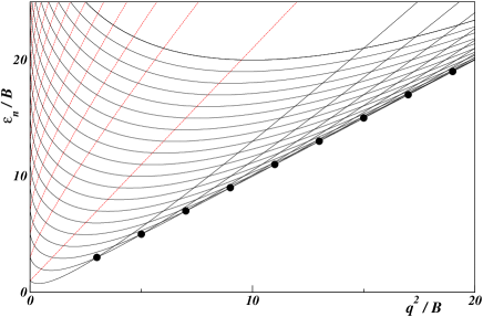
Figure 1: Energies of $\chi_{n+1}^{-}$ (black solid line) and $\chi_{n}^{+}$ (red dashed line) for $n=0,\dots,10$ as a function of $q^{2}/B$. The crossings of the ground–states occur in the degeneracy points $q^{2}/B=\left(1+2n\right)$, denoted by solid circles.

We notice that the angular momentum is not a good quantum number for this states unless we introduce also a spin–$1/2$ component defining a total angular momentum $J=L+S$. $J$ commutes with both the Hamiltonians (27) and (34) and $J\chi_{n,m}^{\pm}=\left(n-m-1/2\right)\chi_{n,m}^{\pm}$. Moreover, the wavefunctions $\chi_{n,m}^{\pm}$ are eigenstates for the operator $n=D^{\dagger}D+\sigma_{z}/2$ defined in (16): thus, they constitutes deformed Landau levels.

Analyzing the spectrum, we can notice that there is a correspondence between the usual Landau levels and the states $\chi$’s trombettoni10 : every Landau level is splitted into two parts corresponding to the states $\chi_{n-1}^{+}$ and $\chi_{n}^{-}$ and, in the case $q\to 0$, their energy becomes approximately $E_{n-1}\pm 4q^{2}n$. Therefore, for $q\to 0$ one recovers the usual Landau levels structure characterized by the (double) spin degeneracy as prescribed by the condition $\mathcal{P}$3. The non-Abelian term of the Hamiltonian removes this degeneracy through the coupling between the $\left(n-1\right)^{\rm th}$ level with spin up and the $n^{\rm th}$ with spin down. The deformed Landau levels for $q>0$ can be defined also considering the Landau gauge; in palmer11 it is shown that, in this case, the eigenstates are distinguished by the $Z_{2}$ symmetry obtained by the parity transformation $x\to-x$.

Varying the value of the parameter $q^{2}/B$, measuring the ratio of the Abelian and non-Abelian contribution in the gauge potential, the eigenvalues $\varepsilon_{n}^{\pm}$ show an interesting pattern of crossing points (see Fig. 2): each pair of eigenstates of the kind $\chi^{-}_{a}$ and $\chi^{-}_{b}$ becomes degenerate for

$$\frac{q^{2}}{B}=\frac{1}{2}\left(a+b+\sqrt{1+4ab}\right)$$ (74)

and the energy of the crossing is $\varepsilon_{c}\left(a,b\right)=\left(a+b\right)B$. Instead, a pair of different eigenstates of the kind $\chi^{+}_{a}$ and $\chi^{-}_{b}$ has a crossing only if $a<b$; in this case the degeneracy point is

$$\frac{q^{2}}{B}=\frac{1}{2}\left(a+b-\sqrt{1+4ab}\right):$$ (75)

also for these levels the corresponding energy is $\varepsilon_{c}\left(a,b\right)=\left(a+b\right)B$. Therefore all the energy level crossings are characterized by an integer energy in units of $B$.

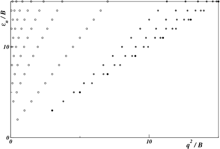
Figure 2: Crossing points of the eigenvalues: black (gray) circles indicate the crossings between states $\chi_{n+1}^{-}$ corresponding to the ground–state (excited states). Whereas circles denote the crossings of the states $\chi_{n+1}^{-}$ with the states $\chi_{n}^{+}$ ($n=0,\dots,10$). The coordinate $q^{2}/B$ for these degeneracy points are provided in Equations (74,75).

As shown in Fig. 1 the uncoupled state family (71), corresponding to $\chi_{0}^{+}$, is characterized by the energy $\varepsilon_{0}^{+}=B+2q^{2}$, which is higher than the energy $\varepsilon_{1}^{-}=2B+2q^{2}-\sqrt{B^{2}+8Bq^{2}}$ of $\chi_{1}^{-}$. Therefore $\chi_{1}^{-}$ is the ground–state family of the system for $q^{2}<3B$ (the general case with $q^{2}\geq 3B$ is analyzed in section V.1). We can rewrite each state of the family $\chi_{1}^{-}$ in the form

$$\chi_{1}^{-}=e^{-\frac{B}{4}\left|z\right|^{2}}\left(c_{\uparrow,1}P\left|\uparrow\right\rangle+2c_{\downarrow,1}B\bar{z}P\left|\downarrow\right\rangle-4c_{\downarrow,1}\partial_{z}P\left|\downarrow\right\rangle\right),$$ (76)

where $P$ is a generic polynomial in $z$ and we defined the constants

$$c_{\uparrow,n} = B+2q\sqrt{2Bn}+\sqrt{B^{2}+8q^{2}Bn}$$ (77)

$$c_{\downarrow,n} = i\left({B-2q\sqrt{2Bn}-\sqrt{B^{2}+8q^{2}Bn}}\right)\left(2\sqrt{2Bn}\right)^{-1}.$$ (78)

It is also convenient to introduce the operator

$$\mathcal{G}_{1}\equiv c_{\uparrow,1}\sigma_{x}+c_{\downarrow,1}d^{\dagger}$$ (79)

that allows us to map uncoupled states in $\chi_{0}^{+}$ in states in $\chi_{1}^{-}$ trombettoni10 . Thus, we can rewrite (76) using the operator $\mathcal{G}_{1}$

$$\chi_{1}^{-}=\mathcal{G}_{1}\left(P(z)e^{-\frac{B}{4}\left|z\right|^{2}}\left|\downarrow\right\rangle\right).$$ (80)

Due to the degeneracy of these ground–states, one can build also wavefunctions minimizing supplementary terms in the Hamiltonian (28); for instance, we can introduce a repulsive potential for the spin up component of the form $V_{\uparrow}\left(z,\zeta\right)=\delta\left(z-\zeta\right)\left|\uparrow\right\rangle\left\langle\uparrow\right|$ where $\zeta$ plays the role of the coordinates of a quasi–hole in the spin up wavefunction. The corresponding single–particle ground–states are

$$\phi\left(z,\zeta\right)=\mathcal{G}_{1}\left(\left(z-\zeta\right)Q\left(z\right)e^{-\frac{B}{4}\left|z\right|^{2}}\left|\downarrow\right\rangle\right)$$ (81)

where $Q(z)$ is a generic polynomial. We observe that the wavefuntion density for the spin up component in $\phi$ goes to zero for $z=\zeta$ while the spin down density, in general, does not, due to the derivative term in $d^{\dagger}$. We can also consider a repulsive potential not affected by the spin, $V\left(\zeta\right)=\delta\left(z-\zeta\right)$: in this case we obtain as a ground–state the wavefunctions

$$\Phi\left(z,\zeta\right)=\mathcal{G}_{1}\left(\left(z-\zeta\right)^{2}Q(z)e^{-\frac{B}{4}\left|z\right|^{2}}\left|\downarrow\right\rangle\right)$$ (82)

having a vanishing density in $\zeta$ both for the spin up and the spin down component. Notice that it is impossible to create inside the space $\chi_{1}^{-}$ a wavefunction with a zero spin–down density in $\zeta$ and a non-vanishing spin up component.

With respect to the Hamiltonian (27), these excitations are gapless; however they increase the total angular momentum of the system, and, as we will show in section VI, this implies an increment in energy once we consider the case $\Delta=\omega-\Omega\neq 0$ in (36).

IV.1 $U(3)$ non–Abelian gauge potentials

As shown in juze10 ; goldman11 , it is possible to engineer gauge potentials involving a higher number of internal states. For instance, considering atoms with a tetrapod electronic structure, one can obtain three degenerate dark states, which we denote by $\left|+\right\rangle$, $\left|0\right\rangle$ and $\left|-\right\rangle$: this corresponds to an effective spin 1 and it allows to mimic the effect of an external $U(3)$ non–Abelian gauge potential.

In particular we can generalize the construction of the previous Section to the following potential:

$$A_{x}=-\frac{B}{2}y\,\mathbb{I}+\begin{pmatrix}0&\alpha&0\\ \alpha&0&\beta\\ 0&\beta&0\end{pmatrix}\,,\qquad A_{y}=\frac{B}{2}x\,\mathbb{I}+\begin{pmatrix}0&-i\alpha&0\\ i\alpha&0&-i\beta\\ 0&i\beta&0\end{pmatrix}$$ (83)

where $\mathbb{I}$ is the $3\times 3$ identity matrix, $B$ is the effective magnetic field and $\alpha$ and $\beta$ are two arbitrary parameters giving the coefficients of different Gell-Mann matrices. $A_{x}$ and $A_{y}$ do not commute and they describe a particular family of effective homogeneous non-Abelian $U(3)$ potentials whose corresponding non-Abelian magnetic field is

$$\mathcal{B}=\begin{pmatrix}B-2\alpha^{2}&0&0\\ 0&B+2\alpha^{2}-2\beta^{2}&0\\ 0&0&B+2\beta^{2}\end{pmatrix}$$ (84)

which is translationally invariant as in Equation (29). These potentials are similar to the one chosen in goldman11 to simulate Weyl fermions through multi–component ultracold atoms in optical lattices.

Given the potential (83), the minimal coupling Hamiltonian assumes the form:

$$H\left(\alpha,\beta\right)=B+\frac{1}{4}d^{\dagger}d+\begin{pmatrix}2\alpha^{2}&-i\alpha d&0\\ i\alpha d^{\dagger}&2\alpha^{2}+2\beta^{2}&-i\beta d\\ 0&i\beta d^{\dagger}&2\beta^{2}\end{pmatrix}$$ (85)

where we used the operators $d$ and $d^{\dagger}$ defined in (64). The first term in $H\left(\alpha,\beta\right)$ is the Abelian term proportional to the identity, while the second one describes the non–Abelian interaction, depending on the parameters $\alpha$ and $\beta$, coupling subsequent Landau levels with different spin as in the $U(2)$ case. Therefore, for each $n\geq 2$, we can identify three families of eigenstates obtained by linear superpositions of the states $\psi_{n,m}\left|-\right\rangle$, $\psi_{n-1,m}\left|0\right\rangle$ and $\psi_{n-2,m}\left|+\right\rangle$, where $m$ is related to the angular momentum. In particular, given $n\geq 2$, the corresponding eigenenergies of $H\left(\alpha,\beta\right)$ are the solutions $\varepsilon_{n}$ of the following eigenvalues equation (see Fig. 3 for the case $\alpha=\beta$):

$$\begin{pmatrix}2\alpha^{2}+B\left(2n-3\right)&-i2\alpha\sqrt{2B\left(n-1\right)}&0\\ i2\alpha\sqrt{2B\left(n-1\right)}&2\alpha^{2}+2\beta^{2}+B\left(2n-1\right)&-i2\beta\sqrt{2Bn}\\ 0&i2\beta\sqrt{2Bn}&2\beta^{2}+B\left(2n+1\right)\end{pmatrix}=\varepsilon_{n}\mathbb{I}.$$ (86)

Like the case of the Jaynes–Cummings coupling, the spin degeneracy of the Landau levels is removed and the eigenstates of (85) are also eigenstates of the total angular momentum $J$.

In analogy with the previously discussed $U(2)$ potential, there are also other eigenstates of the Hamiltonian (85) corresponding to the uncoupled states $\psi_{0,m}\left|-\right\rangle$ with energy $\varepsilon_{0}=2\beta^{2}+B$ and to the family of (unnormalized) “doublet states” defined by

$$\Phi^{\pm}_{m}=\left(B-\alpha^{2}\mp\sqrt{\left(\alpha^{2}-B\right)^{2}+8B\beta^{2}}\right)\psi_{0,m}\left|0\right\rangle-i\beta\sqrt{8B}\psi_{1,m}\left|-\right\rangle$$ (87)

with energy

$$\varepsilon_{1}^{\pm}=2B+2\beta^{2}+\alpha^{2}\pm\sqrt{\left(\alpha^{2}-B\right)^{2}+8B\beta^{2}}.$$ (88)

We observe that in the limit $\alpha\to 0$ or $\beta\to 0$ the results of the previous Section are recovered. In fact, if either $\alpha$ or $\beta$ goes to zero, the resulting gauge potential is an effective $U(2)$ potential of the kind (27) and one of the spin states remains decoupled with respect to the others.

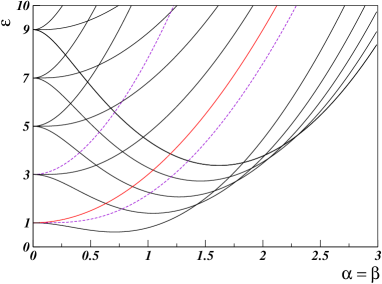
Figure 3: The energy levels of the Hamiltonian (85) are plotted imposing the constraint $\alpha=\beta$ (with $B=1$). The black lines represent the eigenvalues $\varepsilon_{n}$ (86), the purple dashed lines represent the energy $\varepsilon_{1}^{\pm}$ of the doublet states and the red line represents the energy $\varepsilon_{0}$ of the uncoupled states. One can see that, in the limit $\alpha=\beta\to 0$, the Landau level energies are recovered with a threefold pseudospin degeneracy.

Finally Fig. 4 shows that it is possible to recover a triple degeneracy of the ground–state for particular values of the parameters $\alpha$ and $\beta$. The figure shows a triple degeneracy occurring for $B=1$, $\alpha=\sqrt{\left(9+\sqrt{73}\right)/6}$ and $\beta=\sqrt{2/3}$ between the uncoupled state and two eigenvectors of (86) obtained for $n=2$ and $n=3$ at the energy $\varepsilon=\frac{7}{3}B$. We also checked that lines of doubly degenerate ground–states occur in the plane defined by $\alpha$, $\beta$ (single points with triple degeneracy belong of course to these lines). Further details on the spectrum of Hamiltonian (85) will be presented elsewhere.

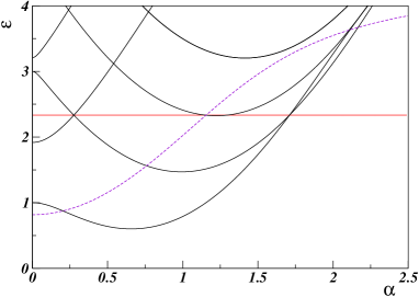
Figure 4: The first energy levels of the Hamiltonian (85) are plotted as a function of $\alpha$ for $\beta=\sqrt{2/3}$ and $B=1$. The black lines represent the eigenvalues $\varepsilon_{n}$ (86), the purple dashed line represents the energy $\varepsilon_{1}^{-}$ of the first doublet states and the red line represents the energy $\varepsilon_{0}=7/3$ of the uncoupled states. For this choice of the parameters a triple degeneracy of the ground states appear for $\alpha=\sqrt{\left(9+\sqrt{73}\right)/6}\simeq 1.71$.

V Two–body interactions and deformed Laughlin states

In the previous Section we described a single particle with two internal degrees of freedom in the non–Abelian potential (27): we consider in this Section a system of $N$ atoms, introducing two–body repulsive interactions. Denoting by $g_{1}$ the (dimensionless) scattering length between particles in the same internal state and by $g_{0}$ the scattering length between particles in different internal states, we can write the interaction Hamiltonian as

$$H_{I}=\sum\limits_{i<j}^{N}\left(g_{1}\Pi_{1}+g_{0}\Pi_{0}\right)\delta\left(z_{i}-z_{j}\right).$$ (89)

Here $\Pi_{1}$ is the projector over the space in which the particles $i$ and $j$ have parallel spin states ($\left|\uparrow\uparrow\right\rangle$ or $\left|\downarrow\downarrow\right\rangle$), whereas $\Pi_{0}$ is the projector over the space in which $i$ and $j$ have antiparallel spins ($\left|\uparrow\downarrow\right\rangle$ or $\left|\downarrow\uparrow\right\rangle$). We will consider both bosonic and fermionic gases, keeping in mind that for fermions it is $g_{1}=0$ pitaevskii03 ; pethick08 .

An arbitrary two–particle state in which both atoms are in $\chi_{1}^{-}$ can be described as

$$\Psi=\mathcal{G}_{1,1}\mathcal{G}_{1,2}P\left(z_{1},z_{2}\right)e^{-B\left(\left|z_{1}\right|^{2}+\left|z_{2}\right|^{2}\right)/4}\left|\downarrow\downarrow\right\rangle,$$ (90)

where $\mathcal{G}_{1,i}$, defined in (79), refers to the coordinate $z_{i}$, and $P$ is generic polynomial in $z_{1}$ and $z_{2}$. With vanishing inter–species interaction ($g_{0}=0$) and strong intra–species interaction, $\Psi$ has a zero interaction energy if its components $\left|\uparrow\uparrow\right\rangle$ , $\left|\downarrow\downarrow\right\rangle$ vanish when $z_{1}\to z_{2}$: for fermions, this is assured by the Pauli principle; whereas for bosons the strong intra-species regime corresponds to $g_{1}\gg B,q$ and the two–body wavefunction $\Psi$ has to fulfil the requirements

$$P\left(z,z\right)=0\,,\quad\left.\left(\partial_{z_{1}}+\partial_{z_{2}}\right)P\right|_{z_{1}=z_{2}}=0\,,\quad\left.\partial_{z_{1}}\partial_{z_{2}}P\right|_{z_{1}=z_{2}}=0.$$ (91)

Every antisymmetric polynomial $P\left(z_{1},z_{2}\right)=-P\left(z_{2},z_{1}\right)$ obviously satisfies these constraints, and, in general, all the fermionic functions $\Psi\left(z_{1},z_{2}\right)$ guarantee that the intra–species interaction gives a zero energy contribution.

If we add also an inter–species repulsive interaction, such that $g_{0}\gg B,q$, the two–particle wavefunction (90) must satisfy the further constraints

$$\left.\partial_{z_{1}}P\right|_{z_{1}=z_{2}}=\left.\partial_{z_{2}}P\right|_{z_{1}=z_{2}}=0$$ (92)

in order to be a ground–state of $H_{I}$. These relations hold, for instance, in the case $P=\left(z_{1}-z_{2}\right)^{m}$ with $m>1$. In the case $m=2$ the inter–species interaction is zero, but not the intra–species one, whereas for $m\geq 3$ every repulsive potential $H_{I}$ gives a null contribution. In the following we consider the regime given by $g_{0}=0$ and (for bosons) $g_{1}\gg B>3q^{2}$. Under these conditions we can generalize the previous results for the case of $N$ atoms.

The fermionic states, antisymmetric by the exchange of every pair of atoms, have a zero interaction energy; thus, a possible ground–state of the $N$–particle Hamiltonian $\mathcal{H}=\sum_{k=1}^{N}H_{k}+H_{I}$, with all the atoms in the $\chi_{1}^{-}$ space in order to minimize the single–particle energy, is given by

$$\Psi=\left[{\prod\limits_{i}^{N}\mathcal{G}_{1,i}}\right]\left(\mathcal{A}\left[P_{0}\left(z_{1}\right),...\,,P_{N-1}\left(z_{N}\right)\right]e^{-\frac{B}{4}\sum\limits_{i}^{N}\left|z_{i}\right|^{2}}\left|\downarrow\downarrow...\downarrow\right\rangle\right),$$ (93)

where $\mathcal{A}$ is the antisymmetrization over all the coordinates $z_{i}$ and $P_{m}$ are different polynomials. Generalizing this kind of many-body states, it is easy to define a deformation, due to the non–Abelian potential, of the common Laughlin states. If we choose $P_{m}(z)=z^{m}$ with $m=0,...,N-1$, we obtain the usual Jastrow factor $\mathcal{A}\left[P_{0}...P_{N-1}\right]=\prod_{i<j}^{N}\left(z_{i}-z_{j}\right)$. More in general, given a Laughlin wavefunction

$$\Lambda_{N}^{(m)}=\prod\limits_{i<j}^{N}\left(z_{i}-z_{j}\right)^{m}e^{-\frac{B}{4}\sum\limits_{i}^{N}\left|z_{i}\right|^{2}}\left|\downarrow\downarrow...\downarrow\right\rangle$$ (94)

with $m$ odd, the state

$$\Psi^{(m)}=\prod\limits_{j}^{N}\mathcal{G}_{1,j}\Lambda_{N}^{(m)}$$ (95)

is a ground–state of the Hamiltonian $\mathcal{H}$: every atom lies in a superposition of states $\chi_{1}^{-}$ and the antisymmetric wavefunction causes the intra–species interaction energy to be zero.

Also for bosons, symmetric under the exchange of two particles, there are states that have a zero intra-species interaction. For instance we can consider $\Psi^{(m)}$ for an even value of $m\geq 4$. In this case for each pair of particles with $z_{i}\to z_{j}$ the wavefunction vanishes at least as $\left(z_{i}-z_{j}\right)^{2}$, thus the interaction energy (and also its inter–species contribution if $g_{0}\neq 0$) is vanishing.

Therefore it is important to notice that the introduction of the non–Abelian gauge potential (in the regime $q^{2}<3B$) implies that the highest density deformed Laughlin state with null interaction energy has a filling factor $1/4$ instead of the usual filling factor $1/2$ that characterizes systems of rotating bosons cooper08 ; cooper05 with a contact interaction. Thus we expect that the introduction of the $SU(2)$ potential gives rise to the incompressible state $\Psi^{(4)}$, as numerically observed for small values of the chemical potential in the weak-interacting regime palmer11 . Such state is absent in the case of a pure magnetic field and it can be considered as a signature of the effect of the potential (27).

The state $\Psi^{(m)}$ describes in general an incompressible fluid of spin–$1/2$ particles, as it can be shown calculating its norm: one finds

$$I=\left\langle\Psi^{(m)}|\Psi^{(m)}\right\rangle=\left\langle\Lambda_{N}^{(m)}\right|\prod\mathcal{G}_{1,j}^{\dagger}\mathcal{G}_{1,j}\left|\Lambda_{N}^{(m)}\right\rangle=\\ =\left\langle\Lambda_{N}^{(m)}\right|\prod\limits_{j}^{N}\left(\left|c_{\uparrow,1}\right|^{2}+\left|c_{\downarrow,1}\right|^{2}d_{j}d_{j}^{\dagger}+\sigma_{x,j}\left(c_{\uparrow,1}^{*}c_{\downarrow,1}d_{j}^{\dagger}+c_{\uparrow,1}c_{\downarrow,1}^{*}d_{j}\right)\right)\left|\Lambda_{N}^{(m)}\right\rangle=\\ =\left(\left|c_{\uparrow,1}\right|^{2}+8B\left|c_{\downarrow,1}\right|^{2}\right)^{N}\left\langle\Lambda_{N}^{(m)}|\Lambda_{N}^{(m)}\right\rangle,$$ (96)

where we considered that all the single–particle states involved in $\Psi^{(m)}$ are in the lowest Landau level and therefore are eigenstates of $dd^{\dagger}$. Thus the norm $I$ can be easily written in terms of the one of the Laughlin state, and one can apply the argument also to $\Psi^{(m)}$.

This is true also if we consider quasi–holes in the Laughlin state as, for example

$$\Psi_{\zeta_{1},\zeta_{2}}^{(m,k)}=\prod\limits_{i}^{N}\mathcal{G}_{1,i}\left(\prod\limits_{i}^{N}\left(z_{i}-\zeta_{1}\right)^{k}\left(z_{i}-\zeta_{2}\right)^{k}\right)\Lambda_{N}^{(m)},$$ (97)

since each atom in the Laughlin state is in the lowest Landau level, and thus the operators $\mathcal{G}_{1}$ modify only the norm of the states by a constant factor for each atom.

This correspondence highlights the nature of these excitations since it allows us to state that the Berry phase due to the adiabatic exchange of the pair of quasi–holes $\zeta_{1}$ and $\zeta_{2}$ is the same of the one characterizing the corresponding quasi–holes in a simple Laughlin state. This kind of excitations are therefore Abelian anyons and their braiding statistics is ruled by the usual exchange properties of the Abelian states in the fractional quantum Hall effect arovas84 .

V.1 Generalization to higher value of $q^{2}/B$

So far we referred to the case $q^{2}<3B$ in which the ground–state family is provided by wavefunctions of the kind $\chi^{-}_{1}$. However, as shown in Fig. 1, for higher values of $q$ different ground–states families alternate. Therefore it is necessary to generalize the previous results also for $q^{2}\geq 3B$ by defining the family of operators $\mathcal{G}_{n}$ describing the deformed Landau levels of the kind $\chi^{-}$. From (74) one sees that $\chi_{n>1}^{-}$ is the ground–state family for

$$\left(2n-1\right)B<q^{2}<\left(2n+1\right)B:$$ (98)

its energy $\varepsilon_{n}^{-}$ varies, in this range of $q$, from $\left(2n-1\right)B$ to $\left(2n+1\right)B$. To describe the ground–state family $\chi_{n}^{-}$ we generalize the operator $\mathcal{G}_{1}$ (79) introducing the operators

$$\mathcal{G}_{n}=c_{\uparrow,n}\,d^{{\dagger}\,(n-1)}\sigma_{x}+c_{\downarrow,n}\,d^{{\dagger}\,n},$$ (99)

where the constants $c_{\uparrow,n}$ and $c_{\downarrow,n}$ are defined in (77,78). The ground–state wavefunctions can be expressed in the form

$$\chi_{n}^{-}=\mathcal{G}_{n}\left(P(z)e^{-\frac{B}{4}\left|z\right|^{2}}\left|\downarrow\right\rangle\right).$$ (100)

Using these expressions and following the procedure shown in the case of $\chi_{1}^{-}$, it is possible to obtain the appropriate many–body wavefunctions for each value of $B$ and $q$, with $n$ chosen in order to satisfy (98) (the case of the degeneracy points $q^{2}=\left(2n+1\right)B$ will be analyzed in section VII). In particular, for an arbitrary $n$, all the antisymmetric states given by

$$\Psi_{n}^{(m)}=\prod\limits_{j}^{N}\mathcal{G}_{n,j}\Lambda_{N}^{(m)},$$ (101)

with $\Lambda_{N}^{(m)}$ an odd Laughlin state (94), are fermionic ground–states unaffected by repulsive intra–species contact interactions (here $\mathcal{G}_{n,j}$ indicates the operator $\mathcal{G}_{n}$ applied to the atom $j$).

For bosons having repulsive delta interactions (both intra–species and inter–species) one has to consider the derivatives present in the operators $\mathcal{G}_{n}$ to find a ground–state having zero interaction energy. The highest order derivative in $\mathcal{G}_{n}$ is given by the term $\partial_{z}^{n}$ in the $\left|\downarrow\right\rangle$ component of each particle. Therefore, to identify the smallest even power $m$ in (101) annihilating a delta interaction, one has to consider for each pair of particles the $\left|\downarrow\downarrow\right\rangle$ component: in order to make the repulsive delta interaction null there must be a factor $\left(z_{i}-z_{j}\right)^{m}$ with $m>2n$. Once the polynomial order of the wavefunction (101) is high enough to make vanish the interaction in the $\left|\downarrow\downarrow\right\rangle$ component, then also all the other components give a null contribution. Therefore the bosonic wavefunction $\Psi_{n}^{(2n+2)}$ is the ground–state with the smallest polynomial order for generic repulsive delta interaction.

As a consequence, $\Psi_{n}^{(2n+2)}$ defines the maximum filling factor $\nu_{n}=1/\left(2n+2\right)$ over which the interaction energy among bosons cannot be zero. In the range (98) only states with $\nu<1/\left(2n+2\right)$ can have a null interaction energy for $z_{i}\to z_{j}$ in the $\left|\downarrow\downarrow\right\rangle_{ij}$ component. This result is consistent with the numerical data obtained in palmer11 where it is shown that, in the case of $q^{2}<3B$, the Laughlin state with $\nu=1/2$ has a positive interaction energy, whereas for $\nu=1/4$ the energy is exactly zero. In this regime, in fact, $m$ must be at least $4$ to give a true ground–state, as already observed in the previous Section. Moreover, the maximum filling factor $\nu_{n}$ decreases as $q^{2}/B$ increases, therefore the role of interactions becomes more and more important if we consider higher filling factors for high values of $q$. This could explain why, for $\nu>1/2>\nu_{n}$, there are no numerical evidences of incompressible bosonic states after the first Landau level crossing ($q^{2}>3B$) palmer11 .

VI The effect of angular momentum

As mentioned in Section III, the single–particle Hamiltonian (28) can be considered as the limit of the Hamiltonian $H_{L}$ (36) when the angular velocity $\Omega$ approaches the trapping frequency $\omega$. However, so far we considered only cases in which the condition $\mathcal{P}$2 in Section II.3 holds and we neglected an eventual energy contribution of the angular momentum. In this Section we analyze the effect of the angular momentum term in the Hamiltonian (36) in order to calculate the energy of the states $\Psi_{n}^{(m)}$ (and their excitations) and to determine the constraints which $\Delta=\omega-\Omega$ must satisfy not to spoil the Landau level description.

Let us consider the single–particle Hamiltonian (36):

$$H_{L}=\left(\vec{p}+\vec{A}\right)^{2}-\Delta L_{z}.$$

The term proportional to $\Delta$ is spin–independent and it does not affect the non-Abelian contribution $H_{na}$ in (63). Using its eigenstates $\varphi_{n,m}^{\pm}$ (67) for $n\geq 1$ we can split $H_{L}$ into blocks of the form

$$H_{L,n,m}=2q^{2}+2Bn-\Delta\left(n-m-\frac{1}{2}\right)+\begin{pmatrix}2q\sqrt{2Bn}&-B+\frac{\Delta}{2}\\ -B+\frac{\Delta}{2}&-2q\sqrt{2Bn}\end{pmatrix}.$$

The eigenenergies of $H_{L}$ are therefore

$$\varepsilon_{n,m}^{\pm}=2Bn+2q^{2}-\Delta\left(n-m-\frac{1}{2}\right)\pm\sqrt{\left(B-\frac{\Delta}{2}\right)^{2}+8q^{2}Bn}$$ (102)

and the corresponding (unnormalized) eigenstates are

$$\chi_{n,m}^{\pm}=\left(B-\frac{\Delta}{2}+2q\sqrt{2Bn}\mp\sqrt{\left(B-\frac{\Delta}{2}\right)^{2}+8q^{2}Bn}\right)\psi_{n-1,m}\left|\uparrow\right\rangle+\\ +\left(B-\frac{\Delta}{2}-2q\sqrt{2Bn}\pm\sqrt{\left(B-\frac{\Delta}{2}\right)^{2}+8q^{2}Bn}\right)\psi_{n,m}\left|\downarrow\right\rangle.$$ (103)

We see that the uncoupled eigenstates are unaffected by the angular momentum term.

Since the coefficients in the definition of the eigenstates do not depend on $m$, then one can redefine the constants $c_{\uparrow,n}$, $c_{\downarrow,n}$ and the operators $\mathcal{G}_{n}$ independently on $m$. Moreover, the Landau level structure holds also for $H_{L}$ (condition $\mathcal{P}$1), and the Landau levels are energetically distinguishable provided that the energy contribution of the angular momentum remains small with respect to the Landau level spacing. In fact, all the energy levels (102) have a term which is linear in the total angular momentum $J=n-m-1/2$ (increasing their energy if $J<0$). Thus the states with lower values of $m$ are favoured: this implies an energy gap $\Delta$ for the creation of single–particle quasi–holes of the kind (81) and $2\Delta$ for (82) (for $\zeta=0$).

In order to understand the stability of the Landau level structure, and thus of the deformed Laughlin states, we have to consider a multiparticle wavefunction describing $N$ atoms in a ground–state of the kind $\Psi_{n}^{(m)}$ (101) for $2n-1<q^{2}/B<2n+1$. In this case a particle corresponding to the highest value of the modulus of the angular momentum term $\left|J\right|$ acquires an additional energy $\sim Nm\Delta$ that must be smaller than the gap with the next deformed Landau level. This gap, for values of $q^{2}$ far from the degeneracy points, can be calculated evaluating the energy difference of $\chi^{-}_{n}$ and $\chi^{-}_{n-1}$ in the crossing point between $\chi^{-}_{n-1}$ and $\chi^{-}_{n+1}$ and it can be approximated by $B/(2n)$. Therefore the Landau level description of the multiparticle states remains accurate if $\Delta\ll B/(2nNm)$.

Let us analyze more in detail the regime characterized by small values of $\Delta$. The deformed Laughlin states $\Psi_{n}^{(m)}$ have to be defined with the appropriate corrections in the operators $\mathcal{G}_{n}$ (99) since the constants $c_{\uparrow}$ and $c_{\downarrow}$ must include $\Delta$ coherently with (103). The corresponding energy contribution of the total angular momentum turns to be for $\Psi_{n}^{(m)}$

$$-\Delta J\Psi_{n}^{(m)}=\Delta N\left(\frac{mN}{2}-m-n+\frac{1}{2}\right)\Psi_{n}^{(m)}\approx\Delta m\frac{N^{2}}{2}\Psi_{n}^{(m)}.$$ (104)

Therefore, the Laughlin states with smaller $m$ (and higher density) are energetically favoured: thus, in the case of fermions, far from the degeneracy points, the ground–states are described by the $\nu=1$ filling factor states $\Psi_{n}^{1}$, whereas in the case of bosons the ground–states are of the form $\Psi_{n}^{2n+2}$.

A quasi–hole in the position $\zeta=0$

$$\Psi_{n}^{(m)}=\prod\limits_{j}^{N}\mathcal{G}_{n,j}\prod\limits_{j}^{N}z_{j}^{k}\Lambda_{N}^{(m)}$$ (105)

acquires an additional energy $N\Delta k$ with respect to the corresponding ground–state, because it changes the angular momentum of each particle by $k$. This energy can be considered the gap for the creation of a quasi–hole.

VII Degeneracy points and non–Abelian anyons

An important property of the single–particle spectrum of the Hamiltonian (28) is the existence of degeneracy points corresponding to the values $q^{2}=\left(1+2n\right)B$: this makes possible the occurrence of many–particle ground–states having non–Abelian excitations trombettoni10 . In these degeneracy points the two lowest energy levels cross (possibly generating a first-order phase transition palmer11 ) and the ground–state degeneracy of the single–particle is doubled. In these points an atom in the (non–interacting) ground–state can be described by all the superpositions of wavefunctions in $\chi_{n}^{-}$ and $\chi_{n+1}^{-}$. However, if we consider the angular momentum term in the Hamiltonian (see the previous Section), then the states with a lower angular energy are favoured and the variation of the parameter $q$ around the degeneracy points gives rise to a crossover, as we will describe in VII.3.

When the intra–species interaction between atoms is introduced, the doubled degeneracy of the single–particle states implies a novel form of the multiparticle ground–state which is quite different from (93,95). We first consider the case of the first degeneracy point, $q^{2}=3B$, in which there is the crossing between a ground–state of particles in $\chi_{1}^{-}$ and $\chi_{2}^{-}$ (our conclusions will be later extended to all the other degeneracy points). For the single particle the basis of ground–states is defined by the set $\left\{\mathcal{G}_{1}z^{m}\psi_{0}\left(z\right),\mathcal{G}_{2}z^{m}\psi_{0}\left(z\right),\;{\rm with}\;m\in\mathbb{N}\right\}$ and, analogously to the previous sections, we have to distinguish the case of interacting bosons and the one of (free) fermions.

VII.1 Fermionic gases

We first analyze the fermionic case: the highest density ground–state function of the Hamiltonian $\mathcal{H}$ for $2N$ atoms is given by trombettoni10

$$\Omega_{c}=\mathcal{A}\left[\mathcal{G}_{1}\psi_{0},\mathcal{G}_{1}z\psi_{0},...\,,\mathcal{G}_{1}z^{N-1}\psi_{0},\,\mathcal{G}_{2}\psi_{0},\mathcal{G}_{2}z\psi_{0},...\,,\mathcal{G}_{2}z^{N-1}\psi_{0}\right]\left|\downarrow\downarrow...\downarrow\right\rangle,$$ (106)

where $\mathcal{A}$ implements the full antisymmetrization over all the atoms. Because of the double degeneracy, the wavefunction $\Omega_{c}$ describes an atomic gas with filling factor $\nu=2$. The state $\Omega_{c}$ is obtained through the Slater determinant of the single–particle wavefunctions with the lowest angular momenta $\left|J\right|$, up to the power $z^{N-1}$. Therefore, considering also the angular momentum contribution in the Hamiltonian, it is the true ground–state for the system.

The double degeneracy makes $\Omega_{c}$ very different from the case (93): in the degeneracy points the antisymmetrization hides a clustering of the particles into two sets of $N$ atoms, say $A$ and $B$, that are physically different and refer to states in $\chi_{1}^{-}$ and in $\chi_{2}^{-}$. The two clusters must have the same number of atoms in order to minimize the contribution to the energy given by the angular momentum. The previous wavefunction can be recast in the form

$$\Omega_{c}=\mathcal{A}\left[\prod\limits_{k\in A}\mathcal{G}_{1,k}\prod\limits_{i<j\in A}\left(z_{i}-z_{j}\right)\prod\limits_{l\in B}\mathcal{G}_{2,l}\prod\limits_{i<j\in B}\left(z_{i}-z_{j}\right)\right]e^{-\frac{B}{4}\sum\limits_{i}^{2N}\left|z_{i}\right|^{2}}\left|\downarrow\downarrow...\downarrow\right\rangle$$ (107)

where we made explicit the Jastrow factor in each cluster and $\mathcal{A}$ refers to the antisymmetrization over all the possible clusterings in the sets $A$ and $B$. In the spirit of the quantum Hall states showing a clustering into two sets - the main example being the Moore and Read (MR) Pfaffian state moore91 ; nayak96 - $\Omega_{c}$ is characterized by the presence of quasi–hole excitations corresponding to half a quantum flux (and effective charge $1$, since $\nu=2$). These excitations must appear in pairs: it is however helpful to analyze the two possible wavefunctions they can assume. Such wavefunctions are related to quasi–holes in the two different clusters, given by

$$\sigma_{1}\left(\zeta\right)=\mathcal{A}\left[\prod\limits_{A}\mathcal{G}_{1,k}\prod\limits_{A}\left(z_{i}-z_{j}\right)\prod\limits_{A}\left(z_{i}-\zeta\right)\prod\limits_{B}\mathcal{G}_{2,l}\prod\limits_{B}\left(z_{i}-z_{j}\right)\right]e^{-\frac{B}{4}\sum\limits_{i}^{2N}\left|z_{i}\right|^{2}}\left|\downarrow...\downarrow\right\rangle$$ (108)

$$\sigma_{2}\left(\zeta\right)=\mathcal{A}\left[\prod\limits_{A}\mathcal{G}_{1,k}\prod\limits_{A}\left(z_{i}-z_{j}\right)\prod\limits_{B}\mathcal{G}_{2,l}\prod\limits_{B}\left(z_{i}-z_{j}\right)\prod\limits_{B}\left(z_{i}-\zeta\right)\right]e^{-\frac{B}{4}\sum\limits_{i}^{2N}\left|z_{i}\right|^{2}}\left|\downarrow...\downarrow\right\rangle.$$ (109)

These quasi–holes obey a fermionic statistics: once two of them of the same kind are exchanged, the wavefunction acquires a $\pi$ phase. However, it is interesting to notice that they show the same fusion rules of the Ising model with defined fermionic parity georgiev09 (characterizing the MR state moore91 ; nayak96 ) once one defines a third bosonic excitation given by the fusion $\psi\equiv\sigma_{1}\times\sigma_{2}$. From the physical point of view, if it is possible to obtain linear superpositions of $\sigma_{1}$ and $\sigma_{2}$ through the interplay between repulsive potentials for the $\left|\uparrow\right\rangle$ and $\left|\downarrow\right\rangle$ components, then the so–obtained (non–Abelian) excitations could present interesting features, a point which certainly deserves further investigations.

In fermionic systems at the degeneracy point $q^{2}=3B$, the ground–state $\Omega_{c}$, characterized by the filling factor $\nu=2$, is the highest density state obtained with atoms in the Hilbert space spanned by the deformed Landau level $\chi_{1}^{-}$ and $\chi_{2}^{-}$. Moreover, $\Omega_{c}$ minimizes the term in the Hamiltonian proportional to the angular momentum. Nevertheless, in the study of rotating ultracold atomic gases, it is interesting to analyze what happens varying the filling factor, since, in general, such systems present non-trivial phase diagrams as a function of $\nu$ cooper01 ; cooper05 ; cooper08 . As we have already shown, the double degeneracy at this particular value of $q^{2}$ provides in a natural way a clustering of the atoms into two sets in order to minimize $\left|J\right|$. Each atom can assume a wavefunction which is a superposition of states in $\chi_{1}^{-}$ and in $\chi_{2}^{-}$ and transitions from one to the other are possible: therefore, also for smaller values of the filling factor, we are driven to consider deformed ground–states showing a pairing among tha atoms that are similar to the ones usually considered in the study of fractional quantum Hall effect readgreen .

Let us consider first the filling factor $\nu=1$: in this case a paired state is built by favouring the creation of coupled atoms in the antisymmetric state obtained by applying the operator $\left(\mathcal{G}_{1,i}\mathcal{G}_{2,j}-\mathcal{G}_{2,i}\mathcal{G}_{1,j}\right)$ to the pair of atoms $(i,j)$ in the limit $z_{i}\to z_{j}$. The corresponding wavefunction for $2N$ particles reads

$$\Omega_{\rm Hf}={\rm Hf}\left(\left(\mathcal{G}_{1,i}\mathcal{G}_{2,j}-G_{2,i}G_{1,j}\right)\frac{1}{z_{i}-z_{j}}\right)\prod\limits_{i<j}^{2N}\left(z_{i}-z_{j}\right)e^{-\frac{B}{4}\sum\limits_{i}^{2N}\left|z_{i}\right|^{2}}\left|\downarrow\downarrow...\downarrow\right\rangle$$ (110)

where $\rm Hf$ indicates the Haffnian, which is a symmetric version of the Pfaffian defined for a symmetric matrix $M_{ij}=M_{ji}$:

$${\rm Hf}\left(M\right)=\sum\limits_{\sigma\in\mathcal{P}}M_{\sigma(1),\sigma(2)}M_{\sigma(3),\sigma(4)}...M_{\sigma(2N-1),\sigma(2N)}$$ (111)

(the sum is over all the permutation of the indices).

The wavefunction $\Omega_{\rm Hf}$ is antisymmetric over all the atoms because it is composed by the symmetric Haffnian and by the antisymmetric Jastrow factor. This implies that intra–species interactions give a zero contribution to the energy and $\Omega_{\rm Hf}$ can be considered a ground–state since each atom lies in a superposition of states of $\chi_{1}^{-}$ and $\chi_{2}^{-}$. However this wavefunction is not vanishing for $z_{i}\to z_{j}$ because of the components with different spin, therefore $\Omega_{\rm Hf}$ is not in general a ground–state for inter–species repulsive interactions that require higher powers of the Jastrow factor to give a null contribution.

For $\nu=1/2$ there are two possible antisymmetric paired states that have been widely analyzed in the literature. The first one corresponds to a deformed MR Pfaffian state moore91 ; nayak96 and the second corresponds to a deformed Haldane-Rezayi state haldane ; moore91 . The deformed MR Pfaffian state can be described by an effective $p$-wave pairing readgreen obtained by applying the operator $\left(\mathcal{G}_{1,i}\mathcal{G}_{2,j}+\mathcal{G}_{2,i}\mathcal{G}_{1,j}\right)$ which favours a symmetric state (with respect to $\chi_{1}^{-}$ and $\chi_{2}^{-}$) for the pair $(i,j)$ when $z_{i}\to z_{j}$. The corresponding wavefunction is trombettoni10

$$\Omega_{MR}={\rm Pf}\left(\left(\mathcal{G}_{1,i}\mathcal{G}_{2,j}+\mathcal{G}_{2,i}\mathcal{G}_{1,j}\right)\frac{1}{z_{i}-z_{j}}\right)\prod\limits_{i<j}^{2N}\left(z_{i}-z_{j}\right)^{2}e^{-\frac{B}{4}\sum\limits_{i}^{2N}\left|z_{i}\right|^{2}}\left|\downarrow\downarrow...\downarrow\right\rangle$$ (112)

where $\rm Pf$ is the Pfaffian operator. This wavefunction is antisymmetric, therefore intra–species interactions give a null contribution and $\Omega_{MR}$ can be considered a ground–state since each atom lies in a superposition of states in $\chi_{1}^{-}$ and $\chi_{2}^{-}$. This state shares all the main characteristics of the Moore and Read wavefunctions moore91 , and, in particular, its excitations are non–Abelian Ising anyons, as shown in nayak96 where an analogous wavefunction is analyzed. $\Omega_{MR}$ can be mapped into the usual spinless MR state $\Psi_{MR}$ moore91 ; nayak96 in a way which is similar to equation (95) for the ground–state outside the degeneracy points. Since, for every factor in the Pfaffian, one atom is in a state in $\chi^{-}_{1}$ and the other in $\chi^{-}_{2}$, the norm of $\Omega_{MR}$ is obtained from the one of the Pfaffian state $\Psi_{MR}$ just by multiplying it by a constant value for each pair of atoms:

$$\left\langle\Omega_{MR}\right|\left.\Omega_{MR}\right\rangle=\left(\left|c_{\uparrow,1}\right|^{2}+8B\left|c_{\downarrow,1}\right|^{2}\right)^{N}\left(8B\left|c_{\uparrow,2}\right|^{2}+2(8B)^{2}\left|c_{\downarrow,2}\right|^{2}\right)^{N}\left\langle\Psi_{MR}\right|\left.\Psi_{MR}\right\rangle.$$ (113)

This constant value can be calculated in a way similar to equation (96) and it is an effect of the clustering characterizing the state $\Omega_{MR}$. Equation (113) guarantees that also the statistics of the excitations $\zeta_{a}$ and $\zeta_{b}$ of the kind

$$\Omega_{MR}\left(\zeta_{a},\zeta_{b}\right)={\rm Pf}\left(\frac{\mathcal{G}_{1,i}\mathcal{G}_{2,i}\left(z_{i}-\zeta_{a}\right)\left(z_{j}-\zeta_{b}\right)+i\leftrightarrow j}{z_{i}-z_{j}}\right)\prod\limits_{i<j}^{2N}\left(z_{i}-z_{j}\right)^{2}e^{-\frac{B}{4}\sum\limits_{i}^{2N}\left|z_{i}\right|^{2}}\left|\downarrow\downarrow...\downarrow\right\rangle$$ (114)

can be described by Ising anyons as in the case of the Moore and Read state, since the Berry and monodromy phases acquired in the exchange of two excitations coincide.

The other paired ground–state at $\nu=1/2$ is a deformed Haldane-Rezayi state that can be obtained through the introduction of the antisymmetric operator $\left(\mathcal{G}_{1,i}\mathcal{G}_{2,j}-\mathcal{G}_{2,i}\mathcal{G}_{1,j}\right)$:

$$\Omega_{HR}={\rm Pf}\left(\left(\mathcal{G}_{1,i}\mathcal{G}_{2,j}-\mathcal{G}_{2,i}\mathcal{G}_{1,j}\right)\frac{1}{\left(z_{i}-z_{j}\right)^{2}}\right)\prod\limits_{i<j}^{2N}\left(z_{i}-z_{j}\right)^{2}e^{-\frac{B}{4}\sum\limits_{i}^{2N}\left|z_{i}\right|^{2}}\left|\downarrow\downarrow...\downarrow\right\rangle.$$ (115)

This state has a total angular momentum $\left|J\right|$ which is lower than the one of $\Omega_{MR}$ so that, in principle, it is energetically favoured if we consider the single-particle Hamiltonian (36). However the Haldane-Rezayi state represents the critical point between a weak and a strong coupling phase in a fermionic system with an effective $d$-wave pairing readgreen , therefore it is considered to be a gapless state whose excitations are described by a non–unitary conformal field theory gurarie which is unfit to define an incompressible state. Moreover we expect that $\Omega_{HR}$ is more influenced by the presence of a weak inter–species interaction than $\Omega_{MR}$.

To conclude the discussion about the (free) fermionic gases it is worth noticing that all the states presented can be retrieved also for the generic degeneracy point between states in $\chi^{-}_{n}$ and $\chi^{-}_{n+1}$ by substituting the operators $\mathcal{G}_{1}$ and $\mathcal{G}_{2}$ with $\mathcal{G}_{n}$ and $\mathcal{G}_{n+1}$. This is true in the case of free fermions (i.e., with $g_{0}=0$), whereas the introduction of strong interactions, such as an inter–species contact repulsion, brings to different scenarios presenting deformed Halperin states, similar to the one we will present for the bosonic gases, whose exponents and filling factors depend also on the value of $n$.

VII.2 Bosonic gases

The analysis of the degenerate points can be applied also to bosonic gases. As described in Section V.1, the state $\Psi^{(m)}_{n}$ (101) is a ground–state of both the intra–species and the inter–species contact interactions for every $m>2n$, therefore $\Psi^{(2n+2)}_{n}$ is the bosonic wavefunction with zero interaction energy minimizing the polynomial order. In the point $q^{2}=3B$ one has a superposition of states in $\chi_{1}^{-}$ and in $\chi_{2}^{-}$ and, as in the previous case, we can describe the related multiparticle ground–state through the clustering in two corresponding subsets $A$ and $B$. The resulting ground–state is

$$\Omega_{b}=\mathcal{S}\left[\prod\limits_{k\in A}\mathcal{G}_{1,k}\prod\limits_{i<j\in A}\left(z_{i}-z_{j}\right)^{4}\prod\limits_{l\in B}\mathcal{G}_{2,l}\prod\limits_{i<j\in B}\left(z_{i}-z_{j}\right)^{6}\prod\limits_{k\in A,l\in B}\left(z_{k}-z_{l}\right)^{4}\right]e^{-\frac{B}{4}\sum\limits_{i}^{2N}\left|z_{i}\right|^{2}}\left|\downarrow\downarrow...\downarrow\right\rangle=\\ =\mathcal{S}\left[\prod\limits_{k\in A}\mathcal{G}_{1,k}\prod\limits_{l\in B}\mathcal{G}_{2,l}\prod\limits_{i<j\in B}\left(z_{i}-z_{j}\right)^{2}\right]\Lambda^{(4)}_{2N}$$ (116)

where the symmetrization over all the atoms is necessary to have a bosonic state and $\Lambda^{(4)}$ is the generalized Laughlin state (94). The exponents of the Jastrow factors are defined considering that the lowest polynomial order term for an atom in $A$ is given by the first derivative included in $\mathcal{G}_{1}$, whereas in $B$ by the second derivative in $\mathcal{G}_{2}$. Therefore $\Omega_{b}$ vanishes at least as $\left(z_{i}-z_{j}\right)$ whenever $z_{i}\to z_{j}$ for each pair of atoms, and the intra–species interaction energy is zero. $\Omega_{b}$ is characterized by a filling factor $\nu=2/9$ and it is built by the symmetrization of the Halperin state $\Psi\left(4,6,4\right)$. The interaction term between atoms in different clusters is determined in order to satisfy the zero interaction energy constraint

$$\prod\limits_{k\in A,l\in B}\partial_{z_{k}}\partial^{2}_{z_{l}}\left(z_{k}-z_{l}\right)^{4}\propto\left(z_{k}-z_{l}\right).$$

The $\Omega_{b}$ filling factor, $\nu=2/9$, is therefore the highest possible filling factor that guarantees a null interaction energy for bosons at the point $q^{2}=3B$.

We conclude this Section observing that considering different degeneracy points, $q^{2}=(2n+1)B$, the ground states for intra–species repulsions are defined as deformed Halperin states $\Psi\left(2n+2,2n+4,2n+2\right)$ characterized by lower filling factors.

VII.3 Crossover at a degeneracy point

So far we considered the non–Abelian component of the potential at the exact value $q^{2}=(2n+1)B$ which is characterized by a perfect degeneracy of the deformed Landau levels $\chi_{n}^{-}$ and $\chi_{n+1}^{-}$. Then the population of atoms must be equally distributed into these levels in order to minimize the total angular momentum of the system and thus its total energy. However, if the parameter $q^{2}$ is slightly detuned from these degeneracy points, the deformed Landau level with a lower energy will present an increase in population balancing the small energy difference arising between the two state families.

Let us consider, in particular, a system showing a filling factor $\nu_{n}=1/m_{n}$ on the $n^{\rm th}$ Landau level, and let us suppose that $q^{2}$ is slightly higher than $(2n+1)B$, so that $\varepsilon_{n,m}^{-}>\varepsilon_{n+1,m}^{-}$. To fill the gap between $\chi_{n}^{-}$ and $\chi_{n+1}^{-}$ there must be an imbalance $M=N_{n+1}-N_{n}$ between the population of atoms in $\chi_{n+1}^{-}$ and $\chi_{n}^{-}$, such that

$$\varepsilon_{n+1,\,Mm_{n+1}}^{-}\approx\varepsilon_{n,0}^{-}.$$

Considering the energy eigenvalues given by Equation (102), one obtains

$$Mm_{n+1}\Delta\approx\delta q^{2}\,\left.\frac{d\left(\varepsilon_{n,0}^{-}-\varepsilon_{n+1,0}^{-}\right)}{dq^{2}}\right|_{q^{2}=(2n+1)B}\approx\left(\frac{1}{4n+3}+\frac{1}{4n+1}\right)\delta q^{2},$$ (117)

where $\delta q^{2}$ is the displacement of $q^{2}$ from the degeneracy point: we assumed $\Delta\ll B$ in the second approximation done in Equation (117). In order to obtain a system described by the deformed Hall states defined above for the degeneracy point at $q^{2}=3B$, the imbalance $M$ must be negligible with respect to the total number of atoms $N$ and, in particular, one obtains the following degeneracy condition on the displacement $\delta q^{2}$ around $3B$:

$$\frac{12}{35}\left|\delta q^{2}\right|\ll\frac{N}{\nu}\Delta<\left(9-\sqrt{73}\right)B\approx 0.46B,$$ (118)

where $\nu$ is the total filling factor of the system and the further constraint for $N\Delta$ is derived from the energy difference with the third Landau level, $\chi_{3}^{-}$, in such a way that all the atoms lie only in the two lower Landau levels. If $\delta q^{2}$ exceeds the limit (118), the imbalance $M$ grows up until only the population in the lower Landau level is left. Therefore the displacement $\delta q^{2}$ drives a crossover between different regimes characterized by wavefunctions in $\chi_{n}^{-}$ and $\chi_{n+1}^{-}$ such as the deformed Laughlin states in (101) and only in the regime defined by the condition (118) Hall states presenting particles in both the deformed Landau levels can be present.

VIII Conclusions

We studied two–component ultracold bosonic and fermionic atomic gases in $U(2)$ non–Abelian potentials. We focused our attention to gauge potentials having, in the Abelian limit, doubly degenerate Landau levels deriving from an Abelian magnetic field equal for both the components. We investigated the effect of general homogeneous non–Abelian terms, discussing the conditions under which the structure of degenerate Landau levels is preserved (even if the spin degeneracy is split by the coupling between the internal states realized by the non–Abelian term). We argued that there are only three classes of (quadratic) Hamiltonians preserving the degeneracy of the Landau levels and giving rise to an analytically defined Landau level structure, where the eigenstates are expressed as a finite linear combination of the eigenstates of a particle in a magnetic field. The first class corresponds to an Abelian $U(1)\times U(1)$ gauge potential and it refers to uncoupled internal states, whereas the other two are characterized by a truly non–Abelian $U(2)$ gauge potential and correspond to different kinds of Jaynes–Cummings models.

Focusing on one of these Jaynes–Cummings classes which is gauge equivalent both to a Rashba and to a Dresselhaus spin–orbit coupling, we determined the single–particle energy spectrum and we discussed the parameters of the Rabi pulses needed for the physical implementation of such gauge potentials. It is found that the single–particle energy levels assume the same values in a series of degeneracy points. The corresponding deformed quantum Hall states for fermions and bosons (in the presence of strong intra–species interaction) have been determined through a mapping to the usual quantum Hall Laughlin states. Such mapping preserves the Berry phases characterizing the exchanges of quasi–holes and, therefore, the Abelian excitation statistics. Far from the degeneracy points, deformed Laughlin states are found; whereas, at the crossing points of the lowest Landau levels, ground–states with non–Abelian excitations emerge at different fillings. A detailed discussion of the properties of the resulting deformed Moore–Read states and of the state $\Omega_{c}$ (minimizing the total angular momentum) was presented; besides, the crossover arising at the degeneracy points was investigated, estimating the range of the Hamiltonian parameters for the validity of these many–body ground states.

The effect of an angular moment term on the stability of the Landau level structure and of the deformed Laughlin states was analyzed and we provided an estimate of the values of the angular momentum such that the Landau level description of the multiparticle states remains accurate. We also gave results for $U(3)$ gauge potentials acting on a three–component gas, pointing out that it is possible to have lines of degeneracy points of the Landau levels and triple degeneracies in the spectrum.

It would be interesting in the future to study the transport properties of the quantum Hall states found for ultracold atoms in $U(2)$ artificial gauge potentials preserving the Landau levels, especially in view of the experimental study of the signatures of the different Hall states. From this point of view, we mention that it could be useful to study setups in which the Abelian terms are different for the two components. Another related issue, important for the experimental detection of non–Abelian states, would be also the investigation of the physical addressability of such states, e.g. how the filling of these states depends on the experimental parameters. Equally important would be the estimation of Haldane pseudopotentials relevant to address the effect of more general interacting terms like inter–species repulsions and dipolar long–range interactions.

Acknoledgements We thank N. Barberán, B. Estienne, G. Mussardo, J. Pachos, R. Palmer, K. Schoutens and X. Wan for very useful discussions and correspondence. This work has been supported by the grants INSTANS (from ESF) and 2007JHLPEZ (from MIUR).

References

- (1) Y. J. Lin, R. L. Compton, K. Jimenez-Garcia, J. V. Porto, and I. B. Spielman, Nature 462, 628 (2009).
- (2) Y. J. Lin, R. L. Compton, K. Jimenez-Garcia, W. D. Phillips, J. V. Porto, and I. B. Spielman, Nature Phys. 7, 531 (2011).
- (3) I. Bloch, J. Dalibard, and W. Zwerger, Rev. Mod. Phys. 80, 885 (2008).
- (4) Y. J. Lin, R. L. Compton, A. R. Perry, W. D. Phillips, J. V. Porto, and I. B. Spielman, Phys. Rev. Lett. 102, 130401 (2009).
- (5) Y. J. Lin, K. Jimenez-Garcia, and I. B. Spielman, Nature 471, 83 (2011).
- (6) Z. Fu, P. Wang, S. Chai, L. Huang, and J. Zhang, arXiv:1106.0199
- (7) N. R. Cooper, Adv. Phys. 57, 539 (2008).
- (8) J. Dalibard, F. Gerbier, G. Juzeliūnas, and P. Öhberg, arXiv:1008.5378
- (9) A. J. Leggett, Quantum liquids: Bose condensation and Cooper pairing in condensed-matter systems (Oxford, Oxford University Press 2006).
- (10) L. P. Pitaveskii and S. Stringari, Bose-Einstein condensation (Oxford, Clarendon Press, 2003).
- (11) C. J. Pethick and H. Smith, Bose-Einstein condensation in dilute alkali gases (Cambridge, Cambridge University Press, 2008).
- (12) S. Viefers, J. Phys. Condens. Matter 20, 123202 (2008).
- (13) A. L. Fetter, Rev. Mod. Phys. 81, 647 (2009).
- (14) N. Gemelke, E. Sarajlic and S. Chu, arXiv:1007.2677
- (15) J. Ruseckas, G. Juzeliūnas, P. Öhberg, and M. Fleischhauer, Phys. Rev. Lett. 95, 010404 (2005).
- (16) T. D. Stanescu, C. Zhang, and V. Galitski, Phys. Rev. Lett. 99, 110403 (2007).
- (17) T. D. Stanescu, B. Anderson, and V. Galitski, Phys. Rev. A 78, 023616 (2008).
- (18) C. Wang, C. Gao, C.-M. Jian, and H. Zhai, Phys. Rev. Lett. 105, 160403 (2010).
- (19) L. P. Gorkov and E. I. Rashba, Phys. Rev. Lett. 87, 037004 (2001).
- (20) P. A. Frigeri, D. F. Agterberg, A. Koga, and M. Sigrist, Phys. Rev. Lett. 92, 097001 (2004).
- (21) E. Cappelluti, C. Grimaldi, and F. Marsiglio, Phys. Rev. Lett. 98, 167002 (2007).
- (22) P. Ghosh, J. D. Sau, S. Tewari, and S. Das Sarma, Phys. Rev. B 82, 184525 (2010).
- (23) L. Fu and E. Berg, Phys. Rev. Lett. 105, 097001 (2010) .
- (24) M. Sato, Y. Takahashi and S. Fujimoto, Phys. Rev. Lett. 103, 020401 (2009)
- (25) A. Kubasiak, P. Massignan, and M. Lewenstein, Europhys. Lett. 92, 46004 (2010).
- (26) J. P. Vyasanakere, S. Zhang, and V. B. Shenoy, Phys. Rev. B 84, 014512 (2011).
- (27) M. Iskin and A. L. Subasi, Phys. Rev. Lett. 107, 050402 (2011); arXiv:1107.2376
- (28) M. Gong, S. Tewari, and C. Zhang, arXiv:1105.1796
- (29) Li Han and C. A. R. Sá de Melo, arXiv:1106.3613
- (30) G. Chen, M. Gong, and C. Zhang, arXiv:1107.2627
- (31) G. Juzeliūnas, J. Ruseckas, and J. Dalibard, Phys. Rev. A 81, 053403 (2010).
- (32) K. Osterloh, M. Baig, L. Santos, P. Zoller, and M. Lewenstein, Phys. Rev. Lett. 95, 010403 (2005).
- (33) J. Larson and S. Levin, Phys. Rev. Lett. 103, 013602 (2009).
- (34) I. I. Satija, D. C. Dakin, and C. W. Clark, Phys. Rev. Lett. 97, 216401 (2006).
- (35) A. Jacob, P. Öhberg, G. Juzeliūnas, and L. Santos, Appl. Phys. B 89, 439 (2007).
- (36) L.-H. Lu and Y.-Q. Li, Phys. Rev. A 76, 023410 (2007).
- (37) I. I. Satija, D. C. Dakin, J. Y. Vaishnav, and C. W. Clark, Phys. Rev. A 77, 043410 (2008).
- (38) G. Juzeliūnas, J. Ruseckas, A. Jacob, L. Santos, and P. Öhberg, Phys. Rev. Lett. 100, 200405 (2008).
- (39) A. Jacob, P. Öhberg, G. Juzeliūnas, and L. Santos, New J. Phys. 10, 045022 (2008).
- (40) J. Larson and E. Sjöqvist, Phys. Rev. A 79, 043627 (2009).
- (41) N. Goldman, A. Kubasiak, P. Gaspard, and M. Lewenstein, Phys. Rev. A 79, 023624 (2009).
- (42) N. Goldman, A. Kubasiak, A. Bermudez, P. Gaspard, M. Lewenstein, and M. A. Martin-Delgado, Phys. Rev. Lett. 103, 035301 (2009).
- (43) A. Bermudez, N. Goldman, A. Kubasiak, M. Lewenstein, and M. A. Martin-Delgado, New J. Phys. 12, 033041 (2010).
- (44) M. Burrello and A. Trombettoni, Phys. Rev. Lett. 105, 125304 (2010).
- (45) B. Estienne, S. Haaker, and K. Schoutens, New J. Phys. 13, 045012 (2011).
- (46) R. N. Palmer and J. K. Pachos, New J. Phys. 13, 065002 (2011).
- (47) B. Juliá-Díaz, D. Dagnino, K. J. Günter, T. Grass, N. Barberán, M. Lewenstein, and J. Dalibard, arXiv:1105.5021
- (48) A. Stern, Ann. Phys. 323, 204 (2008).
- (49) C. Nayak, S. H. Simon, A. Stern, M. Freedman, and S. Das Sarma, Rev. Mod. Phys. 80, 1083 (2008).
- (50) Y. A. Bychkov and E. I. Rashba, J. Phys. C: Solid State Phys. 17, 6039 (1984).
- (51) D. Yoshioka, The quantum Hall effect (Berlin, Springer-Verlag, 2002).
- (52) D. Zhang, J. Phys. A: Math. Gen. 39, L477 (2006).
- (53) C. C. Gerry, Phys. Rev. A 37, 2683 (1988).
- (54) Y. Brihaye and A. Nininahazwe, J. Phys. A: Math. Gen. 39, 9817 (2006).
- (55) The difference in sign with respect to ruse05 is related to the different convention chosen for the Hamiltonian.
- (56) A. H. Castro Neto, F. Guinea, N. M. R. Peres, K. S. Novoselov and A. K. Geim, Rev. Mod. Phys. 81 109 (2009).
- (57) Z. Lan, N. Goldman, A. Bermudez, W. Lu, and P. Öhberg, arXiv:1102.5283
- (58) N. R. Cooper, F. J. M. van Lankvelt, J. W. Reijnders, and K. Schoutens, Phys. Rev. A 72, 063622 (2005).
- (59) D. Arovas, J. R. Schrieffer, and F. Wilczek, Phys. Rev. Lett. 53, 722 (1984).
- (60) G. Moore and N. Read, Nucl. Phys. B 360, 362 (1991).
- (61) C. Nayak and F. Wilczek, Nucl. Phys. B 479, 529 (1996).
- (62) L. S. Georgiev, J. Phys. A 42, 225203 (2009).
- (63) N. R. Cooper, N. K. Wilkin, and J. M. F. Gunn, Phys. Rev. Lett. 87, 120405 (2001).
- (64) N. Read and D. Green, Phys. Rev. B 61, 10267 (2000).
- (65) F. D. M. Haldane and E. H. Rezayi, Phys. Rev. Lett. 60, 956 (1988).
- (66) V. Gurarie, M. Flohr, and C. Nayak, Nucl. Phys. B 498, 513 (1997).