Thermodynamics of exotic matter with constant $w=P/E$

Abstract

We consider a substance with equation of state $P=wE$ at constant $w$ and find that it is an ideal gas of quasi-particles with the energy spectrum $\varepsilon_{p}\sim p^{wq}$ that can constitute either regular matter (when $w>0$) or exotic matter (when $w<0$) in a $q$-dimensional space. Particularly, an ideal gas of fermions or bosons with the energy spectrum $\varepsilon_{p}=m^{4}/p^{3}$ in 3-dimensional space will have the pressure $P=-E$. Exotic material, associated with the dark energy at $E+P<0$, is also included in analysis. We determine the properties of regular and exotic ideal Fermi gas at zero temperature and derive a low-temperature expansion of its thermodynamical functions at finite temperature. The Fermi level of exotic matter is shifted below the Fermi energy at zero temperature, while the Fermi level of regular matter is always above it. The heat capacity of any fermionic substance is always linear dependent on temperature, but exotic matter has negative entropy and negative heat capacity.

1 Introduction

The equation of state (EOS) is a fundamental characteristic of matter. It is a functional link $P\left(E\right)$ between the pressure $P$ and the energy density $E$. Its knowledge allows to predict the behavior of substance which appears in various problems in astrophysics, including cosmology and physics of neutron stars.

The EOS can be given by expression

$$P=wE$$ (1)

where $w$ is a dimensionless parameter that, in general, is a function depending on $E$. Particularly, an ideal gas of non-relativistic particles has constant $w=2/3$. The EOS with $w=1/3$ describes radiation and phonon gas, while the EOS of dust has $w=0$. One of most exotic examples of EOS

$$P=E$$ (2)

corresponds to the so-called ’absolute stiff’ matter, that may appear in various problems of astrophysics.

Most forms of matter available for experimental research exist at $0<w<1$ and have positive pressure and positive energy density. Other forms of substance is commonly called as exotic matter. It often appears in applied problems of astrophysics. Particularly, the tachyon matter can have $w>1$ [1, 2], while materials with negative $w<0$ are considered in cosmology as candidates for the dark energy. Researches do not stop their efforts for constructing the EOS of such exotic substances [3, 4, 5]. Of course, it highly desirable to have a ready-made model for calculating the thermodynamical parameters of exotic matter. However, it is still uncertain what physical particles could form this material. It is clear that neither free massive particles with the energy spectrum

$$\varepsilon_{p}=\sqrt{p^{2}+m^{2}}$$ (3)

nor tachyons with the energy spectrum

$$\varepsilon_{p}=\sqrt{m^{2}-p^{2}}$$ (4)

could yield negative $w$ in the EOS $P=wE$. However, the interaction between particles can be responsible for exotic forms of the EOS. For example, the dense nuclear matter in the interiors of neutron stars has almost ’absolute stiff’ EOS (2).

It is clear that other exotic forms of EOS also belong to a strongly interacting medium, and its further description is not possible without solving the quantum many-body problem. Nevertheless, a system of real interacting particles can be modeled by a system of free hypothetical particles moving in some external field [7]. For example, the EOS of ’absolute stiff’ matter can be modeled by an ideal gas of free particles with the energy spectrum $\varepsilon_{p}=p^{3}/m^{2}$ [6]. Of course, such hypothetical particles, better to say, quais-particles, do not exist in nature, and it is no more than a model for description of strongly interacting medium.

There is principal restriction to apply this model of free quasi-particles for description of substances that appear in various astrophysical problems. Such substance can be regular matter ($E>0$, $P>0$), or exotic matter with positive energy $E>0$ and negative pressure $P<0$, as well as exotic matter with negative energy $E<0$ and positive pressure $P>0$. Particularly, the phantom matter with $E+P<0$ attracts special interest.

In the present paper we consider exotic matter with the EOS $P=wE$ (1) at constant $w$. We know nothing about its thermodynamical functions and we need to establish the energy spectrum of quasi-particles that can constitute this substance when it is regular matter (at $w>0$) or exotic matter (at $w<0$). Then, we can study the properties of regular and exotic Fermi gas at zero temperature and derive the low temperature expansion of its thermodynamical functions at finite temperature. It is also important to a low-temperature behavior of the Fermi level and the heat capacity of fermionic exotic matter.

Standard relativistic units $c_{light}=\hbar=k_{B}=1$ are used in the paper.

2 Thermodynamical functions

Consider an ideal gas of free particles with the single-particle energy spectrum $\varepsilon_{p}$ at finite temperature $T$ and in a $q$-dimensional space. Let $\mu$ be the chemical potential of this system. The particle number density $n$, pressure $P$ and energy density $E$ are determined by standard formulas [8]

$$n=\frac{\gamma}{\left(2\pi\right)^{q}}\int\limits_{0}^{\infty}f_{p}\,d^{q}p$$ (5)

$$P=-T\ln Z$$ (6)

$$E=\frac{\gamma}{\left(2\pi\right)^{q}}\int\limits_{0}^{\infty}f_{p}\varepsilon_{p}d^{q}p$$ (7)

where

$$f_{p}=\frac{1}{\exp\left[(\varepsilon_{p}-\mu)/T\right]\pm 1}$$ (8)

is the distribution function, while

$$\ln Z=\mp\frac{\gamma}{\left(2\pi\right)^{q}}\int\limits_{0}^{\infty}\ln\left\{1\pm\exp\left[(\varepsilon_{p}-\mu)/T\right]\right\}d^{q}p$$ (9)

is the statistical sum, and the sign ”$+$”or ”$-$” corresponds to fermions and bosons. The volume of $q$-dimensional hypersphere is defined as

$$d^{q}p=\frac{q\pi^{q/2}}{\Gamma\left(\frac{q}{2}+1\right)}p^{q-1}dp$$ (10)

Partial integration of (9) and its substitution in (9) yields

$$P=\frac{\gamma}{\left(2\pi\right)^{q}}\frac{\pi^{q/2}}{\Gamma\left(\frac{q}{2}+1\right)}\int\limits_{0}^{\infty}f_{p}\frac{\partial\varepsilon_{p}}{\partial p}p^{q}dp$$ (11)

For example, in $3$ dimensions

$$d^{3}p=4\pi p^{2}dp$$ (12)

and

$$P=\frac{\gamma}{6\pi^{2}}\int\limits_{0}^{\infty}f_{p}\frac{\partial\varepsilon_{p}}{\partial p}p^{3}dp$$ (13)

Let us imagine that the medium with equation of state $P=wE$ is an ideal gas of free quasi-particles with the energy spectrum $\varepsilon_{p}$. From (1), (7) and (11) we get equation:

$$P-wE=\frac{\gamma}{\left(2\pi\right)^{q}}\frac{q\pi^{q/2}}{\Gamma\left(\frac{q}{2}+1\right)}\int\limits_{0}^{\infty}f_{p}\left(\frac{p}{q}\frac{d\varepsilon_{p}}{dp}-w\varepsilon_{p}\right)p^{q-1}dp=0$$ (14)

whose solution is

$$\varepsilon_{p}=ap^{wq}$$ (15)

where $a$ is an arbitrary constant which can be either positive or negative. Expression (15) differs from the standard single-particle energy spectrum of free particles (3) and the objects with the energy spectrum (15) should be referred as excitations or quasi-particles. In a 3-dimensional space the energy spectrum

$$\varepsilon_{p}=\frac{p^{3}}{M^{2}}$$ (16)

belongs to the ’absolute stiff’ matter (2) [6], the dust material has the energy spectrum $\varepsilon_{p}=M=\mathrm{const}$ that corresponds to $w=0$, while the exotic matter with $P=-E$ is composed of quasi-particles with energy

$$\tilde{\varepsilon}_{p}=\frac{M^{4}}{p^{3}}$$ (17)

where parameter $M$ has dimension of mass. The same EOS $P=-E$ is obtained with quasi-particles whose energy is negative

$$\tilde{\varepsilon}_{p}=-\frac{M^{4}}{p^{3}}$$ (18)

Let us introduce dimensionless variable

$$x=\frac{\left|a\right|p^{wq}}{T}$$ (19)

and

$$\Sigma_{q}=\frac{\gamma}{\left(2\pi\right)^{q}}\frac{\pi^{q/2}}{\Gamma\left(\frac{q}{2}+1\right)}$$ (20)

The energy spectrum (15) and the distribution function (8) will be presented so

$$\varepsilon_{p}=xT\mathrm{sign}\left(a\right)$$ (21)

and

$$f_{p}\left(x\right)=\frac{1}{\exp\left[\mathrm{sign}\left(a\right)x-\mu/T\right]\pm 1}$$ (22)

where $\mathrm{sign}\left(a\right)=1$ for positive $a>0$, and $\mathrm{sign}\left(a\right)=-1$ for negative $a<0$.

Limits of integration in (5) and (7) correspond to

$$x\left(0\right)=\frac{\left|a\right|}{T}\underset{p\rightarrow 0}{\lim}\,p^{wq}\qquad x\left(\infty\right)=\frac{\left|a\right|}{T}\underset{p\rightarrow\infty}{\lim}\,p^{wq}$$ (23)

that at positive $w>0$ implies

$$x\left(0\right)=0\qquad x\left(\infty\right)=\infty$$ (24)

while at negative $w<0$ expression (23) implies

$$x\left(0\right)=\infty\qquad x\left(\infty\right)=0$$ (25)

Then, substituting (21) together with (19)-(20) in (5) and (7), we determine universal formulas for particle number density

$$n=\frac{\Sigma_{q}}{w}\frac{T^{1/w}}{\left|a\right|^{1/w}}\int\limits_{x\left(0\right)}^{x\left(\infty\right)}\frac{x^{1/w-1}dx}{\exp\left[\mathrm{sign}\left(a\right)x-\mu/T\right]\pm 1}$$ (26)

and the energy density

$$E=\mathrm{sign}\left(a\right)\frac{\Sigma_{q}}{w}\frac{T^{1/w+1}}{\left|a\right|^{1/w}}\int\limits_{x\left(0\right)}^{x\left(\infty\right)}\frac{x^{1/w}dx}{\exp\left[\mathrm{sign}\left(a\right)\left(x-\mu/T\right)\right]\pm 1}$$ (27)

corresponding to the EOS $P=wE$ with constant $w$.

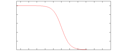
Figure 1: Fermi distribution function at $a>0$.

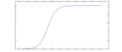
Figure 2: Fermi distribution function at $a<0$.

According to formulas (26) and (27), we can calculate thermodynamical functions of a Fermi gas at low temperature. At $a>0$ the chemical potential is positive $\mu>0$, and the distribution function (22) is plotted in Fig. 1. At $a<0$ the chemical potential is negative $\mu<0$, and the distribution function (22) is given in Fig. 2. So, the distribution function of a Fermi gas can be presented in the universal form

$$f_{p}\left(x,\lambda\right)=\frac{1}{\exp\left[\mathrm{sign}\left(a\right)\left(x-\lambda\right)\right]+1}$$ (28)

where

$$\lambda=\frac{\left|\mu\right|}{T}$$ (29)

Then, taking into account (24) and (25) we can rewrite (26) and (27) in the form

$$n=\frac{\Sigma_{q}}{\left|w\right|}\frac{T^{1/w}}{\left|a\right|^{1/w}}\int\limits_{0}^{\infty}\frac{x^{1/w-1}dx}{\exp\left[\mathrm{sign}\left(a\right)\left(x-\lambda\right)\right]+1}$$ (30)

$$E=\mathrm{sign}\left(a\right)\frac{\Sigma_{q}}{\left|w\right|}\frac{T^{1/w+1}}{\left|a\right|^{1/w}}\int\limits_{0}^{\infty}\frac{x^{1/w+1}dx}{\exp\left[\mathrm{sign}\left(a\right)\left(x-\lambda\right)\right]+1}$$ (31)

The EOS $P=wE$ (1) imposes no restriction concerning the signs of $a$ and $w$ in the energy spectrum (15). The regular matter is characterized by

$$a>0\qquad w>0\qquad\Leftrightarrow\qquad E>0\qquad P>0$$ (32)

while negative $a<0$ and positive $w>0$ corresponds to the material with negative pressure and negative energy density:

$$a<0\qquad w>0\qquad\Leftrightarrow\qquad E<0\qquad P<0$$ (33)

Our main interest is focused on the exotic matter that has negative $w<0$ and whose energy spectrum (15) admits two alternatives

$$a>0\qquad w<0\qquad\Leftrightarrow\qquad E>0\qquad P<0$$ (34)

and

$$a<0\qquad w<0\qquad\Leftrightarrow\qquad E<0\qquad P>0$$ (35)

3 Exotic fermion matter at zero temperature

Consider an ideal Fermi gas whose EOS is $P=wE$. This gas is composed of quasi-particles with the energy spectrum (15). The distribution function of a Fermi gas (28) at low temperature (large $\lambda\gg 1$) reveals the following asymptotic behavior

$$f_{p}\left(0,\lambda\right)=\frac{1}{\exp\left[-\mathrm{sign}\left(a\right)\lambda\right]+1}\cong\Theta\left(a\right)\qquad\underset{x\rightarrow\infty}{\lim}f_{p}\left(x,\lambda\right)=\Theta\left(-a\right)$$ (36)

In other words

$$f_{p}\left(0,\lambda\right)=1\qquad\underset{x\rightarrow\infty}{\lim}f_{p}\left(x,\lambda\right)=0\qquad a>0$$ (37)

and

$$f_{p}\left(0,\lambda\right)=0\qquad\underset{x\rightarrow\infty}{\lim}f_{p}\left(x,\lambda\right)=1\qquad a<0$$ (38)

At very low temperature

$$\lambda\rightarrow\frac{\left|\varepsilon_{F}\right|}{T}$$ (39)

where

$$\varepsilon_{F}=ap_{F}^{wq}$$ (40)

is the Fermi energy and $p_{F}$ is the Fermi momentum, and the distribution function it approaches to the Heaviside step

$$f_{p}\rightarrow\Theta\left[\mathrm{sign}\left(a\right)\left(\left|\varepsilon_{F}\right|/T-x\right)\right]$$ (41)

At zero temperature distribution function is taken in the form

$$f_{p}=\Theta\left(\varepsilon_{F}-\varepsilon_{p}\right)=\Theta\left[\mathrm{sign}\left(a\right)\left(\left|\varepsilon_{F}\right|-\left|\varepsilon\right|\right)\right]$$ (42)

where the energy spectrum is determined by formula (15).

For regular matter (32) the distribution function (42) is equivalent to

$$f_{p}=\Theta\left(p_{F}-p\right)$$ (43)

and limits of integration $p\in\left(0,p_{F}\right)$ correspond to $\varepsilon\in\left(0,\varepsilon_{F}\right)$. At zero temperature $T\rightarrow 0$ formulas (30) and (31) yield

$$n=\frac{\Sigma_{q}}{wa^{1/w}}\underset{T\rightarrow 0}{\lim}\left(T^{1/w}\int\limits_{0}^{\infty}x^{1/w-1}dx\right)=\frac{\Sigma_{q}}{wa^{1/w}}\int\limits_{0}^{\varepsilon_{F}}\varepsilon^{1/w-1}d\varepsilon=\Sigma_{q}\left(\frac{\varepsilon_{F}}{a}\right)^{1/w}=\Sigma_{q}\,p_{F}^{q}$$ (44)

$$E=\frac{\Sigma_{q}}{wa^{1/w}}\left(\underset{T\rightarrow 0}{\lim}T^{1/w+1}\int\limits_{0}^{\infty}x^{1/w}dx\right)=\frac{\Sigma_{q}}{wa^{1/w}}\int\limits_{0}^{\varepsilon_{F}}\varepsilon^{1/w}d\varepsilon=\Sigma_{q}\frac{\varepsilon_{F}^{1/w+1}}{a^{1/w}}=\frac{a\Sigma_{q}}{w+1}p_{F}^{\left(w+1\right)q}$$ (45)

Hence, formulas (44) and (45) imply

$$E=\frac{a}{\left(w+1\right)\Sigma_{q}^{w}}n^{w+1}$$ (46)

Particularly, for the ’absolute stiff’ matter with $w=1$ we have always [6]

$$P=E=\frac{a}{2\Sigma_{q}}n^{2}$$ (47)

For exotic matter (15) with $a>0$ and $w<0$ the distribution function (42) is equivalent to

$$f_{p}=\Theta\left(p-p_{F}\right)$$ (48)

that determines limits of integration $p\in\left(p_{F},\infty\right)$ corresponding to $\varepsilon\in\left(\varepsilon_{F},0\right)$. At zero temperature formulas (30) and (31) yield

$$n=-\frac{\Sigma_{q}}{wa^{1/w}}\underset{T\rightarrow 0}{\lim}\left(T^{1/w}\int\limits_{0}^{\infty}x^{1/w-1}dx\right)=\frac{\Sigma_{q}}{wa^{1/w}}\int\limits_{\varepsilon_{F}}^{0}\varepsilon^{1/w-1}d\varepsilon=q\Sigma_{q}\int\limits_{p_{F}}^{\infty}p^{q-1}dp$$ (49)

$$E=-\frac{\Sigma_{q}}{wa^{1/w}}\left(\underset{T\rightarrow 0}{\lim}T^{1/w+1}\int\limits_{0}^{\infty}x^{1/w}dx\right)=\frac{\Sigma_{q}}{wa^{1/w}}\int\limits_{\varepsilon_{F}}^{0}\varepsilon^{1/w}d\varepsilon=aq\Sigma_{q}\int\limits_{p_{F}}^{\infty}p^{wq}p^{q-1}dp$$ (50)

Integral (49) is divergent at $w<0$, integral (50) is divergent at $0\geq w\geq-1$. At $w<-1$ integral (50) is finite and evaluated as

$$E=-\frac{\Sigma_{q}}{wa^{1/w}}\int\limits_{0}^{\varepsilon_{F}}\varepsilon^{1/w}d\varepsilon=-\frac{\Sigma_{q}}{\left(w+1\right)a^{1/w}}\varepsilon_{F}^{1/w+1}=-\frac{a\Sigma_{q}}{w+1}p_{F}^{\left(w+1\right)q}$$ (51)

However, the particle number density (49) remains undefined. If we introduce an upper cutoff momentum $p_{0}\gg p_{F}$, integral (51) is estimated as

$$n\simeq\Sigma_{q}p_{0}^{q}\gg\Sigma_{q}p_{F}^{q}$$ (52)

but integral (51) remains unchanged

$$E=\frac{a\Sigma_{q}}{w+1}\left[p_{0}^{\left(w+1\right)q}-p_{F}^{\left(w+1\right)q}\right]\simeq-\frac{a\Sigma_{q}}{w+1}p_{F}^{\left(w+1\right)q}$$ (53)

The pressure $P=wE$ is negative, while $P+E<0$ at $w<-1$.

For exotic matter with negative $a<0$ (35) the energy $\varepsilon_{p}$ (15) and the Fermi level $\varepsilon_{F}$ (43) are negative, and distribution function (42) and (LABEL:fx1) implies

$$f_{p}=\Theta\left(\left|\varepsilon_{p}\right|-\left|\varepsilon_{F}\right|\right)$$ (54)

At negative $w<0$ this distribution function is equivalent to (43) but limits of integration $p\in\left(0,p_{F}\right)$ correspond to $\varepsilon_{p}\in\left(-\infty,\varepsilon_{F}\right)$. At zero temperature formulas (30) and (31) yield

$$n=-\frac{\Sigma_{q}}{w\left|a\right|^{1/w}}\left(\underset{T\rightarrow 0}{\lim}T^{1/w}\int\limits_{0}^{\infty}x^{1/w-1}dx\right)=\frac{\Sigma_{q}}{w\left|a\right|^{1/w}}\int\limits_{\infty}^{\left|\varepsilon_{F}\right|}\xi^{1/w-1}d\xi=\Sigma_{q}\left(\frac{\varepsilon_{F}}{a}\right)^{1/w}=\Sigma_{q}\,p_{F}^{q}$$ (55)

$$E=\frac{\Sigma_{q}}{w\left|a\right|^{1/w}}\left(\underset{T\rightarrow 0}{\lim}T^{1/w+1}\int\limits_{0}^{\infty}x^{1/w}dx\right)=-\frac{\Sigma_{q}}{w\left|a\right|^{1/w}}\int\limits_{\infty}^{\left|\varepsilon_{F}\right|}\xi^{1/w}d\xi=-\left|a\right|q\Sigma_{q}\int\limits_{0}^{p_{F}}p^{wq}p^{q-1}dp$$ (56)

Integral (56) is divergent at $w\leq-1$. However, at $0>w>-1$ formulas (55) and (56) are fully integrated, resulting in

$$E=-\frac{\left|a\right|}{\left(w+1\right)\Sigma_{q}^{w}}n^{w+1}<0$$ (57)

that is similar to (46). This exotic matter has negative energy density and positive pressure, meanwhile $P+E<0$.

For exotic matter with negative $a<0$ and positive $w>0$ (33) the distribution function (54) is equivalent to (43). Hence, limits of integration $p\in\left(p_{F},\infty\right)$ will correspond to $\varepsilon_{p}\in\left(-\varepsilon_{F},-\infty\right)$. The particle number density and the energy density are determined by formulas

$$n=\frac{\Sigma_{q}}{w\left|a\right|^{1/w}}\left(\underset{T\rightarrow 0}{\lim}T^{1/w}\int\limits_{0}^{\infty}x^{1/w-1}dx\right)=\frac{\Sigma_{q}}{w\left|a\right|^{1/w}}\int\limits_{\left|\varepsilon_{F}\right|}^{\infty}\xi^{1/w-1}d\xi=q\Sigma_{q}\int\limits_{p_{F}}^{\infty}p^{q-1}dp$$ (58)

$$E=-\frac{\Sigma_{q}}{w\left|a\right|^{1/w}}\left(\underset{T\rightarrow 0}{\lim}T^{1/w+1}\int\limits_{0}^{\infty}x^{1/w}dx\right)=-\frac{\Sigma_{q}}{w\left|a\right|^{1/w}}\int\limits_{\left|\varepsilon_{F}\right|}^{\infty}\xi^{1/w}d\xi=-\left|a\right|q\Sigma_{q}\int\limits_{p_{F}}^{\infty}p^{wq}p^{q-1}dp$$ (59)

Both integrals are divergent, and an upper cutoff momentum is necessary for their estimation.

4 Exotic matter with $E>0$ and $P<0$ at $0>w\geq-1$

Consider formulas (49) and (50) when $0>w\geq-1$. This matter has positive energy density and negative pressure, however, their sum will be non-negative $P+E\geq 0$. Both integrals (49) and (50) are divergent. However, if we introduce the cutoff value of energy

$$\varepsilon_{0}=ap_{0}^{wq}\ll\varepsilon_{F}$$ (60)

corresponding to the cutoff momentum $p_{0}\gg p_{F}$, and change the limits of integration

$$\int\limits_{\varepsilon_{F}}^{0}...d\varepsilon=\underset{\varepsilon_{0}\rightarrow 0}{\lim}\int\limits_{\varepsilon_{F}}^{\varepsilon_{0}}...d\varepsilon$$ (61)

$$\int\limits_{p_{F}}^{\infty}...dp=\underset{p_{0}\rightarrow\infty}{\lim}\int\limits_{p_{F}}^{p_{0}}...dp$$ (62)

then, we obtain finite results that will help us to analyze the behavior of exotic matter. The divergent terms, substracted from integrals (49) and (50), do not depend on temperature and, hence, play no role in the entropy and heat capacity of exotic matter.

So, the particle number density and the energy density are estimated so

$$n=\frac{\Sigma_{q}}{wa^{1/w}}\int\limits_{\varepsilon_{F}}^{\varepsilon_{0}}\varepsilon^{1/w-1}d\varepsilon=\Sigma_{q}\frac{\varepsilon_{0}^{1/w}-\varepsilon_{F}^{1/w}}{\left|a\right|^{1/w}}=\Sigma_{q}\left(p_{0}^{q}-p_{F}^{q}\right)=n_{0}-n_{F}$$ (63)

where

$$n_{F}=\int\limits_{0}^{p_{0}}d^{q}p=\Sigma_{q}p_{F}^{q}$$ (64)

and

$$n_{0}=\int\limits_{0}^{p_{F}}d^{q}p=\Sigma_{q}p_{0}^{q}$$ (65)

The energy density (50) at $0>w>-1$ is estimated by formula

$$E=\frac{\Sigma_{q}}{wa^{1/w}}\int\limits_{\varepsilon_{F}}^{\varepsilon_{0}}\varepsilon^{1/w}d\varepsilon=\frac{\Sigma_{q}}{a^{1/w}}\frac{\varepsilon_{0}^{1/w+1}-\varepsilon_{F}^{1/w+1}}{\left(w+1\right)}=\frac{a\Sigma_{q}}{w+1}\left[p_{0}^{\left(w+1\right)q}-p_{F}^{\left(w+1\right)q}\right]$$ (66)

that is

$$E=\frac{a}{\left(w+1\right)\Sigma_{q}^{w}}\left[n_{0}^{w+1}-\left(n_{0}-n\right)^{w+1}\right]$$ (67)

Since $p_{0}\gg p_{F}$, the particle number density $n=n_{0}-n_{F}$ (66) is approximated by constant value $n\simeq n_{0}$ (52), and the energy density (66) also approximated by a constant value

$$E\simeq\frac{a}{\left(w+1\right)\Sigma_{q}^{w}}n_{0}^{w+1}=B=\mathrm{const}$$ (68)

so that the relevant EOS looks like

$$P\simeq-\left|w\right|B$$ (69)

$$E\simeq B$$ (70)

According to (50), the exotic matter with $w=-1$ will have the energy density

$$E=a\Sigma_{q}\mathrm{\ln}\frac{\varepsilon_{F}}{\varepsilon_{0}}=aq\Sigma_{q}\mathrm{\ln}\frac{p_{0}}{p_{F}}=a\Sigma_{q}\ln\left(\frac{n_{0}}{n_{F}}\right)$$ (71)

slightly dependent on $p_{F}$. Formula (71) bears resemblance with a logarithmic law in the Hagedorn EOS [9] and a logarithmic law in the transition between $w>-1$ and $w<-1$ in the dark energy [5]. Particularly, taking the energy spectrum (17) in a 3-dimensional space, we obtain the EOS

$$E=\frac{\gamma M^{4}}{6\pi^{2}}\ln\left(\frac{p_{0}}{p_{F}}\right)$$ (72)

5 Exotic matter with $E<0$ and $P>0$ at $w\leq-1$

Consider formulas (55) and (56) at $w\leq-1$. This matter has negative energy density and positive pressure (because $a<0$), however, their sum will be non-negative $P+E\geq 0$. Integral (56) is divergent, and again it is necessary to introduce the cutoff value of energy $\varepsilon_{0}=ap_{0}^{wq}$ and momentum $p_{0}\ll p_{F}$ in order to remove divergency

$$\int\limits_{\infty}^{\left|\varepsilon_{F}\right|/T}...dx=\underset{\varepsilon_{0}\rightarrow-\infty}{\lim}\int\limits_{\left|\varepsilon_{0}\right|/T}^{\left|\varepsilon_{F}\right|/T}...dx$$ (73)

and

$$\int\limits_{0}^{p_{F}}...dp=\underset{p_{0}\rightarrow 0}{\lim}\int\limits_{p_{0}}^{p_{F}}...dp$$ (74)

Then, at $w<-1$ the energy density (56) is determined so

$$E=-\frac{\Sigma_{q}}{w+1}\frac{\left|\varepsilon_{F}\right|^{1/w+1}-\left|\varepsilon_{0}\right|^{1/w+1}}{\left|a\right|^{1/w}}=-\frac{\left|a\right|\Sigma_{q}}{w+1}\left[p_{F}^{\left(w+1\right)q}-p_{0}^{\left(w+1\right)q}\right]$$ (75)

that is

$$E=-\frac{\left|a\right|}{\left(w+1\right)\Sigma_{q}^{w}}\left[n_{F}^{w+1}-n_{0}^{w+1}\right]<0$$ (76)

where $n_{F}$ and $n_{0}$ are defined in (64) and (65). Since $p_{0}\ll p_{F}$, the particle number density

$$n=q\Sigma_{q}\int\limits_{p_{0}}^{p_{F}}p^{q-1}dp=\Sigma_{q}\left(p_{F}^{q}-p_{0}^{q}\right)=n_{F}-n_{0}$$ (77)

can be taken in the form $n\simeq n_{F}$ (55), and the energy density (81) is estimated so

$$E\simeq\frac{\left|a\right|\Sigma_{q}}{w+1}p_{0}^{\left(w+1\right)q}=\mathrm{const}=-B$$ (78)

that results in the following EOS:

$$E\simeq-B<0\qquad P=\left|w\right|B>0$$ (79)

At $w=-1$ the energy density (56) is determined so

$$E=-\left|a\right|\Sigma_{q}\ln\frac{\varepsilon_{0}}{\varepsilon_{F}}=-\left|a\right|q\Sigma_{q}\ln\frac{p_{F}}{p_{0}}$$ (80)

that is

$$E=-\left|a\right|\Sigma_{q}\ln\frac{n_{F}}{n_{0}}\simeq-\left|a\right|\Sigma_{q}\ln\frac{n}{n_{0}}$$ (81)

because $n\simeq n_{F}\gg n_{0}$. This formula also bears resemblance with logarithmic laws in the Hagedorn EOS [9] and transition between $w>-1$ and $w<-1$ in the dark energy [dark].

6 Low temperature expansion

Formulas (30)-(LABEL:eew) can be presented in the universal form

$$n=\frac{\Sigma_{q}}{\left|w\right|}\frac{T^{1/w}}{\left|a\right|^{1/w}}J\left(\lambda\right)$$ (82)

and

$$E=\mathrm{sign}\left(a\right)\frac{\Sigma_{q}}{\left|w\right|}\frac{T^{1/w+1}}{\left|a\right|^{1/w}}J\left(\lambda\right)$$ (83)

where integral

$$J\left(\lambda\right)=\int\limits_{0}^{\infty}g\left(x\right)f_{p}\left(x,\lambda\right)dx$$ (84)

includes the distribution function $f_{p}$ (28) and function

$$g\left(x\right)=x^{1/w-1}$$ (85)

or

$$g\left(x\right)=x^{1/w}$$ (86)

corresponding to the particle number density and energy density, respectively.

Integrating by parts, we have

$$J\left(\lambda\right)=\left.G\left(x\right)f_{p}\left(x,\lambda\right)\right|_{0}^{\infty}-\int\limits_{0}^{\infty}G\left(x\right)f_{p}^{\prime}\left(x,\lambda\right)dx$$ (87)

where

$$f_{p}^{\prime}\left(x,\lambda\right)=\frac{\partial f_{p}\left(x,\lambda\right)}{\partial x}=-\frac{\mathrm{sign}\left(a\right)\exp\left[\mathrm{sign}\left(a\right)\left(x-\lambda\right)\right]}{\left\{\exp\left[\mathrm{sign}\left(a\right)\left(x-\lambda\right)\right]+1\right\}^{2}}=-\frac{\mathrm{sign}\left(a\right)\exp\left(x-\lambda\right)}{\left(\exp\left(x-\lambda\right)+1\right)^{2}}$$ (88)

and

$$G\left(x\right)=\int g\left(x\right)dx$$ (89)

Expression

$$J_{0}=\left.G\left(x\right)f_{p}\left(x,\lambda\right)\right|_{0}^{\infty}=\underset{x\rightarrow\infty}{\lim}\left[G\left(x\right)f_{p}\left(x,\lambda\right)\right]-\underset{x\rightarrow 0}{\lim}\left[G\left(x\right)f_{p}\left(x,\lambda\right)\right]$$ (90)

in the light of (37) and (38), is simplified so

$$J_{0}=-\underset{x\rightarrow 0}{\lim}G\left(x\right)\qquad a>0$$ (91)

$$J_{0}=\underset{x\rightarrow\infty}{\lim}G\left(x\right)\qquad a<0$$ (92)

If quantity $J_{0}$ is divergent, then, we introduce some finite cutoff value

$$x_{0}\ll\lambda\qquad a>0$$ (93)

or

$$x_{0}\gg\lambda\qquad a<0$$ (94)

So, we can present $J_{0}$ (91)-(92) in a universal form

$$J_{0}=-\mathrm{sign}\left(a\right)G\left(x_{0}\right)$$ (95)

Therefore, integral (87) is immediately written in the form

$$J\left(\lambda\right)=-\mathrm{sign}\left(a\right)G\left(x_{0}\right)-\int\limits_{0}^{\infty}G\left(x\right)f_{p}^{\prime}\left(x,\lambda\right)dx$$ (96)

Let us expand function $G\left(x\right)$ in the Taylor series [10]

$$G\left(x\right)=G\left(\lambda\right)+\sum\limits_{k=1}^{k=\infty}\frac{g^{\left(k-1\right)}\left(\lambda\right)}{k!}\left(x-\lambda\right)^{k}$$ (97)

where

$$g^{\left(k\right)}\left(x\right)=\frac{\partial^{k}g\left(x\right)}{\partial x^{k}}$$ (98)

Substituting (97) in (96) we have

$$J\left(\lambda\right)=-\mathrm{sign}\left(a\right)G\left(x_{0}\right)-G\left(\lambda\right)\int\limits_{0}^{\infty}f_{p}^{\prime}\left(x,\lambda\right)dx-\sum\limits_{k=1}^{k=\infty}\frac{g^{\left(k-1\right)}\left(\lambda\right)}{k!}\int\limits_{0}^{\infty}\left(x-\lambda\right)^{k}f_{p}^{\prime}\left(x,\lambda\right)dx$$ (99)

In the light of (28)-(38), the first term in (99) is simplified so

$$-G\left(\lambda\right)\int\limits_{0}^{\infty}f_{p}^{\prime}\left(x,\lambda\right)dx=-\left.G\left(\lambda\right)f_{p}\left(x,\lambda\right)\right|_{0}^{\infty}=\mathrm{sign}\left(a\right)G\left(\lambda\right)$$ (100)

Hence

$$J\left(\lambda\right)=-\mathrm{sign}\left(a\right)G\left(x_{0}\right)+\mathrm{sign}\left(a\right)G\left(\lambda\right)-\sum\limits_{k=1}^{k=\infty}\frac{g^{\left(k-1\right)}\left(\lambda\right)}{k!}\int\limits_{0}^{\infty}\left(x-\lambda\right)^{k}f_{p}^{\prime}\left(x,\lambda\right)dx$$ (101)

where $f_{p}^{\prime}\left(x,\lambda\right)$ is determined by (88). At low temperature ($\lambda=\mu/T\gg 1$) integral (101) is approximated by formula

$$J\left(\lambda\right)\cong\mathrm{sign}\left(a\right)\left[G\left(\lambda\right)-G\left(x_{0}\right)+\sum\limits_{k=1}^{k=\infty}g^{\left(k\right)}\left(\lambda\right)C_{k}\right]$$ (102)

with coefficients

$$C_{k}=\frac{1}{k!}\int\limits_{0}^{\infty}\left(x-\lambda\right)^{2k}\frac{\exp\left[\mathrm{sign}\left(a\right)\left(x-\lambda\right)\right]}{\left\{\exp\left[\mathrm{sign}\left(a\right)\left(x-\lambda\right)\right]+1\right\}^{2}}dx=$$

$$\quad=\int\limits_{-\lambda}^{\infty}x^{2k}\frac{\exp\left(x\right)}{\left(\exp\left(x\right)+1\right)^{2}}dx\cong\int\limits_{-\infty}^{\infty}x^{k}\frac{\exp\left(x\right)}{\left(\exp\left(x\right)+1\right)^{2}}dx$$ (103)

Note that all odd coefficients (103) tend to zero

$$C_{2k+1}\rightarrow 0$$ (104)

Integral (102) can be written in explicit form

$$J\left(\lambda\right)=\mathrm{sign}\left(a\right)\left[G\left(\lambda\right)-G\left(x_{0}\right)+g^{\prime}\left(\lambda\right)\frac{\pi^{2}}{6}+g^{\prime\prime\prime}\left(\lambda\right)\frac{7\pi^{4}}{360}+...\right]$$ (105)

that is

$$J\left(\lambda\right)=G\left(\lambda\right)-\underset{x_{0}\rightarrow 0}{\lim}G\left(x_{0}\right)+g^{\prime}\left(\lambda\right)\frac{\pi^{2}}{6}+g^{\prime\prime\prime}\left(\lambda\right)\frac{7\pi^{4}}{360}+...\qquad a>0$$ (106)

and

$$J\left(\lambda\right)=\underset{x_{0}\rightarrow\infty}{\lim}G\left(x_{0}\right)-G\left(\lambda\right)-g^{\prime}\left(\lambda\right)\frac{\pi^{2}}{6}-g^{\prime\prime\prime}\left(\lambda\right)\frac{7\pi^{4}}{360}+...\qquad a<0$$ (107)

For arbitrary function $g\left(x\right)$ formula (105) determines a low temperature expansion of the relevant thermodynamical quantity.

7 Fermi level at low temperature

According to (86) and (89), we have

$$G\left(x\right)=wx^{1/w}$$ (108)

Substituting function (108) in integrals (105), we obtain

$$J\left(\lambda\right)=\mathrm{sign}\left(a\right)\left(w\lambda^{1/w}-wx_{0}^{1/w}+\frac{1-w}{w}\frac{\pi^{2}}{6}\lambda^{1/w-2}\right)$$ (109)

where the cutoff value $x_{0}$ is taken according to (93) and (94).

Substituting (109) in (82) we get the particle number density

$$n=\mathrm{sign}\left(a\right)\mathrm{sign}\left(w\right)\left(n_{F}-n_{0}\right)$$ (110)

where

$$n_{F}=\Sigma_{q}\frac{\left|\mu\right|^{1/w}}{\left|a\right|^{1/w}}\left(1+\frac{1-w}{w^{2}}\frac{\pi^{2}}{6}\frac{T^{2}}{\mu^{2}}\right)$$ (111)

and

$$n_{0}=\Sigma_{q}\frac{\left|\mu_{0}\right|^{1/w}}{\left|a\right|^{1/w}}=\Sigma_{q}p_{0}^{q}=\mathrm{const}$$ (112)

At zero temperature $\mu\rightarrow\varepsilon_{F}$, and formula (111) is reduced to

$$n_{F}=\Sigma_{q}\frac{\left|\varepsilon_{F}\right|^{1/w}}{a^{1/w}}=\Sigma_{q}p_{F}^{q}$$ (113)

that coincides with (64). Hence, the Fermi energy level at low temperature is approximated by formula

$$\left|\mu\right|\cong\left|\varepsilon_{F}\right|\left(1-\frac{1-w}{w}\frac{\pi^{2}}{6}\frac{T^{2}}{\varepsilon_{F}^{2}}\right)$$ (114)

Note that it does not depend on the sign of $a$, neither divergency of play (109) is reflected here.

For nonrelativistic EOS with $w=2/3$ we get a well known expression [10]

$$\mu\cong\varepsilon_{F}\left(1-\frac{\pi^{2}}{12}\frac{T^{2}}{\varepsilon_{F}^{2}}\right)$$ (115)

At $w<0$ the absolute value of Fermi level $\left|\mu\right|$ always exceeds the same at zero temperature $\left|\varepsilon_{F}\right|$, particularly, at $w=-1$ the low-temperature approximation of the Fermi level is the following

$$\left|\mu\right|\cong\left|\varepsilon_{F}\right|\left(1+\frac{\pi^{2}}{3}\frac{T^{2}}{\varepsilon_{F}^{2}}\right)$$ (116)

8 Energy density at low temperature

According to (86) and (89), we have

$$G\left(x\right)=\frac{w}{w+1}x^{1/w+1}\qquad w\neq-1$$ (117)

and

$$G\left(x\right)=\ln x\qquad w=-1$$ (118)

Substituting (117)-(118) in (105), we obtain

$$\mathrm{sign}\left(a\right)J\left(\lambda\right)=\frac{w}{w+1}\lambda^{1/w+1}-\frac{w}{w+1}x_{0}^{1/w+1}+\frac{\lambda^{1/w-1}}{w}\frac{\pi^{2}}{6}+\frac{\left(1-w\right)\left(1-2w\right)}{w^{3}}\frac{7\pi^{4}}{360}\lambda^{1/w-3}$$ (119)

when $w\neq-1$, while

$$\mathrm{sign}\left(a\right)J\left(\lambda\right)=\ln\frac{\lambda}{x_{0}}-\frac{\pi^{2}}{6}\frac{1}{\lambda^{2}}-\frac{7\pi^{4}}{60}\frac{1}{\lambda^{4}}$$ (120)

when $w=-1$. The cutoff value $x_{0}=\varepsilon_{0}/T$ is taken from conditions (93) and (94) in accordance to the sign of $a$.

Substituting (119) in (83) we find the energy density

$$E=\frac{\mathrm{sign}\left(w\right)}{w+1}\frac{\Sigma_{q}}{\left|a\right|^{1/w}}\left\{\left|\mu\right|^{1/w+1}\left[1+\frac{w+1}{w^{2}}\frac{\pi^{2}}{6}\frac{T^{2}}{\mu^{2}}+\frac{\left(1-w^{2}\right)\left(1-2w\right)}{w^{4}}\frac{7\pi^{4}}{360}\frac{T^{4}}{\mu^{4}}\right]-\left|\varepsilon_{0}\right|^{1/w+1}\right\}$$ (121)

when $w\neq-1$. Substituting (120) in (83) we find the energy density

$$E=\frac{\Sigma_{q}}{\left|a\right|^{1/w}}\left[\ln\frac{\left|\mu\right|}{\left|\varepsilon_{0}\right|}-\frac{\pi^{2}}{6}\frac{T^{2}}{\mu^{2}}-\frac{7\pi^{4}}{60}\frac{T^{4}}{\mu^{4}}\right]$$ (122)

when $w=-1$. We can check formula (121) for regular ultrarelativistic matter with EOS $P=E/3$ and in 3-dimensional space [11]

$$P=\frac{E}{3}=\frac{\gamma}{24\pi^{2}}\left(\mu^{4}+2\pi^{2}T^{2}\mu^{2}+\frac{7\pi^{4}}{15}T^{4}\right)$$ (123)

Substituting (114) in (121), we obtain a low-temperature expansion of the energy density at $w\neq-1$:

$$E=\frac{\mathrm{sign}\left(w\right)}{w+1}\frac{\Sigma_{q}}{\left|a\right|^{1/w}}\left[\left|\varepsilon_{F}\right|^{1/w+1}\left(1+\frac{w+1}{w}\frac{\pi^{2}}{6}\frac{T^{2}}{\left|\varepsilon_{F}\right|^{2}}\right)-\left|\varepsilon_{0}\right|^{1/w+1}\right]$$ (124)

Formula (124) can rewritten so

$$E=E_{0}+\frac{\pi^{2}}{6}\Sigma_{q}\frac{\left|\varepsilon_{F}\right|^{1/w+1}}{\left|w\right|\left|a\right|^{1/w}}\frac{T^{2}}{\left|\varepsilon_{F}\right|^{2}}$$ (125)

where

$$E_{0}=\frac{\mathrm{sign}\left(w\right)}{w+1}\frac{\Sigma_{q}}{\left|a\right|^{1/w}}\left(\left|\varepsilon_{F}\right|^{1/w+1}-\left|\varepsilon_{0}\right|^{1/w+1}\right)=\frac{\mathrm{sign}\left(w\right)}{\left(w+1\right)}\frac{\left|a\right|}{\Sigma_{q}^{w}}\left(n_{F}^{w+1}-n_{0}^{w+1}\right)$$ (126)

is the energy density at zero temperature. Expression (126) embraces formulas (45), (50), (56) and (80) when $w\neq-1$.

Substituting (114) in (122), we obtain a low-temperature expansion of the energy density at $w=-1$:

$$E=E_{0}+\frac{\pi^{2}}{6}\Sigma_{q}\left|a\right|\frac{T^{2}}{\left|\varepsilon_{F}\right|^{2}}$$ (127)

where

$$E_{0}=\Sigma_{q}\left|a\right|\ln\frac{\left|\varepsilon_{F}\right|}{\left|\varepsilon_{0}\right|}=\Sigma_{q}\left|a\right|\ln\frac{n_{0}}{n_{F}}$$ (128)

is the energy density at zero temperature, that coincides with (71) and (80).

9 Entropy and heat capacity at low temperature

Expressions (125) and (127) allow to obtain the entropy density $S$ and the heat capacity $C_{V}$ according to standard formulas [12]

$$S=-\frac{\partial\left(T\ln Z\right)}{\partial T}=\frac{\partial P}{\partial T}\qquad C_{V}=T\frac{\partial S}{\partial T}$$ (129)

where the pressure is $P=wE$ (1). Substituting (125) and (127) in (129), we find general formula

$$S=C_{V}=\mathrm{sign}\left(w\right)\frac{\pi^{2}}{3}\Sigma_{q}\frac{T\left|\varepsilon_{F}\right|^{1/w-1}}{\left|a\right|^{1/w}}=\mathrm{sign}\left(w\right)\frac{\pi^{2}}{3}\Sigma_{q}\frac{T}{\left|\varepsilon_{F}\right|}p_{F}^{q}=\mathrm{sign}\left(w\right)\frac{\pi^{2}}{3}\frac{T}{\left|\varepsilon_{F}\right|}n_{F}$$ (130)

which is valid for any $w$. The density $n_{F}$ is defined by (113). Particularly, at $w=1$ the heat capacity is

$$S=C_{V}=\frac{\pi^{2}}{3}\Sigma_{q}\frac{T}{\left|a\right|}$$ (131)

that after parametrization $a=m^{2}$ yields the heat capacity of ’absolute stiff’ matter [6]. The regular nonrelativistic Fermi gas with the energy spectrum $\varepsilon_{p}=\frac{p^{2}}{/}(2m)$ and EOS $P=2/3E$ yields has the heat capacity [10]

$$S=C_{V}=\frac{\pi^{2}}{3}\Sigma_{q}m^{3/2}\sqrt{\left|\varepsilon_{F}\right|}T$$ (132)

The sign of the energy density $E$ is not sufficient, but the sign of $w$ play the main role, and exotic fermion matter with $w<0$ will have negative entropy and negative heat capacity, particularly

$$S=C_{V}=-\frac{\pi^{2}}{3}\Sigma_{q}\frac{\left|a\right|T}{\left|\varepsilon_{F}\right|^{2}}$$ (133)

at $w=-1$.

10 Conclusion

For and arbitrary relation between the pressure and energy density $P=wE$ (1) at constant $w$, the EOS can be modeled by and ideal gas of free quasi-particles with the universal energy spectrum $\varepsilon_{p}=ap^{wq}$ (15). The sign of $w$ and $a$ can be arbitrary, and thermodynamical functions of this gas are determined by formulas (30) and (31). We have analyzed in detail a Fermi gas of such quasi-particles at zero temperature.

For regular matter with positive pressure $P>0$ and positive energy density $E>0$ (correspond to $w>0$ and $a>0$), the particle number density $n$ and energy density $E$ are given by formulas (44), (45), and (LABEL:ee11).

For exotic matter with negative pressure $P<0$ and positive energy density $E>0$ ($w<0$ and $a>0$), the particle number density and energy density are given by formulas (49) and (50). At $w<-1$, when $P+E<0$, the energy density is given by formula (51) which characterizes the regular matter (45) and reveals proportionality

$$E\sim n^{w+1}$$ (134)

At $w\geq-1$ the energy density is divergent, and a cutoff momentum $p_{0}$ is introduced for its estimation. At $w=-1$ the energy density is given by formula (53) and at $0>w>-1$ (when $P+E>0$) the energy density attains constant value (68) which depends on $p_{0}$. However, the law (134) is not working now, but the matter admits description in the frames of the ’bag’ model $P=-E=\mathrm{const}$.

For exotic matter with positive pressure $P>0$ and negative energy density $E<0$ ($w>0$ and $a<0$), the particle number density and energy density are given by formulas (55) and (56). At $0>w>-1$ (when $P+E<0$), the energy density is given by formula (57) which obeys the law (134).

At $w\leq-1$ the energy density is divergent, and a cutoff momentum $p_{0}$ is introduced again for its estimation. At $w=-1$ the energy density is given by formula (81), while at $w<-1$ (when $P+E>0$), the energy density attains constant value (78). Again, proportionality (134) is not valid now.

In order to estimate the thermodynamical functions of Fermi gas at finite temperature, it is necessary to develop formulas (84), (84), (106), (107). The particle number density $n$ at low temperature is determined by expressions (110)-(112). The Fermi level $\mu$ at low temperature is determined by formula (114). Its peculiar property is that it exceeds the Fermi level at zero temperature $\varepsilon_{F}$ when $1>w>0$, meanwhile $\mu<\varepsilon_{F}$ when $w<0$ or when $w>1$. A low-temperature expansion of the energy density is determined by formula (124) at $w\neq-1$, and by formula (127) at $w=-1$. The entropy density and heat capacity at low temperature is given by the single formula (130). It is linear dependent on temperature. However, exotic matter with negative $w<0$ has negative entropy and negative heat capacity, see, for example, formula (133) at $w=-1$.

The theory of ideal Fermi gas of quasi-particles in 3-dimensional space (whose energy spectrum is $\varepsilon_{p}=ap^{3w}$) can be immediately applied to compact stellar objects containing hypothetical material with arbitrary EOS $P=wE$, where $w$ is constant. However, we should not forget that the central pressure must be positive. Only the regular matter ($a>0$ and $w>0$) and exotic matter with positive pressure and negative energy density (when $a<0$ and $w<0$) are suitable for stable stellar models. Calculations are in progress.

For the EOS $P=-E$ the energy density and particle number density at zero temperature have a logarithmic link (128) similar to the Hagedorn EOS. This also deserves more analysis.

The authors are grateful to Erwin Schmidt for discussions.

References

• [1] E. Trojan and G. V. Vlasov, Phys. Rev. D 83, 124013 (2011). arXiv:1103.2276 [hep-ph]
• [2] E. Trojan and G. V. Vlasov, Tachyonic thermal excitations and causality. arXiv:1106.5857 [hep-ph]
• [3] A. Melchiorri, L. Mersini, C. J. Odman, and M. Trodden, Phys. Rev. D 68, 043509 (2003). arXiv:astro-ph/0211522
• [4] S. M. Carroll, M. Hoffman and M. Trodden, Phys. Rev. D 68, 023509 (2003). arXiv:astro-ph/0301273
• [5] H. Ε tefančiΔ‡, Phys. Rev. D 71, 124036 (2005). arXiv:astro-ph/0504518
• [6] E. Trojan and G. V. Vlasov, Thermodynamics of absolute stiff matter. arXiv:1107.1782 [astro-ph.CO]
• [7] M. Dreizler and E. K. U. Gross, Density functional theory (Springer, 1990), p. 10. C. Speicher, R. M. Dreizler and E. Engel, Ann. Phys. (NY) 213, 312 (1992).
• [8] J. I. Kapusta, Finite-temperature field theory (Cambridge Univ. Press, Cambridge, 1989), p. 8.
• [9] C.E. Rhoades and R. Ruffini, Astrophys. J. 163, L83 (1971).
• [10] J. M. Ziman, Principles of the Theory of Solids (Cambridge Univ. Press, Cambridge, 1972), p. 137.
• [11] D. D. Dixon, P. Kaus, J. Wudka, Phys.Rev. D 55, 6344 (1997). arXiv:hep-ph/9703202
• [12] L. D. Landau and E. M. Lifshitz, Statistical physics, Part I , 3rd ed. (Pergamon Press, Oxford, 1980), p. 46.