The effect of winning an Oscar Award on survival: Correcting for healthy performer survivor bias with a rank preserving structural accelerated failure time model

Abstract

We study the causal effect of winning an Oscar Award on an actor or actress’s survival. Does the increase in social rank from a performer winning an Oscar increase the performer’s life expectancy? Previous studies of this issue have suffered from healthy performer survivor bias, that is, candidates who are healthier will be able to act in more films and have more chance to win Oscar Awards. To correct this bias, we adapt Robins’ rank preserving structural accelerated failure time model and $g$-estimation method. We show in simulation studies that this approach corrects the bias contained in previous studies. We estimate that the effect of winning an Oscar Award on survival is 4.2 years, with a $95\%$ confidence interval of $[-0.4,8.4]$ years. There is not strong evidence that winning an Oscar increases life expectancy.

, , and

1 Introduction

Does an increase in a social animal’s social “rank” cause the animal to live longer? This question has been studied extensively in both nonhuman primates and humans. Animals with social ranks that experience more stress have been shown to experience adverse adrenocortical, cardiovascular, reproductive, immunological, and neurobiological consequences [Sapolsky (2005)]. Redelmeier and Singh (2001) studied the impact of social rank on lifetime in an intriguing context: among Hollywood actors and actresses, does winning an Oscar Award (Academy Award) cause the actor’s/actress’s expected lifetime to increase? In Redelmeier and Singh’s most emphasized comparison (the one cited in their abstract), they stated that life expectancy was 3.9 years longer for Oscar Award winners than for other less recognized performers and that this difference corresponded to a $28\%$ mortality rate reduction for winners compared to less recognized performers ($95\%$ CI: $10\%$ to $42\%$). In an interview, Dr. Redelmeier stated, “Once you’ve got that statuette on your mantel place, it’s an uncontested sign of peer approval that nobody can take away from you, so that any subsequent harsh reviews leave you more resilient. It doesn’t quite get under your skin. The normal stresses and strains of everyday life do not drag you down.” [Associated Press Story, February 26 (2005)].

In Redelmeier and Singh’s analysis emphasized in their abstract, they fit a Cox proportional hazards model with whether a performer ever wins an Oscar Award in his or her lifetime treated as a time-independent covariate and survival measured from the performer’s date of birth. Sylvestre, Huszti and Hanley (2006) pointed out that this analysis suffers from immortal time bias—for a winner, the time before winning is “immortal time.” In other words, performers who live longer have more opportunities to win Oscar Awards. To eliminate immortal time bias, Sylvestre et al. fit a Cox proportional hazards model with winning status treated as a time-dependent covariate and survival measured from a performer’s date of first nomination (Redelmeier and Singh also fit one time-dependent covariate model with survival measured from the performer’s date of birth). Sylvestre et al. estimated that winning an Oscar Award had a positive effect on lifetime, but the estimated effect was not significant. Although a valuable step forward, Sylvestre et al.’s analysis still suffers from healthy performer survivor bias: Candidates who are healthier will be able to act in more films and have more chances to win Oscar Awards. We provide a more detailed description of healthy performer survivor bias in Sections 2 and 3.

In this paper we adapt James Robins’ rank preserving structural accelerated failure time model with $g$-estimation [Robins (1992); Robins et al. (1992)] to eliminate healthy performer survivor bias; it also eliminates immortal time bias, which can be seen as one aspect of healthy performer survivor bias. Our analysis is based on the assumption that the winner of each award is selected randomly among the nominees conditional on age at time of nomination, number of previous nominations and number of previous wins. We first show in a simulation study the potential for healthy performer survivor bias to make inferences from Cox models, with or without time-dependent covariates, incorrect, and then show that $g$-estimation provides correct inferences. We then analyze the effect of winning an Oscar on life expectancy using $g$-estimation.

Our study also contributes to the debate that high socio-economic status is associated with good health and long life. Famous examples are the Whitehall studies of British civil servants; see Reid et al. (1974), Marmot, Rose and Hamilton (1978), Marmot, Shipley and Rose (1984), Marmot et al. (1991) and Ferrie et al. (2002). Recently, Rablen and Oswald (2008) studied the causal effect of winning a Nobel Prize on scientists’ longevity. Correcting for potential bias, they estimated that winning the Nobel Prize, compared to merely being nominated, is associated with between 1 and 2 years of extra longevity. Abel and Kruger (2005) studied the longevity of Baseball Hall of Famers compared to the other players. They concluded that median post-induction survival for Hall of Famers was 5 years shorter than for noninducted players, which does not support the role of celebrity on longevity.

The rest of our paper is organized as follows: Section 2 discusses previous methods and their biases and presents a simulation study that documents these biases, Section 3 describes the rank preserving structural failure time model and $g$-estimation, Section 4 analyzes the Oscar Award data and Section 5 provides conclusion and discussion.

2 Existing methods and biases

2.1 Background for Oscar Awards

The Oscar Awards are the most prominent and most watched film awards ceremony in the world. They are presented annually by the Academy of Motion Pictures Arts and Sciences. We will focus on the awards in four categories—Best Lead Actor, Best Lead Actress, Best Supporting Actor, and Best Supporting Actress. The annual awards selection process is complex, but the brief schedule is as follows: In December, the Academy compiles a list of eligible performers for an award. In January, all Academy members nominate five performers in each of the four categories (Best Lead Actor, Best Lead Actress, Best Supporting Actor, Best Supporting Actress). In February, nominations for each performer are tabulated, and the top five are publicly identified as nominees for each category. Then all Academy members vote for one out of five nominees, and the winner is the one who gets the most votes.

2.2 Previous work

Redelmeier and Singh (2001) compiled a list of all nominees for the Oscar Awards from 1929 to 2000 (72 years). They also matched each nominee to a cast member who performed in the same film as the nominee and was the same sex and born in the same era as the nominee. Redelmeier and Singh’s analysis was based on comparing 235 Oscar winners to 527 nonwinning nominees, and 887 performers who were never nominated (controls). In their primary analysis, survival was measured from performers’ dates of birth. In most of Redelmeier and Singh’s analyses, they used the winner status as a fixed-in-time covariate, that is, a performer would be considered a winner throughout the study if he or she won an Oscar Award at least once in his or her lifetime. Kaplan–Meier curves showed that life expectancy was 3.9 years longer for winner than for controls, and 3.5 years longer for winners than for nonwinning nominees. In Cox proportional hazards models with no adjustment for other covariates, winning was estimated to reduce mortality by $28\%$ compared to controls and by $26\%$ compared to nonwinning nominees, with lower $95\%$ confidence limits for both comparisons greater than $0\%$, suggesting that winning an Oscar has a beneficial effect on lifetime. Adjustment for demographic and professional factors yielded similar results, with lower confidence limits for the mortality reduction due to winning remaining above $0\%$. Redelmeier and Singh considered one Cox proportional hazard model that used the winner status as a time-dependent covariate, that is, an Oscar Award winning performer is treated as a winner only after he or she won an Award. This model estimated a mortality rate reduction of $20\%$ for winners vs. controls, with a lower $95\%$ CI limit of $0\%$.

Sylvestre, Huszti and Hanley (2006) pointed out that analyses that treat winner status as a fixed in time covariate credit the winners’ lifetime before winning toward survival subsequent to winning. These “immortal” years will cause bias in the estimate of the causal effect of winning. We will focus on Sylvestre et al.’s method for correcting this bias in comparing winners to nonwinning nominees. Sylvestre et al. used a Cox proportional hazard model that differed in two ways from Redelmeier and Singh’s primary analyses: (1) winning was treated as a time-dependent covariate, an Oscar Award winning performer only becomes a winner after he or she wins an award (as noted above, Redelmeier and Singh also considered this approach in one of their analyses); (2) a performer was only part of the risk set once he or she was first nominated. Using this model, Sylvestre et al. estimated a mortality rate reduction of $18\%$ for winners vs. nonwinning nominees with a $95\%$ CI of $-4\%$ to $35\%$. Thus, this model estimates that winning an Oscar has a beneficial effect on lifetime, but there is not strong evidence for a beneficial effect. Note that Sylvestre et al. used an updated data set compared to Redelmeier and Singh’s; Sylvestre et al. considered a selection interval for Oscar Awards from 1929 to 2001 (73 years) with 238 winners and 528 nonwinning nominees. Sylvestre, Huszti and Hanley (2006) also used the survival analysis method suggested by Efron (2002) and did an analysis with a binomial logistic regression model. Death in each year of a performer’s life was treated as a Bernoulli random variable and regressed on covariates such as winning status, age of nomination, and calendar year of nomination. This model yielded a similar result as Sylvestre et al.’s Cox proportional hazards model analysis. The results from previous studies are listed in Table 1.

Table 1: Winners vs. nominees

			Reduction in
			mortality rate
Type of analysis	Status	Time-zero	(95% CI) (%)
PHb1	Staticb3	Birthday	23 (3 to 39)$-1$
PH	Dynamicb4	Birthday	11 ($-12$ to 30)
PH	Dynamic	Nomination day	18 ($-4$ to 35)0
PYb2	Dynamic	Nomination day	18 ($-4$ to 36)0

[]Notes: These results are based on the updated data set in Sylvestre, Huszti and Hanley (2006). The first row is the Cox model without adjustment for any covariates; the second row is the Cox model with winning status as a time-dependent covariate and with sex and year of birth as time-independent covariates; the third row is the Cox model with the same covariates as the second row, but with nomination day as time-zero; the fourth row is the binomial logistic regression model with sex, age, and calendar year as covariates. The first two rows are from Redelmeier and Singh’s analysis (using Sylvestre et al.’s updated data set), and the last two rows are from Sylvestre et al.’s analysis. [1]b1PH stands for Cox proportional hazard model. [2]b2PY stands for performer years analysis, which is the binomial logistic regression model described above. [3]b3Static status treats the winning status as a fixed-in-time covariate. [4]b4Dynamic status treats the winning status as a time-dependent covariate.

2.3 Healthy performer survivor bias

Previous studies have suffered from healthy performer survivor bias, that is, candidates who are healthier will be able to act in more films and have more chances to win Oscar Awards.

One aspect of healthy performer survivor bias is immortal time bias, that is, candidates will have more chances to win Oscar Awards if they live longer. When a performer is classified as a winner throughout the study, regardless of when the performer wins the award, there are unfair comparisons between winners and nonwinning performers who died before the winner won the award. As an example, consider Henry Fonda and Dan Dailey, who were both first nominated for an Oscar Award at the age of 35 but did not win in their first nominations. Fonda first won an Oscar at age 77 and died four months after, while Dailey never won an Oscar and died at age 64. Fonda lived 13 years beyond the age of Dailey’s death before winning an Oscar. It is not fair to consider the 13 years before Fonda won his Oscar as being affected by winning.

To correct for immortal time bias, Sylvestre et al. used a Cox proportional hazard model with the winning status as a time-dependent covariate. In this model, the survival comparison between a winner and a nonwinning nominee starts appropriately only at the time the winner wins.

Although Sylvestre et al.’s analysis was an important advance in that it corrects for immortal time bias, it still suffers from other aspects of the healthy performer survivor bias. Winning an Oscar Award is an indicator of being healthy. In Sylvestre et al.’s analysis, the risk set at a given age consists of those performers who have been nominated by that age. Among these performers, those who are healthy at the given age have had more opportunities to perform and to win an Oscar. These healthy performers are also more likely to live longer. Since having won an Oscar is associated with survival in a risk set even if winning has no causal effect on survival, there is the potential for bias.

As an example consider Jack Palance and Arthur O’Connell who were first nominated for Oscars but did not win at ages 34 and 48, respectively. Palance won an Oscar at age 73, while O’Connell never won an Oscar. Palance was an active actor when he was in his 70s, acting in ten films in his 70s, and lived to be 87. On the other hand, O’Connell was stricken with Alzheimer’s disease by the time he turned 70 and by the time of his death at age 73, he was appearing solely in toothpaste commercials (www.imdb.com). The fact that Palance lived longer than O’Connell in the risk set that started at age 73 after Palance’s first win is not likely due to the effect of winning but to the healthy performer survivor bias.

One way of attempting to control for healthy performer survivor bias is to condition on (control for) confounders in the Cox model. In particular, nomination history is a confounder because it is a strong risk factor for subsequently winning on Oscar Award (indeed, it is necessary) and for mortality, since sick individuals do not get nominated. Previous studies did not condition on nomination history and thus suffered from confounding bias.

However, even if we condition on nomination history, as well as past age and Oscar wins, and there are no other confounders besides these variables, the time-dependent Cox model can be biased if Oscar winning affects future nominations [Robins (1986, 1992)]. It is substantively plausible that previous Oscar winning affects future nomination (even under the stronger null hypothesis that neither nomination nor winning affects health). The effect could go in either direction. For example, among two subjects with the same nomination history, only one of whom won before, the winner would have a higher probability of being renominated if increased fame coming from previously winning results in an increased chance of nomination per film, all else being equal. On the other hand, the winner would have a lower probability of being renominated if nominators felt those who have not won before are more deserving of a chance to win.

To understand the bias in the Cox analysis when previous Oscar winning affects future nomination, suppose a previous winner has a higher probability of being renominated, all else being equal. Then one would expect that among the nominees in a given year with same past nomination histories, the previous winners would be less healthy than the previous nonwinners, since the nonwinners might have had to be in a large number of movies in the previous year to get nominated for one of them, while for the winner it often would suffice to be in just one. But only a healthy person could be in many movies in one year. Note that this bias persists even if we had data on the number of movies performed in each year and adjusted for this variable as well as nomination.

2.4 Simulation studies

To illustrate the potential of previous studies of survival in Oscar Award winning performers to suffer from healthy performer survivor bias, we conducted a simulation study.

We first assigned a lifetime for each performer and a time at when the performer became sick. Then for each year, we randomly pick nominees from performers who are still alive and healthy, and randomly select one of them as the winner. Hence, winning an award does not have any effect on prolonging performers’ lifetime, because lifetime is predetermined before deciding who wins the awards. If a method shows an effect of winning over repeated simulations from this setting, it is biased.

For each year between 1830 and 1999, we simulated five performers being born. Each performer was randomly selected to have one of the three age patterns shown in Table 2.

Table 2: Performers’ age pattern

	Sick age	Death age
Group 1	60	70
Group 2	70	80
Group 3	80	90

Table 3: Selection weight for age 60–69

	Previous winner	Previous nonwinner
Group 1	0	0
Group 2	8	1
Group 3	9	7

For each year from 1927 to 2004, we have one award and we select 5 nominees from those performers who are still alive and healthy. The details are that we select two nominees from the age group 30–39, and one from 70–79, selecting randomly among healthy performers in those age groups. We also select two nominees from the age group 60–69, but with different selection probabilities for healthy performers in this age group. For age group 60–69, the selection weight for a healthy candidate is in Table 3.

In this sense, for age group 60–69, winning in the past increases the chance to be selected as a nominee, and previous nonwinners tend to be healthier than previous winners (i.e., in Group 3 rather than in Group 2). This corresponds to the fact that previous nonwinners might have had to be in a large number of movies in the previous year to get nominated for one of them, while for the previous winners it often would suffice to be in just one film to get nominated. Consequently, nominated previous winners tend to be less healthy than nominated previous nonwinners, because nominated previous nonwinners tend to be very healthy to be able to act in many films.

Nominees from different age groups have a different probability to be selected as the winner, with older nominees having a better chance. The winning probability also depends on the nomination history and winning history. Let $1_{30}$, $1_{60}$, and $1_{70}$ be the indicators of current nomination age group 30–39, 60–69, and 70–79, respectively. Let $N_{30}$, $N_{60}$, $N_{70}$ be the number of previous nominations in the age group 30–39, 60–69, and 70–79, respectively. Let $W_{30}$, $W_{60}$, $W_{70}$ be the number of previous wins in the age group 30–39, 60–69, and 70–79, respectively. The winning probability for each nominee in a given year is calculated as

$$P(A_{i}=1|\underline{N_{i}},\underline{A_{i}})$$

$$\qquad=\exp\bigl{(}0.5*1_{30}^{i}+1_{60}^{i}+2*1_{70}^{i}$$

$$\qquad\quad\hphantom{\exp\bigl{(}}{}+0.5(N_{30}^{i}+N_{60}^{i}+N_{70}^{i}+W_{30}^{i}+W_{60}^{i}+W_{70}^{i})\bigr{)}$$

$$\qquad\quad{}\Bigl{/}\sum_{j=1}^{5}\exp\bigl{(}0.5*1_{30}^{j}+1_{60}^{j}+2*1_{70}^{j}$$

$$\qquad\quad\hphantom{/\sum_{j=1}^{5}\exp\bigl{(}}{}+0.5(N_{30}^{j}+N_{60}^{j}+N_{70}^{j}+W_{30}^{j}+W_{60}^{j}+W_{70}^{j})\bigr{)}.$$

We choose these coefficients to magnify the healthy performer survivor bias.

In our simulation setting, death ages are determined before winning, thus winning has no causal effect on lifetime. Therefore, for the null hypothesis that there is no treatment effect of winning an Oscar Award on an actor’s survival, the $p$-values should be uniformly distributed between 0 and 1, and the mean of $p$-values should be around 0.5. If the mean of $p$-values from a method is much smaller than 0.5, then the method is biased.

The results from 1000 simulations are shown in Table 4 and histograms of $p$-values can be found in Figure 3 of Section 3.5.

Table 4: Simulation results

Type of analysis	Status	Time-zero	Mean of $\bolds{p}$-value
PH	Static	Birthday	0.03
PH	Dynamic	Birthday	0.12
PH	Dynamic	Nomination day	0.12
PY	Dynamic	Nomination day	0.04

Redelmeier and Singh’s results were based on the first two methods in Table 4, and Sylvestre et al.’s results were based on the last two methods in Table 4. All of these four methods are biased.

In our simulation setting, past winning history affects future nominations, and past nomination history also affects future winning. The previous methods did not account for the nomination history in the time-dependent Cox model. Next we will show that even if one correctly models the effect of nomination history on the hazard of death, the hazard model still provides biased estimates of the causal effect of winning on survival.

To simplify the consideration of nomination history and winning history, we restrict every candidate to be nominated at most twice and win at most twice. Let $D_{70}$ and $D_{80}$ denote death at age 70 and 80, respectively. Let $S_{69}$ and $S_{79}$ denote survival at age 69 and 79, respectively. Let $N(30)$ and $N(60)$ denote the numbers of nominations in the age group 30–39 and 60–69, respectively. Let $A(30)$ and $A(60)$ denote the numbers of wins in the age group 30–39 and 60–69, respectively. Based on 1000 Monte Carlo simulations, we obtained estimated mortality hazard rates and corresponding $95\%$ confidence intervals for this full model in Tables 5 and 6.

=230pt Mortality rates $\bolds{N(30)}$ $\bolds{A(30)}$ $\bolds{N(60)}$ $\bolds{A(60)}$ (95% CI) 2 2 0 0 0.355 (0.299, 0.411) 2 1 0 0 0.349 (0.332, 0.366) 2 0 0 0 0.327 (0.320, 0.334) 1 1 0 0 0.508 (0.494, 0.523) 1 0 0 0 0.407 (0.404, 0.410) 0 0 0 0 0.380 (0.378, 0.381)

Table 5: Mortality rates for death at 70 conditional on survival to 69 with nomination history and winning history when nomination is affected by past winning history

Table 6: Mortality rates for death at 80 conditional on survival to 79 with nomination history and winning history when nomination is affected by past winning history

						Mortality rates
$\bolds{N(30)}$	$\bolds{A(30)}$	$\bolds{N(60)}$	$\bolds{A(60)}$	$\bolds{N(70)}$	$\bolds{A(70)}$	(95% CI)
2	2	0	0	0	0	0.472 (0.401, 0.544)
2	1	0	0	0	0	0.511 (0.489, 0.534)
2	0	0	0	0	0	0.493 (0.484, 0.502)
1	1	0	0	0	0	0.555 (0.533, 0.577)
1	0	0	0	0	0	0.674 (0.669, 0.678)
1	1	1	1	0	0	0.474 (0.437, 0.511)
1	1	1	0	0	0	0.468 (0.444, 0.492)
1	0	1	1	0	0	0.191 (0.177, 0.206)
1	0	1	0	0	0	0.190 (0.184, 0.196)
0	0	1	1	0	0	0.439 (0.418, 0.460)
0	0	1	0	0	0	0.521 (0.514, 0.528)
0	0	2	2	0	0	0.137 (0.119, 0.155)
0	0	2	1	0	0	0.092 (0.087, 0.098)
0	0	2	0	0	0	0.039 (0.036, 0.041)
0	0	0	0	0	0	0.617 (0.615, 0.619)

For a reduced model without winning history, the mortality rates just adjusting the nomination history are shown in Table 7. From the above probabilities, we can see even though winning has no causal effect on survival, winning history affects the hazard of death given nomination history, for example, the hazard of dying at 80 for people with one nomination during their 30s and no further nominations is much higher for people who did not win an award (0.674) than for those who won one award (0.555).

If we consider a discrete time hazard model, the mortality rate can be modeled as follows:

$$h=\frac{1}{1+\exp(-\sum_{i}\alpha_{i}Z_{i})},$$

where $h$ is the mortality rate, and $Z_{i}$ is the indicator function of nomination and winning history in the full model, or the indicator function of nomination history in the reduced model. Then we can estimate the coefficients $\alpha_{i}$ based on the mortality rates calculated above. With this discrete time hazard model, we can calculate the log likelihood of the full model and the reduced model for each simulation round. Because

$$-2\bigl{(}\mathit{loglikelihood}(\mbox{Reduced Model})-\mathit{loglikelihood}(\mbox{Full Model})\bigr{)}\stackrel{{\scriptstyle D}}{{\rightarrow}}\chi_{12}^{2}$$

when the reduced model is true, we can obtain approximate $p$-values for the test of whether winning has an effect on mortality given nomination history. If the mean of $p$-values is significantly different from 0.5, then it shows that even if one has a correct model for the conditional hazard of death given all the measured time-dependent confounding factors, the model still provides a biased estimate of the effect of winning on survival.

=230pt Mortality rates Death age $\bolds{N(30)}$ $\bolds{N(60)}$ $\bolds{N(70)}$ (95% CI) 70 2 0 0.331 (0.324, 0.337) 70 1 0 0.413 (0.410, 0.416) 70 0 0 0.380 (0.378, 0.381) 80 2 0 0 0.495 (0.487, 0.503) 80 1 0 0 0.668 (0.664, 0.672) 80 1 1 0 0.227 (0.222, 0.232) 80 0 1 0 0.513 (0.506, 0.519) 80 0 2 0 0.059 (0.057, 0.062) 80 0 0 0 0.617 (0.616, 0.619)

Table 7: Mortality rates conditional on nomination history when nomination is affected by past winning history

The mean of $p$-values over 1000 simulation round is 0.404, showing that there is bias. The histograms of $p$-values and test statistics are shown in Figure 1.

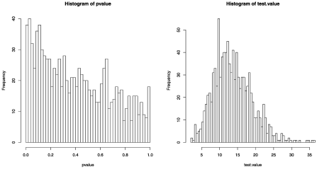
Figure 1: Histograms for $p$-values and test statistics from the likelihood ratio test of whether winning has an effect on mortality given nomination history based on the discrete time hazard model when the nomination is affected by past winning history.

In the above simulation setting, nomination history is both a confounder for winning history’s effect on survival and has been affected by winning history. We now show that if nomination history is only a confounder and has not been affected by winning history, then the time-dependent Cox model that controls for nomination history produces correct inferences. We keep the same simulation set up as before, except that we change the selection weights for age group 60–69 in Table 3 to the selection weights in Table 8.

=194pt Previous winner Previous nonwinner Group 1 0 0 Group 2 8 8 Group 3 9 9

Table 8: Selection weight for age 60–69 when nomination history is not affected by winning history

We still restrict every candidate to be nominated at most twice and win at most twice. Based on 1000 Monte Carlo simulations, we obtained estimated mortality hazard rates for this full model in Table 9.

Table 9: Mortality rates conditional on nomination history and winning history when nomination is not affected by past winning history

Death							Mortality rates
age	$\bolds{N(30)}$	$\bolds{A(30)}$	$\bolds{N(60)}$	$\bolds{A(60)}$	$\bolds{N(70)}$	$\bolds{A(70)}$	(95% CI)
70	2	2	0	0			0.317 (0.267, 0.368)
70	2	1	0	0			0.327 (0.310, 0.343)
70	2	0	0	0			0.337 (0.330, 0.344)
70	1	1	0	0			0.424 (0.411, 0.436)
70	1	0	0	0			0.425 (0.422, 0.429)
70	0	0	0	0			0.389 (0.388, 0.390)
80	2	2	0	0	0	0	0.514 (0.449, 0.578)
80	2	1	0	0	0	0	0.508 (0.486, 0.529)
80	2	0	0	0	0	0	0.494 (0.485, 0.503)
80	1	1	0	0	0	0	0.592 (0.574, 0.611)
80	1	0	0	0	0	0	0.575 (0.570, 0.580)
80	1	1	1	1	0	0	0.461 (0.418, 0.504)
80	1	1	1	0	0	0	0.483 (0.454, 0.513)
80	1	0	1	1	0	0	0.481 (0.464, 0.498)
80	1	0	1	0	0	0	0.480 (0.472, 0.487)
80	0	0	1	1	0	0	0.686 (0.674, 0.697)
80	0	0	1	0	0	0	0.688 (0.683, 0.693)
80	0	0	2	2	0	0	0.428 (0.396, 0.459)
80	0	0	2	1	0	0	0.453 (0.440, 0.465)
80	0	0	2	0	0	0	0.451 (0.444, 0.458)
80	0	0	0	0	0	0	0.559 (0.558, 0.561)

For a reduced model without winning history, the mortality rates just adjusting the nomination history are shown in Table 10.

=231pt Mortality rates Death age $\bolds{N(30)}$ $\bolds{N(60)}$ $\bolds{N(70)}$ (95% CI) 70 2 0 0.334 (0.328, 0.340) 70 1 0 0.425 (0.422, 0.428) 70 0 0 0.389 (0.388, 0.390) 80 2 0 0 0.499 (0.491, 0.507) 80 1 0 0 0.577 (0.572, 0.581) 80 1 1 0 0.480 (0.474, 0.487) 80 0 1 0 0.687 (0.682, 0.691) 80 0 2 0 0.451 (0.445, 0.457) 80 0 0 0 0.559 (0.558, 0.561)

Table 10: Mortality rates conditional on nomination history when nomination is not affected by past winning history

From the probabilities in Tables 9 and 10, conditioning on the same nomination history, winning does not have a significant effect on the mortality rates.

Similarly, based on the discrete time hazard model, the mean of $p$-values in 1000 Monte Carlo simulations is 0.52, and the $p$-values and test statistics of likelihood ratio test are shown in Figure 2. The simulation illustrates that when nomination is not affected by the past winning history, a correct time-dependent hazard model does not suffer from the healthy performer survivor bias.

Figure 2: Histograms for $p$-values and test statistics from the likelihood ratio test of whether winning has an effect on mortality given nomination history based on the discrete time hazard model when the nomination is not affected by past winning history.

3 Rank preserving structural accelerated failure time model

Robins (1986, 1992) and Robins et al. (1992) recognized the potential of conventional time-dependent proportional hazard models to provide biased estimates of causal effects when there are healthy performer survivor effects (Robins called these healthy worker effects). Robins (1986) was particularly concerned with occupational mortality studies in which unhealthy workers who terminate employment early are at an increased risk of death compared to other workers and receive no further exposure to the chemical agent under study. More generally, Robins has shown that the usual time-dependent Cox proportional hazards model approach might be biased when “(a) there exists a time-dependent risk factor for, or predictor of, the event of interest that also predicts subsequent treatment and (b) past treatment history predicts subsequent risk factor level.” In our context (a) nomination history is a time-dependent risk factor for death and a predictor of winning subsequent Oscar Awards, and (b) past winning history predicts future nomination. Robins developed the rank preserving structural accelerated failure time model with $g$-estimation to eliminate bias from the time-dependent Cox proportional hazards model under conditions (a) and (b) above. We will adapt Robins’ rank preserving structural accelerated failure time model and $g$-estimation method.

Our key assumption is as follows:

Assumption 1 ((Randomization assumption)).

Conditional on age, previous nominations, and previous wins, the winner of an Oscar Award in each year is selected randomly among nominees for that award.

We make no assumption about the nominees being randomly selected from the pool of actors and actresses, only that the winner is randomly chosen (conditional on covariates) among the nominees. Indeed, some pundits suggest that being nominated for an Oscar Award is due to talent, whereas winning one is due to luck [Sylvestre, Huszti and Hanley (2006)]. Gehrlein and Kher (2004) provide further discussion of Oscar Award selection procedures.

3.1 Basic setup

We focus on the causal effect of winning an Oscar Award for the first time on a performer’s survival, and do not consider any additional effect of multiple wins here. We focus only on comparing winners to nonwinning nominees.

To simplify our discussion, we use candidate $(i,j)$ to denote a candidate $j$ who has been nominated for the $i$th Oscar Award. There are a total of 300 Oscar Awards in our data, so $i=1,2,\ldots,300$. We assume the existence of a latent or potential failure time variable $U_{i,j}$, which represents the potential years candidate $(i,j)$ would live after the award date if he or she did not win an Award on date $i$ nor in the rest of his or her lifetime. However, we only observe the observed failure time variable $T_{i,j}$, which means the observed years candidate $(i,j)$ lives after the award date until his or her death. We will assume that the $T_{i,j}$ are uncensored until Section 3.4, where we will consider censoring.

3.2 Rank preserving structural accelerated failure time model

The rank preserving structural accelerated failure time model (RPSAFTM) assumes that winning an Oscar for the first time multiplies a performer’s remaining lifetime by a treatment effect factor $\exp(-\psi)$. The parameter $\psi$ is the additive effect of winning on the log of a performer’s remaining lifetime after the award. A positive $\psi$ means winning decreases lifetime, a negative $\psi$ means winning increases lifetime and $\psi=0$ means winning has no effect. See Cox and Oakes (1984) and Robins (1992) for more discussion of the accelerated failure time model.

For the RPSAFTM, the potential failure time $U_{ij}$ can be calculated from the observed failure time $T_{ij}$ as follows. Let $F_{i,j}$ be the first time candidate $(i,j)$ won an Oscar Award ($F_{i,j}=\infty$ if the candidate never won an Award), and $D_{i}$ be the date of the $i$th Oscar Award. Let set $A$ contain candidates who never won an Oscar Award in their whole lifetime, set $B$ contain candidates who won Oscar Awards at least once and for whom $F_{i,j}<D_{i}$, and set $C$ contain candidates who won Oscar Awards at least once and for whom $F_{i,j}\geq D_{i}$. We have

$$\quad U_{i,j}=\cases{T_{i,j},&\quad if candidate $(i,j)\in A\cup B$,\cr F_{i,j}-D_{i}\cr\qquad{}+\exp(\psi)(T_{i,j}+D_{i}-F_{i,j}),&\quad if candidate $(i,j)\in C$.}$$ (1)

As an example, consider Marlon Brando who was born on April 3, 1924, and died on July 1, 2004. Brando was nominated for an Oscar for the first time on March 20, 1952 ($i=77$), but did not win the Award. He won two Oscar Awards in his career: the first time on March 30, 1955 ($i=89$) and the second time on April 27, 1973 ($i=161$). His information is listed in Table 11.

$$U_{77,\mathrm{B}}(\psi) = (30\mathrm{Mar}55-20\mathrm{Mar}52)+\exp(\psi)(1\mathrm{Jul}04-30\mathrm{Mar}55),$$

$$U_{81,\mathrm{B}}(\psi) = (30\mathrm{Mar}55-19\mathrm{Mar}53)+\exp(\psi)(1\mathrm{Jul}04-30\mathrm{Mar}55),$$

$$U_{85,\mathrm{B}}(\psi) = (30\mathrm{Mar}55-25\mathrm{Mar}54)+\exp(\psi)(1\mathrm{Jul}04-30\mathrm{Mar}55),$$

$$U_{89,\mathrm{B}}(\psi) = \exp(\psi)(1\mathrm{Jul}04-30\mathrm{Mar}55),$$

$$U_{101,\mathrm{B}}(\psi) = 1\mathrm{Jul}04-26\mathrm{Mar}58,$$

$$U_{161,\mathrm{B}}(\psi) = 1\mathrm{Jul}04-27\mathrm{Apr}73,$$

$$U_{165,\mathrm{B}}(\psi) = 1\mathrm{Jul}04-2\mathrm{Apr}74,$$

$$U_{231,\mathrm{B}}(\psi) = 1\mathrm{Jul}04-26\mathrm{Mar}90.$$

Table 11: Marlon Brando’s nominations

Nomination date	Number of award $\bolds{(i)}$	Award	Win
20Mar52	077	Best Actor	N
19Mar53	081	Best Actor	N
25Mar54	085	Best Actor	N
30Mar55	089	Best Actor	Y
26Mar58	101	Best Actor	N
27Apr73	161	Best Actor	Y
2Apr74	165	Best Actor	N
26Mar90	231	Best Supporting Actor	N

The subscript “B” represents Marlon Brando. Note that in the RPSAFTM (1), Brando’s multiple wins have no additional effect on his survival beyond his first win.

3.3 Test of treatment effect on survival

Although the latent failure time variable $U_{i,j}$ can be calculated based on the treatment effect factor $\psi$, $\psi$ is still an unknown parameter that we need to estimate. The basic idea for testing the plausibility of a hypothesized treatment effect under Assumption 1 is the following: if the hypothesized treatment effect is correct, the latent failure times in the treatment (winning) and control (nonwinning) groups should be similar, but if the hypothesized treatment effect is too large (small), the latent failure times in the treatment group will tend to be smaller (larger) than those in the control group.

To explain the details, let $A_{i,j}$ denote the treatment status for candidate $(i,j)$:

$$A_{i,j}=\cases{1,&\quad if candidate $(i,j)$ wins the $i$th award,\cr 0,&\quad if candidate $(i,j)$ loses the $i$th award.}$$

Note that $A_{i,j}$ is only defined if $j$ was nominated for the $i$th award. Let $W_{i,j}$ denote the vector of candidate $(i,j)$’s covariates, such as age at time of nomination, number of previous nominations, and number of previous wins, etc. Note that some of the covariates in $W_{ij}$ can be time dependent.

Let $U_{ij}(\psi_{0})$ denote the latent failure time if $\psi_{0}$ is the true treatment effect; $U_{ij}(\psi_{0})$ can be calculated from (1). Consider a logistic regression model for the probability that candidate $(i,j)$ wins award $i$ conditional on $W_{ij}$ and $U_{ij}(\psi_{0})$:

$$P\bigl{(}A_{ij}=1|W_{ij},U_{ij}(\psi_{0})\bigr{)}$$

(2)

$$\qquad=\frac{\exp(\beta W_{ij}+\theta(\psi_{0})U_{ij}(\psi_{0}))}{1+\exp(\beta W_{ij}+\theta(\psi_{0})U_{ij}(\psi_{0}))},$$

where $\beta$ and $\theta(\psi_{0})$ are unknown parameters. We use conditional logistic regression for estimating (3.3), where we condition on there being one winner among the nominees for each award. Only the nominees for each award are considered in the conditional logistic regression, that is, the candidates included in the regression are $(i,j_{1}),\ldots,(i,j_{n_{i}})$, where $i=1,\ldots,300$, and $j_{1},\ldots,j_{n_{i}}$ are the nominees for the $i$th award ($n_{i}=5$ except for some early awards). See the last two paragraphs of this section for discussion of a modification of this conditional logistic regression that improves efficiency. Model (3.3) combined with conditioning on there being one winner for each award is equivalent to the model that the winner of award $i$ is determined according to McFadden’s (1974) choice model where $(W_{ij_{1}},\break U_{ij_{1}}(\psi_{0})),\ldots,(W_{ij_{n_{i}}},U_{ij_{n_{i}}}(\psi_{0}))$ are the covariates that describe the $n_{i}$ choices for the award.

For the true $\psi$, the coefficient $\theta(\psi)$ on $U_{ij}(\psi)$ in (3.3) should equal zero. This is because under Assumption 1, conditional on the covariates $W_{ij}$’s of the nominees for an award, the latent failure times $U_{ij}$’s of the nominees are independent of which nominee wins the award, that is,

$$P(A_{ij}=1|W_{ij},U_{ij})=P(A_{ij}=1|W_{ij}).$$

We test the null hypothesis that $\psi$ equals a particular value $\psi_{0}$ by seeing whether a score test accepts or rejects the null hypothesis that the true value of $\theta(\psi)$ is 0. In other words, we test

$$H_{10}\dvtx\psi=\psi_{0}\quad\mathrm{vs.}\quad H_{\mathrm{1a}}\dvtx\psi\neq\psi_{0}$$

by testing

$$H_{20}\dvtx\theta(\psi_{0})=0\quad\mathrm{vs.}\quad H_{\mathrm{2a}}\dvtx\theta(\psi_{0})\neq 0.$$

Rejection of $H_{20}$ implies rejection of $H_{10}$, and acceptance of $H_{20}$ implies acceptance of $H_{10}$. We invert this test to find a confidence interval for $\psi$, that is, the $95\%$ confidence interval consists of all $\psi_{0}$ for which we do not reject $H_{20}$.

We now discuss an efficiency issue for testing $\psi=\psi_{0}$. If a candidate $(i,j)$ has already won an award before the date of the $i$th Oscar Award, then $T_{ij}=U_{ij}$ regardless of whether the candidate wins the award at the date of the $i$th Oscar Award. Candidate $(i,j)$ contributes no information for testing $\psi=\psi_{0}$ since $U_{ij}(\psi_{0})$ is a constant function of $\psi_{0}$. Consequently, it is more efficient for testing $\psi=\psi_{0}$ to not include candidates $(i,j)$ in the analysis who have already won an award before the date of the $i$th Oscar Award. In fact, we found that for the Oscar data, the confidence interval based on excluding candidates who have already won an award was $20\%$ shorter than the confidence interval based on including the already winners.

As an example of excluding the already winner candidates, for Marlon Brando, we do not include $(101,\mathrm{B})$, $(161,\mathrm{B})$, $(165,\mathrm{B})$, $(231,\mathrm{B})$ because Brando won the $89$th Oscar Award (see Table 7). Because we estimate (3.3) using conditional logistic regression in which we condition on the number of winners for each award, by dropping candidates $(i,j)$ who have already won an award before award $i$, we effectively drop all data from awards in which the winner had already won an award before.

3.4 Censoring case

If the lifetimes for all candidates were observed and Assumption 1 holds, the above analysis would provide consistent tests for the treatment effect. However, if some of the lifetimes are censored and we treat the censored lifetime as the observed lifetime, there will be a violation of Assumption 1. Let $C_{i,j}$ denote the censoring time of candidate $(i,j)$. For our data, $C_{i,j}={}$July 25, 2007 for all $i,j$. Instead of observing the failure time $T_{ij}$ of how long candidate $j$ lives after the date $D_{i}$ of award $i$, we observe the censored failure time $X_{ij}=\min(T_{ij},C_{ij}-D_{i})$. Consider the variable $U_{i,j}^{*}(\psi)$ that is generated by substituting $X_{i,j}$ for $T_{i,j}$ in the RPSAFTM (1) to calculate $U_{i,j}$. If $\psi\neq 0$, then $U_{ij}^{*}(\psi)$ is not independent of $A_{ij}$ given $W_{ij}$. To illustrate this, we provide the following example. Suppose there is a positive treatment effect for winning an Oscar Award on performers’ survival. Consider a candidate $A$ who just won once in his whole career. Suppose he won on date $D$. Assume his actual remaining lifetime after $D$ is $T$. If there is a positive treatment effect, his latent failure time value will be $U$ where $U<T$. When the censoring time $C$ satisfies $U<C-D<T$, the corresponding $U^{*}(\psi)$ generated by substituting $C-D$ for $T$ in the RPSAFTM will be smaller than $U$ for the true $\psi$. Now consider a candidate $B$ who has the same latent failure time $U$ and the same censoring time $C$ as candidate $A$, but who never won any awards. For candidate $B$, we have $U^{*}(\psi)=U$. Hence, for these two candidates with identical $U$’s, winning is associated with $U^{*}(\psi)$. In summary, when there is a positive treatment effect, winning an Oscar Award will prolong performers’ lifetime, making latent failure times more likely to get censored compared to nonwinning nominees, and causing bias if censored failure times are treated as actual failure times.

In the above example, if we want to have the same censored latent failure time for both winning and losing performers who have the same actual latent failure time, we can modify the censoring time for the losing performer to be before the actual censoring time so that $U^{*}(\psi)$ will be censored in the same way regardless of whether a performer wins or loses. This is Robins et al.’s (1992) idea of artificial censoring.

We define an observable variable $U_{i,j}^{**}(\psi_{0})$ that is a function of $(U_{i,j}(\psi_{0}),\break A_{i,j})$ and use it as a basis for inference concerning $\psi_{0}$. $U_{ij}^{**}(\psi_{0})$ is defined by censoring $U_{ij}(\psi_{0})$ at the artificial censoring time $C_{ij}(\psi_{0})$ that is defined below.

Recall that $F_{ij}$ is candidate $(i,j)$’s first win time, and $D_{i}$ is the date of $i$th Oscar Award.

When $F_{ij}\geq D_{i}$,

$$C_{i,j}(\psi_{0})=\min\bigl{(}(C_{i,j}-D_{i}),(C_{i,j}-D_{i})\exp(\psi_{0})\bigr{)}.$$

When $F_{ij}<D_{i}$,

$$C_{i,j}(\psi_{0})=C_{ij}-D_{i}.$$

Then $U_{i,j}^{**}(\psi_{0})=\min(U_{i,j}(\psi_{0}),C_{i,j}(\psi_{0}))$. We substitute $U_{i,j}^{**}(\psi_{0})$ for$U_{i,j}(\psi_{0})$ in the conditional logistic regression model (3.3), and test the null hypothesis $\theta(\psi_{0})=0$. Note that $U_{ij}^{**}(\psi_{0})$ could be any observable function of $U_{ij}(\psi_{0}),C_{ij}(\psi_{0})$, not just $\min(U_{ij}(\psi_{0}),C_{ij}(\psi_{0}))$. Robins (1993) describes the semiparametric efficient such function.

3.5 Simulation results

In Section 2.4 our simulation study showed that previous studies suffered from healthy performer survivor bias. Here we will use the same setup to test the RPSAFTM. Recall that a correct analysis method should produce approximately uniformly distributed $p$-values in the simulation study. The results in Table 12 are from 1000 simulations. We have shown the first four rows from the simulations in Section 2.4 (Table 4), and add the last row for the RPSAFTM.

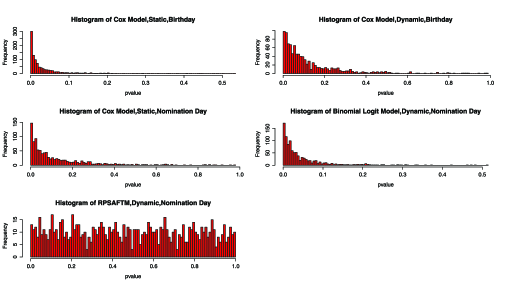
Figure 3: Histograms for $p$-values from the test of whether winning has an effect on mortality based on the four methods of previous studies and the RPSAFTM introduced by the current paper.

Table 12: Simulation results

Type of analysis	Status	Time-zero	Mean of $\bolds{p}$-value
PH	Static	Birthday	0.03
PH	Dynamic	Birthday	0.12
PH	Dynamic	Nomination day	0.12
PY	Dynamic	Nomination day	0.04
RPSAFTM	Dynamic	Nomination day	0.49

Figure 3 contains histograms for $p$-values of the five methods from 1000 simulations.

In the first four plots, the majority of the $p$-values are smaller than 0.2, while in the last plot, the $p$-values are uniformly distributed. The RPSAFTM corrects the survivor treatment selection bias that previous methods suffer from.

4 Analysis of Oscar Award data

We have compiled a data file that records the nominees and winners for each award (best lead actor, best lead actress, best supporting actor, best supporting actress) on each Oscar Award date. We collected the data from www.imdb.com. The data is in the supplementary materials [Han et al. (2010)]. The selection interval spanned from the inception of the Oscar Awards to July 25, 2007. In computing lifetime since being nominated, we use the actual Oscar Award date which varies from year to year. People who were not reported dead on www.imdb.com were presumed to be alive. There are 260 winners and 564 nonwinning nominees, 824 performers in all. Of these 824 performers, 448 are censored.

We did not include several candidates in our data set. Margaret Avery was nominated for best supporting actress in 1985, but we could not find her birthday and day of death from the internet. We did not include the following candidates who died before the winner of the award for which they were nominated was announced: Massimo Troisi, Jeanne Eagels, James Dean, Spencer Tracy, Peter Finch, and Ralph Richardson.

We have shown results from previous studies, which are based on less years of Oscar data than ours, in Table 1. To compare previous studies with ours, we have applied the methods of previous studies to our updated Oscar Award data set; the results are shown in Table 13. Compared with the results in Table 1, the reductions in mortality rate in Table 13 are smaller. The confidence intervals are also narrower, because we have 7 years more candidates than the original data set, and also each candidate in our data set has 7 years more information.

Table 13: Winners vs. nominees

			Reduction in
			mortality rate
Type of analysis	Status	Time-zero	(95% CI) (%)
PH	Static	Birthday	19 (6 to 31)0.0..0$-$
PH	Dynamic	Birthday	09 ($-$6 to 22)0.0..0
PH	Dynamic	Nomination day	14 (0 to 26)0.0..0$-$
PY	Dynamic	Nomination day	10 ($-$6 to 23)0.0..0
PH2	Dynamic	Nomination day	08.7 ($-$7.3 to 24.7)

In Table 8 the first four rows are based on previous methods. We also add the fifth row, which corresponds to a Cox time-dependent model adjusting for past nomination history and winning history; nomination history is adjusted for by conditioning on the number of previous nominations. Note that previous methods did not consider the nomination history.

We now consider fitting the RPSAFTM. For the conditional logistic regression (3.3), we use the following time dependent covariates $W_{ij}$: age of nomination (nomage), square of age of nomination (nomage.square), cube of age of nomination (nomage.cubic), and number of previous nominations (numprenom). Table 14 shows the results of the conditional logistic regression model (3.3) when $\psi=0$.

Table 14: Summary of conditional logistic model

	coef	$\mathbf{exp}$(coef)	se(coef)	$\bolds{z}$	$\bolds{p}$-value
$U_{ij}^{**}(0)$	$-$$1.37e{-}$02	1.01	$0.007541$	$-$1.812	0.07
nomage	$-$$5.36e{-}$02	1.06	$0.101676$	$-$0.527	0.60
nomage.square	$-9.18e{-}$04	1.00	$0.002278$	$-$0.403	0.69
nomage.cubic	$-$$7.40e{-}$06	1.00	$0.000016$	$-$0.462	0.64
numprenom	$-$$6.99e{-}$02	1.07	$0.071407$	$-$0.979	0.33

The $p$-value for the test of whether the coefficient on $U_{ij}^{**}(0)$ is 0, that is, the test of $H_{20}\dvtx\theta(0)=0$ vs. $H_{2a}\dvtx\theta(0)\neq 0$, is 0.07. Thus, we do not reject the null hypothesis that winning an Oscar has no effect on a performer’s survival at the 0.05 level. Looking at the effect of the other covariates (the $W_{ij}$) in Table 14, there is not strong evidence that number of previous nominations has an effect on the probability of a performer winning. For age at time of nomination, although the $p$-values on each of the polynomial terms are not significant, a test that the coefficient on all three of the terms is zero gives a $p$-value of 0.03 so age at time of nomination does appear to affect winning. Older nominees are slightly more likely to win.

The validity of our test of the effect of winning an Oscar depends critically on correctly controlling for the effect of age at time of nomination on winning since this age is clearly correlated with $U_{ij}$ (older nominees generally live a shorter time after the award date, so have smaller $U_{ij}$’s). To check that our results are robust to different ways of controlling for age at time of nomination, we replaced the cubic polynomial in nomage in Table 10 with a cubic spline of nomage with 1 to 4 knots placed at equally spaced quantiles. The $p$-values for the test of $H_{20}\dvtx\theta(0)=0$ vs. $H_{2a}\dvtx\theta(0)\neq 0$ ranged from 0.064 to 0.07 in these analyses. Thus, our result that there is not evidence that winning has an effect on survival at the 0.05 level is robust to how nomage is controlled for. We will use the cubic polynomial for nomage in Table 14 in our subsequent discussion.

Table 15 shows the $95\%$ confidence interval for the treatment effect. Our $95\%$ confidence interval is that the effect of winning is in the range of decreasing survival (after the award date) by $0.88\%$ to increasing survival by $26.62\%$.

=185pt Treatment effect CI $\psi$ $[-0.2360,0.0088]$ Winning multiplies survival $\exp(-\psi)$ $[0.9912,1.2662]$

Table 15: $95\%$ confidence interval for treatment effect

Robins’ $g$-estimate for the treatment effect is the $\psi_{0}$ that makes $\widehat{\theta}(\psi_{0})=0$ in the conditional logistic regression (3.3). This $\psi_{0}$ maximizes the $p$-value for testing $H_{20}\dvtx\theta(\psi_{0})=0$ vs. $H_{2a}\dvtx\theta(\psi_{0})\neq 0$. Robins et al. (1992) show that the $g$-estimate is asymptotically normal and consistent. The $g$-estimate can also be viewed as the Hodges–Lehmann (1963) estimate of the treatment effect based on the test of $H_{20}\dvtx\theta(\psi_{0})=0$.

We search for possible values of $\psi_{0}$ with $\widehat{\theta}(\psi_{0})=0$ in the range $[-0.2360,\break 0.0088]$ with step size${}=0.0001$. Figure 4 shows the estimates $\widehat{\theta}(\psi_{0})$ and the $p$-values for testing $H_{20}\dvtx\theta(\psi_{0})=0$. $\widehat{\theta}(\psi)$ is a monotone increasing function of $\psi$ in $[-0.2360,0.0088]$. The $g$-estimate is $\widehat{\psi}=-0.1127$, which corresponds to winning increasing survival by $12\%$.

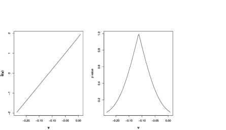
Figure 4: Estimate of the coefficient $\theta$ of the modified potential failure time variable $U_{ij}^{**}(\psi)$ in the conditional logistic regression (3.3) for different treatment effect value $\psi$ and $p$-values from the test of whether $\theta(\psi)$ equal zero for different $\psi$.

To estimate the survival advantage for winners in terms of years, we consider the performers who won the first time they were nominated. For these performers, we find their censored latent failure time $U_{ij}^{**}(\widehat{\psi})$ under the assumption that the point estimate $\widehat{\psi}$ of $\psi$ is the true treatment effect. Then we make Kaplan–Meier estimates for the distribution of the actual survival times for these winners and for the distribution of the latent survival times if these winners had never won. The difference between the estimated medians of these two distributions is an estimate of the survival advantage of winning the award for these winners. In the current Oscar Award data, we estimate the survival advantage to be 4.2 years, with a $95\%$ confidence interval of $[-0.4,8.4]$ years.

4.1 Diagnostic plots

To examine whether the RPSAFTM is appropriate for the Oscar Award data set, we use boxplots to check if the randomization assumption (Assumption 1) is violated for latent failure times computed according to the RPSAFTM at our point estimate $\widehat{\psi}$ of $\psi$. This is similar to the diagnostics for testing an additive treatment effect model in Small et al. (2006). Based on the randomization assumption, for the point estimate $\widehat{\psi}$, the distributions of $U_{ij}^{**}(\widehat{\psi})$ should be approximately the same for the treatment group (winners) and the control group (nonwinning nominees) in the same range of nomage. We divide the candidates into five subgroups based on the quantiles of nomage. For each subgroup, we make boxplots for $U_{ij}^{**}(\widehat{\psi})$ for the winners and the nonwinning nominees.

Figure 5: Boxplots of $U_{ij}^{**}(\widehat{\psi})$ for comparison between treatment group (winners) and control group (nonwinning nominees) in five subgroups based on the quantiles of nomage.

Figure 5 shows the distribution of $U_{ij}^{**}(\widehat{\psi})$ is similar among winners and nonwinning nominees for each range of nomage. This supports the validity of the RPSAFTM (assuming that Assumption 1 is valid).

4.2 Sensitivity analysis

Our basic assumption, Assumption 1, is that, conditional on covariates such as age at nomination, and number of previous nominations, who wins the Oscar Award is not related to how long the candidates would have lived without winning an award. This could be violated if performers who lead a more healthy lifestyle are more likely to win or if performers who lead a more reckless lifestyle are more likely to win. We now provide a sensitivity analysis to violations of Assumption 1. Under Assumption 1, $\theta(\psi)$ is 0. If Assumption 1 is violated, then $\theta(\psi)=\theta^{*}\neq 0$. For $\theta(\psi)=\theta^{*}$, we can test the plausibility of $\psi_{0}$ by testing $H_{20}^{\prime}\dvtx\theta(\psi_{0})=\theta^{*}$ vs. $H_{2a}^{\prime}\dvtx\theta(\psi_{0})\neq\theta^{*}$. To calibrate $\theta^{*}$, we note that we can interpret $\exp(10\theta^{*})$ as the odds ratio for one candidate to win compared to another, if the one candidate has a ten year higher latent failure time than the other and the two candidates are the same age at nomination and have the same number of previous nominations. Under Assumption 1, $\exp(10\theta^{*})=1$. Table 16 shows confidence intervals for $\psi$ and the survival advantage of winning for winners at first nomination for different values of $\theta^{*}$.

Table 16: Sensitivity analysis

$\mathbf{exp}\!\bolds{(10\theta^{*})=}$
Odds ratio for two			Survival advantage
otherwise equal people			in terms of years
one has 10 years			point estimate/
higher $\bolds{U_{ij}^{**}}$ than other	$\bolds{\theta^{*}}$	Confidence interval for $\bolds{\psi}$	confidence interval
0.5	$-$0.0693	$(-0.6587,-0.4174)$	$16.4/(13.6,19.3)$
0.6	$-$0.0511	$(-0.5652,-0.3235)$	$14.1/(11.0,17.2)$
0.7	$-$0.0357	$(-0.4769,-0.2374)$	$11.7/(8.4,15.1)$
0.8	$-$0.0223	$(-0.3911,-0.1550)$	$9.3/(5.7,12.9)$
0.9	$-$0.0105	$(-0.3100,-0.0730)$	$6.8/(2.8,10.6)$
10.	$-$0.0000	$(-0.2360,0.0088)$	$4.2/(-0.4,8.4)$
1.1	$-$0.0095	$(-0.1654,0.0879)$	$1.4/(-3.7,6.1)$
1.2	$-$0.0182	$(-0.0940,0.1697)$	$-1.5/(-6.9,3.6)$
1.3	$-$0.0262	$(-0.0210,0.2515)$	$-4.4/(-10.9,0.8)$
1.4	$-$0.0336	$(0.0413,0.3359)$	$-7/(-16.4,-1.3)$
1.5	$-$0.0405	$(0.0985,0.4238)$	$-10.3/(-19.2,-4.2)$

As the odds ratio $\exp(10\theta^{*})$ increases from 0.5 to 1.5, the point estimate of the survival advantage decreases from 16.4 years to $-$10.3 years. If less healthy candidates are moderately more likely to win than healthy candidates, $\exp(10\theta^{*})=0.9$, then the confidence interval only contains negative $\psi$, and there is strong evidence that winning increases survival. But if more healthy candidates are somewhat more likely to win than less healthy candidates, $\exp(10\theta^{*})=1.2$, then the confidence interval contains predominantly positive $\psi$ and the point estimate is that winning decreases survival.

5 Discussion

In this paper we point out that healthy performer survivor bias exists in methods from previous studies of the effect of winning an Oscar on survival. We show that under Assumption 1 (among nominees, the winner is randomly selected conditional on baseline covariates), Robins’ RPSAFTM eliminates healthy performer survivor bias. We estimated that the effect of winning an Oscar Award on survival for winners at first nomination is to increase survival by 4.2 years, but the $95\%$ confidence interval of $[-0.4,8.4]$ years contains negative effects. Thus, our study indicates that there is not strong evidence that winning an Oscar increases life expectancy.

The analysis in this paper is a case study of how Robins’ RPSAFTM can provide an improvement over Cox proportional hazards models for estimating the effect on survival of a sudden change in a person’s life, for example, becoming ill, starting a high risk behavior, or starting a treatment. A key assumption (our Assumption 1) that is needed to obtain inferences from the RPSAFTM is that, conditional on covariates recorded up to a given time, the sudden change is “randomly” assigned. A feature of our application, unlike most other applications of RPSAFTMs [e.g., Robins et al. (1992); Hernán et al. (2005)], is that we only assume the sudden change is randomly assigned among a select subset of the people in the study rather than all people in the study. In particular, we are only assuming that among nominees in a given year, who are generally at least somewhat healthy in the given year, the winner is randomly selected. We are not assuming that the winner is randomly selected from the pool of all actors and actresses who have been nominated in a previous year or the given year and are still alive. Some performers nominated in a previous year might be too unhealthy to act even though they are still alive. Similar consideration of comparability only among a selected subset can be found in Joffe et al. (1998) and Robins (2008).

In the RPSAFTM, model (1) is rank preserving, that is, the effect of winning is the same for each subject. Robins et al. (1992) and Lok et al. (2004) discussed an expanded class of SAFTMs, which does not need the RHS of (1) at the true $\psi$ to be equal to the actual counterfactual failure time $U_{ij}$, rather it just needs that the RHS and the $U_{ij}$ have the same distribution conditional on past measured covariates sufficient to control confounding. This eliminates the assumption of rank preservation without changing the method of estimation of the population (i.e., distributional) interpretation of $\psi$.

References

- (1) Abel, E. L. and Kruger, M. L. (2005). The longevity of Baseball hall of famers compared to other players. Death Studies 29 959–963.
- (2) Cox, D. R. and Oakes, D. (1984). Analysis of Survival Data. Chapman and Hall, London. \MR0751780
- (3) Efron, B. (2002). The two-way proportional hazards model. J. R. Stat. Soc. Ser. B Stat. Methodol. 64 899–909. \MR1979394
- (4) Ferrie, J. E., Shipley, M. J., Davey, S. G., Stansfeld, S. A. and Marmot, M. G. (2002). Change in health inequalities among British civil servants: The Whitehall II study. Journal of Epidemiology and Communitiy Health 56 922–926.
- (5) Gehrlein, W. V. and Kher, H. V. (2004). Decision rules for the Academy Awards versus those for elections. Interfaces 34 226–234.
- (6) Han, X., Small, D., Foster, D. and Patel, V. (2010). Supplement to “The effect of winning an Oscar Award on survival: Correcting for healthy performer survivor bias with a rank preserving structural accelerated failure time model.” DOI: 10.1214/10-AOAS424SUPPA, DOI: 10.1214/10-AOAS424SUPPB.
- (7) Hernán, M. A., Cole, S. R., Margolick, J. B., Cohen, M. H. and Robins, J. M. (2005). Structural accelerated failure time models for survival analysis in studies with time-varying treatments. Pharmacoepidemiology and Drug Safety 14 477–491.
- (8) Hodges, J. L. and Lehmann, E. L. (1963). Estimates of location based on rank tests. Ann. Math. Statist. 34 598–611. \MR0152070
- (9) Joffe, M. M., Hoover, D. R., Jacobson, L. P., Kingsley, L., Chmiel, J. S., Visscher, B. R. and Robins, J. M. (1998). Estimating the effect of zidovudine on Kaposi’s Sarcoma from observational data using a rank preserving structural failure-time model. Stat. Med. 17 1073–1102.
- (10) Lok, J., Gill, R., Van Der Vaart, A. and Robins, J. (2004). Estimating the causal effect of a time-varying treatment on time-to-event using structural nested failure time models. Statist. Neerlandica 58 271–295. \MR2157006
- (11) Marmot, M. G., Davey, S. G., Stansfeld, S., Patel, C., North, F., Head, J., White, I., Brunner, E. and Feeney, A. (1991). Health inequalities among British civil servants: The Whitehall II study. Lancet 337 1387–1393.
- (12) Marmot, M. G., Rose, G. and Hamilton, P. J. S. (1978). Employment grade and coronary heart disease in British civil servants. Journal of Epidemiology and Community Health 32 244–249.
- (13) Marmot, M. G., Shipley, M. J. and Rose, G. (1984). Inequalities in death—specific explanations of a general pattern? Lancet 323 1003–1006.
- (14) McFadden, D. (1974). Conditional logit analysis of qualitative choice behavior. In Frontiers in Econometrics (P. Zarembka, ed.) 105–142. Academic Press, New York.
- (15) Rablen, M. D. and Oswald, A. J. (2008). Mortality and immortality: The Nobel Prize as an experiment into the effect of status upon longevity. Journal of Health Economics 27 1462–1471.
- (16) Redelmeier, D. A. and Singh, S. M. (2001). Survival in Academy Award—winning actors and actresses. Ann. Intern. Med. 134 955–962.
- (17) Reid, D. D., Brett, G. Z., Hamilton, P. J. S., Jarrett, R. J., Keen, H. and Rose, G. (1974). Cardio-respiratory disease and diabetes among middle-aged male civil servants: A study of screening and intervention. Lancet 303 469–473.
- (18) Robins, J. M. (1986). A new approach to causal inference in mortality studies with a sustained exposure period—applications to control of the healthy worker survivor effect. Math. Model. 7 1393–1512. \MR0877758
- (19) Robins, J. M. (1992). Estimation of the time-dependent accelerated failure time model in the presence of confounding factors. Biometrika 79 321–334. \MR1185134
- (20) Robins, J. M. (1993). Analytic methods for estimating HIV treatment and cofactor effects. In Methodological Issues of AIDS Mental Health Research 213–290. Plenum Publishing, New York.
- (21) Robins, J. M. (2008). Causal models for estimating the effects of weight gain on mortality. International Journal of Obesity 32 S15–S41.
- (22) Robins, J. M., Blevins, D., Ritter, G. and Wulfson, M. (1992). -estimation of the effect of prophylaxis therapy for pneumocystis carinii pneumonia on the survival of AIDS patients. Epidemiology 3 319–336.
- (23) Sapolsky, R. (2005). The influence of social hierarchy on primate health. Science 308 648–652.
- (24) Small, D., Gastwirth, J., Krieger, A. and Rosenbaum, P. (2006). R-estimates vs. GMM: A theoretical case study of validity and efficiency. Statist. Sci. 21 363–375. \MR2339136
- (25) Sylvestre, M. P., Huszti, E. and Hanley, J. A. (2006). Do Oscar winners live longer than less successful peers? A reanalysis of the evidence. Ann. Intern. Med. 145 361–363.