Graphene in periodically alternating magnetic field: unusual quantization of the anomalous Hall effect

Abstract

We study the energy spectrum and electronic properties of graphene in a periodic magnetic field of zero average with a symmetry of triangular lattice. The periodic field leads to formation of a set of minibands separated by gaps, which can be manipulated by external field. The Berry phase, related to the motion of electrons in $k$ space, and the corresponding Chern numbers characterizing topology of the energy bands are calculated analytically and numerically. In this connection, we discuss the anomalous Hall effect in the insulating state, when the Fermi level is located in the minigap. The results of calculations show that in the model of gapless Dirac spectrum of graphene the anomalous Hall effect can be treated as a sum of fractional quantum numbers, related to the nonequivalent Dirac points.

I Introduction

The energy structure of graphene includes the Dirac points where the energy spectrum of electrons is relativistic. This can lead to many very unusual transport properties of this material novoselov04 ; novoselov05 ; geim07 ; neto09 ; peres10 . One of examples is the unusual integer quantum Hall effect in graphene. As found theoretically and confirmed experimentally novoselov05 ; zhang05 there is no $N=0$ plateau, which is related to the Dirac point in the electronic spectrum. The other very important property is that the Landau splitting is very strong in graphene, which makes it possible to observe the quantum Hall effect at room temperatures novoselov07 .

Recently, we proposed to use a periodic magnetic field for quantization of the electron energy spectrum of two-dimensional electron gas taillefumier08 . Our calculations demonstrated that periodically alternating field leads to an energy spectrum with a number of minibands separated by energy gaps. In such system, the anomalous Hall effect (AHE) is nonzero, and it is quantized if the chemical potential is located within the gap. It was also suggested bruno04 ; taillefumier08 that the realization of such structure under periodic magnetic field can be easily achieved by using a lattice of magnetic nanorods nielsch01 . It should be noted that another possible way is to use the 2D skyrmion lattice rossler06 , which have been recently observed in thin layers of helical magnets (however, in this case the temperature should be rather low) yu10 .

Graphene has obvious advantages to be used instead of semiconducting quantum well with two-dimensional electron spectrum. Graphene is naturally two-dimensional, and the technology of graphene-based structures is much simpler. Besides, one can expect much stronger effects related to the magnetic quantization due to the specific parameters of graphene.

In this work we calculate the electron energy spectrum and the Chern numbers characterizing topological properties of the energy bands. The results are essentially different for graphene as compare to the 2D electron gas with parabolic energy spectrum. We find that the Chern numbers of the bands corresponding to higher-in-energy excitations of electrons and holes are zero at sufficiently large field. On the contrary, the low-energy bands of electrons and holes have nonzero Chern numbers, which results in the quantized anomalous Hall effect.

II Generalized model with the gap

We start with a generalized model, which includes the relativistic Hamiltonian neto09 describing the electron energy spectrum near the Dirac points $\mathcal{K,\,K^{\prime}}$ in the Brillouin zone of graphene (Fig. 1a) and an additional term leading to the gap

$$\mathcal{H}^{\mathcal{K,\,K^{\prime}}}=\mp iv\tau_{x}\left(\partial_{x}-\frac{ieA_{x}}{c}\right)-iv\tau_{y}\left(\partial_{y}-\frac{ieA_{y}}{c}\right)$$

$$+\Delta\tau_{z},$$ (1)

where the components of vector $\tau$ are the Pauli matrices acting in the space of graphene sublattices. Introducing the gap parameter $\Delta$ makes the A and B sites different in the crystal lattice of graphene. Physically, it can be the case of different atoms in the honeycomb lattice like in two-dimensional boron nitride. The model with $\Delta\neq 0$ can be also realized for graphene in periodic electric and magnetic fields discussed in Ref. [snyman09, ]. In the case of graphene we should put $\Delta=0$ but for pedagogical reasons it is instructive to start from $\Delta\neq 0$. The vector potential ${\bf A}({\bf r})$ describes the effect of magnetic field.

We assume that the graphene sheet is in the periodically alternating magnetic field in $z$ direction. In our analytical calculations we consider one-harmonic approach, $B({\bf r})=(B_{0}/3)\,{\rm Re}\sum_{i=1}^{3}e^{i{\bf g}_{i}\cdot{\bf r}}$, where the in-plane vectors ${\bf g}_{i}$ can be viewed as basic vectors of the triangular lattice. In the numerical calculations we include more harmonics to make the consideration realistic, preserving the triangular symmetry of the field-imposed lattice. One can use the gauge in which the correspondent vector potential is also periodic, ${\bf A}({\bf r})={\rm Im}\sum_{i}{\bf a}_{i}\,e^{i{\bf g}_{i}\cdot{\bf r}}$, where ${\bf a}_{i}=(B_{0}/3g_{i}^{2})\,({\bf n}_{0}\times{\bf g}_{i})$ and ${\bf n}_{0}$ is the unit vector along axis $z$ perpendicular to the plane.

We also assume that the period $a$ of alternating field is much much larger than the lattice constant of graphene $a_{0}$. The large scale field-induced triangular lattice determines the corresponding small Brillouin zone in the inverse space (Fig. 1b), and we denote the symmetry points of this zone by $K$, $M$, etc. It should be stressed that these points are not related in any way to the symmetry points of the Brillouin zone of graphene, which we denote like $\mathcal{K}$ and $\mathcal{K}^{\prime}$ (Fig. 1).

III Perturbation theory

Let us assume $\Delta$ very small and positive, $\Delta>0$. In the case of weak periodic field, the term with ${\bf A}({\bf r})$ in (1) is a weak perturbation. We consider first the states related to the Dirac point $\mathcal{K}$. For ${\bf A}=0$, the unperturbed solution for the low-energy state in the $\Gamma$ point with $\varepsilon>0$ is

$$\psi^{(0)}_{\Gamma,+1}({\bf r})=\frac{1}{\sqrt{\mathcal{S}}}\,\left(\begin{array}[]{c}1\\ 0\end{array}\right),\hskip 5.69046pt\psi^{(0)}_{\Gamma,-1}({\bf r})=\frac{1}{\sqrt{\mathcal{S}}}\,\left(\begin{array}[]{c}0\\ 1\end{array}\right),$$ (6)

where $\mathcal{S}$ the sample surface, and index $\pm 1$ refers to the states in the first low-energy energy band with positive and negative energy, respectively. Assuming $\Delta$ very small, for any other point $k\neq 0$ the solution is

$$\psi^{(0)}_{{\bf k},\pm 1}({\bf r})\simeq\frac{e^{i{\bf k}\cdot{\bf r}}}{\sqrt{2\mathcal{S}}}\left(\begin{array}[]{c}1\\ \pm(k_{x}+ik_{y})/k\end{array}\right),$$ (9)

corresponding to the states with energy $\varepsilon_{{\bf k},\pm 1}\simeq\pm vk$.

The Hamiltonian of interaction is $\mathcal{H}_{int}=-\frac{ev}{c}\,\mbox{\boldmath$\tau$}\cdot{\bf A}$. Matrix elements of the periodic field between the states $\psi^{(0)}_{{\bf k}\alpha}$ and $\psi^{(0)}_{{\bf k^{\prime}}\beta}$ are nonzero only for ${\bf k}-{\bf k^{\prime}}={\bf g}$, where ${\bf g}$ is one of the vectors $\pm{\bf g}_{1}$, $\pm{\bf g}_{2}$, $\pm{\bf g}_{3}$. Correspondingly, the weak periodic field mostly affects the states at the Brillouin zone edge, which have close in energy counterparts, $\varepsilon^{(0)}_{{\bf k}\alpha}\simeq\varepsilon^{(0)}_{{\bf k}-{\bf g}_{i},\alpha}$. Then for the state at the $\Gamma$ point $\psi_{\Gamma}({\bf r})\simeq\psi_{\Gamma}^{(0)}({\bf r})$, whereas the wave functions near the points $M$ and $K$ of reciprocal lattice can be presented as a superposition of unperturbed functions, $\psi_{\bf k}({\bf r})=c_{0}\psi^{(0)}_{\bf k}({\bf r})+\sum_{i}c_{i}\psi^{(0)}_{{\bf k}-{\bf g}_{i}}({\bf r})$.

For the lower-in-energy states with $\varepsilon>0$ in $M$ and $K$ points we find

$$\psi_{M,+1}({\bf r})\simeq\frac{e^{i{\bf k}_{M}\cdot{\bf r}}}{2\sqrt{\mathcal{S}}}\left[\left(\begin{array}[]{c}1\\ 1\end{array}\right)+e^{-i{\bf g}_{3}\cdot{\bf r}}\left(\begin{array}[]{c}1\\ -1\end{array}\right)\right].$$ (14)

$$\psi_{K,+1}({\bf r})\simeq\frac{e^{i{\bf k}_{K}\cdot{\bf r}}}{\sqrt{6\mathcal{S}}}\left[\left(\begin{array}[]{c}1\\ \frac{\sqrt{3}+i}{2}\end{array}\right)+e^{-i{\bf g}_{2}\cdot{\bf r}}\left(\begin{array}[]{c}1\\ -i\end{array}\right)\right.$$ (19)

$$\left.+e^{-i{\bf g}_{3}\cdot{\bf r}}\left(\begin{array}[]{c}1\\ \frac{-\sqrt{3}+i}{2}\end{array}\right)\right].$$ (22)

Using these functions we calculate the Berry phase $\gamma_{C}$ along the contour $\Gamma$-$M$-$K$-$\Gamma$, shown in Fig. 1b, as

$$\gamma_{C}=\arg\left<\Gamma|M\right>\left<M|K\right>\left<K|\Gamma\right>=0,$$ (23)

Thus, for the contour along the whole Brillouin zone and the first energy band we obtain $\gamma_{+1}=12\gamma_{C}=0$. Correspondingly, the Chern number of the $(+1)$ band is ${\rm Ch}_{+1}=\gamma_{+1}/2\pi=0$. Using the same method for the negative energy band $(-1)$, we find $\gamma_{-1}=-2\pi$ and ${\rm Ch}_{-1}=-1$.

Figure 1: (a) Brillouin zone of graphene with two nonequivalent Dirac points; (b) Brillouin zone corresponding to a single Dirac point of graphene in a large-scale periodic field of triangular symmetry. Contour $\gamma_{c}$ in the $k$-space.

We should also take into account the contribution of the another non-equivalent Dirac point $\mathcal{K}^{\prime}$. For this point the Hamiltonian (1) differs by the opposite sign before $\partial_{x}$ and $A_{x}$. Calculating the wavefunctions in this case and using (6) we can find for the positive energy band ${\rm Ch}_{+1}=-1$ and for negative band ${\rm Ch}_{-1}=0$.

If we take $\Delta<0$, we obtain for the $\mathcal{K}$ point ${\rm Ch}_{+1}=-1$ and ${\rm Ch}_{-1}=0$. Correspondingly, for the $\mathcal{K}^{\prime}$ point the results are ${\rm Ch}_{+1}=0$ and ${\rm Ch}_{-1}=-1$.

IV Symmetry arguments

These results can be understood using the symmetry of Hamiltonian (1). Indeed, the transition from $\mathcal{K}$ to $\mathcal{K}^{\prime}$ with simultaneous reversion of the sign of $\Delta$ is related to the symmetry under the unitary transformation (rotation in sublattice space)

$$\tau_{y}^{-1}\mathcal{H}^{\mathcal{K}}(\Delta)\tau_{y}=\mathcal{H}^{\mathcal{K}^{\prime}}(-\Delta).$$ (24)

Such transformation applied to the wavefunctions does not change the Berry phase (6). Therefore, the corresponding Chern numbers should be equal,

$${\rm Ch}_{n}(\mathcal{K},\Delta)={\rm Ch}_{n}(\mathcal{K}^{\prime},-\Delta).$$ (25)

Besides, changing the sign of field (i.e., ${\bf A}\to-{\bf A}$) in (1) with simultaneous spatial inversion and reversion of the sign of $\Delta$ is equivalent to the change of sign of Hamiltonian

$$\mathcal{H}({\bf r},{\bf A},\Delta)=-\mathcal{H}(-{\bf r},-{\bf A},-\Delta),$$ (26)

which corresponds to the electron-hole symmetry. It can be also understood as a symmetry to the pseudotime inversion, $\tilde{T}=i\tau_{y}\mathcal{R}$, where $\mathcal{R}$ is the complex conjugation operator

$$\tilde{T}^{-1}\mathcal{H}({\bf A},\Delta)\tilde{T}=\mathcal{H}(-{\bf A},-\Delta).$$ (27)

The complex conjugation operator acting on the wavefunctions changes the sign of the Berry phase, and we obtain

$${\rm Ch}_{n}({\bf A},\Delta)=-{\rm Ch}_{n}(-{\bf A},-\Delta).$$ (28)

Also, there is a symmetry with respect to $\tau_{z}$ transformation:

$$\tau_{z}^{-1}\mathcal{H}(\Delta)\,\tau_{z}=-\mathcal{H}(-\Delta)$$ (29)

leading to ${\rm Ch}_{n}(\Delta)={\rm Ch}_{-n}(-\Delta)$.

Using these properties, we can analyze what happens when the parameter $\Delta$ changes sign from negative to positive. It will helps us to determine properly the AHE for the case of $\Delta=0$.

V Anomalous Hall effect

We start from relation between the Chern numbers and AHE. For the contribution of points $\mathcal{K,K^{\prime}}$ to the off-diagonal conductivity, in the case when the chemical potential $\mu$ is in the gap, one can use the standard formula nagaosa10

$$\sigma_{xy}=\frac{e^{2}}{\hbar}\sum_{{\bf k}n}f(\varepsilon_{{\bf k}n})\Omega_{{\bf k}n},$$ (30)

where $f(\varepsilon)$ is the Fermi-Dirac distribution function, $\Omega_{{\bf k}n}=\nabla_{\bf k}\times\mbox{\boldmath$\mathcal{A}$}_{{\bf k}n}$ is the Berry curvature, and $\mbox{\boldmath$\mathcal{A}$}_{{\bf k}n}=-i\langle{\bf k}n|\nabla_{\bf k}|{\bf k}n\rangle$ is the gauge connection. The energy spectrum is shown in Fig. 2 for different values of magnetic field (the discussion is in Sec. VII).

The sum over $n$ in Eq. (13) formally includes infinite number of energy bands with negative energies of electrons. However, one can show that in the model of Eq. (1) the contribution of all the bands with $\varepsilon_{{\bf k}n}<0$ to the AHE is equal to zero. The reason is that if we take $\Delta\neq 0$ and the chemical potential $\mu=0$ than the sum of Chern numbers for the $\mathcal{K}$ and $\mathcal{K}^{\prime}$ Dirac points does not change with changing periodic field from $B({\bf r})$ to $-B({\bf r})$. Indeed, any gradual variation of the field amplitude from $B_{0}$ to $-B_{0}$ does not change the Chern numbers because, as one can see from the band structure calculations, this does not produce any field-induced band crossings. This does not depend on the value and sign of $\Delta$ and therefore is also valid in the limit of $\Delta\to 0$. Since the sum of Chern numbers and the resulting AHE at $\mu=0$ is invariant with respect to field inversion, then, due to the antisymmetry of AHE to the field, it should be zero. Thus, in the vacuum state with $\mu=0$ there is no Hall effect in graphene.

If the chemical potential $\mu\neq 0$ and is located somewhere within the gap, the AHE is not necessary zero and can be calculated from the following formula, which gives the quantized values of the Hall conductivity

$$\sigma_{xy}=\frac{e^{2}}{h}\left({\sum_{n}}^{\prime}\text{Ch}_{n}-\sum_{n<0}\text{Ch}_{n}\right).$$ (31)

Here ${\rm Ch}_{n}=\frac{1}{2\pi}\int d^{2}{\bf k}\;\Omega_{{\bf k}n}$ is the Chern number of the $n$-th energy band, and the first sum in (14) runs over the occupied energy bands.

Using the obtained results for the Chern numbers we find that the contribution from the $\mathcal{K}$ point changes (in units of $e^{2}/h$) from $-1$ to 0 when the parameter $\Delta$ changes from negative to positive values. Similarly, the contribution from the $\mathcal{K}^{\prime}$ switches from 0 to $-1$ when $\Delta$ changes from $\Delta<0$ to $\Delta>0$. The sum of contributions from both $\mathcal{K}$ and $\mathcal{K}^{\prime}$ is equal to $-1$ for any sign of $\Delta$, and the sign of $\Delta$ determines, which of the points $\mathcal{K}$ or $\mathcal{K}^{\prime}$ is contributing to the AHE. But in the point of $\Delta=0$, which corresponds to the gapless model of graphene, the contributions from $\mathcal{K}$ and $\mathcal{K}^{\prime}$ are exactly the same. Therefore, we come to conclusion that at $\Delta=0$ each of these points gives the fractional value of quantized Hall conductivity equal to $-1/2$.

VI Gapless Dirac model

Let us consider now the Hamiltonian (1) with $\Delta=0$. It has the symmetry $\tau_{z}^{-1}\mathcal{H}\tau_{z}=-\mathcal{H}$, which means that if $\psi_{n}$ is the eigenfunction of $\mathcal{H}$ with energy $\varepsilon_{n}$ then $\tau_{z}\psi_{n}$ corresponds to the state with energy $-\varepsilon_{n}$. The $\tau_{z}$ symmetry also means that the Berry phase calculated for any positive $(+n)$-band is exactly the same as for the $(-n)$ band.

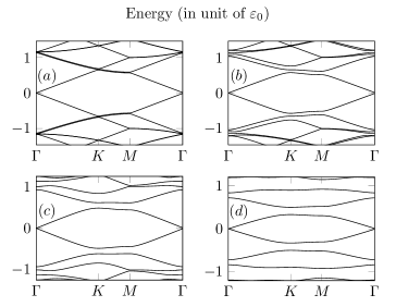
Figure 2: The electron band structure of graphene ($\Delta=0$) for different intensities of the field: (a) $\alpha=0.05$, (b) $\alpha=0.2$, (c) $\alpha=0.5$, (d) $\alpha=1.0$.

For any ${\bf k}$-point including $\Gamma$ we use the unperturbed wave functions (3). One can calculate the Berry phase $\gamma_{C}$ along the contour of Fig. 1b, excluding the $\Gamma$ point and using

$$\gamma_{C}=\arg\left<\Gamma|M\right>\left<M|K\right>\left<K|\Gamma^{\prime}\right>\left<\Gamma^{\prime}|\Gamma\right>,$$ (32)

where $\Gamma$ and $\Gamma^{\prime}$ correspond to the states with ${\bf k}\simeq 0$ along the $\Gamma$-$M$ and $\Gamma$-$K$ lines, respectively. It gives us for the $\mathcal{K}$ point and $\varepsilon>0$, $\gamma_{C}=-\pi/12$. The contour around the Brillouin zone gives us $\gamma_{+1}=12\gamma_{C}+\gamma_{0}$, where $\gamma_{0}$ is the Berry phase for a small contour around the $\Gamma$ point. The calculation gives $\gamma_{0}=\pi$. As a result we find the integer Chern number ${\rm Ch}_{+1}=0$. However, this Chern number does not determine the Hall conductivity corresponding to Eq. (14) because the contribution of $\gamma_{0}$ should be excluded from consideration as it does not depend on the external field. Thus, to calculate the AHE we should use the Berry phase without enclosing $\Gamma$ point, and we finally find that the contribution to AHE from any of the $\mathcal{K}$ or $\mathcal{K}$ points is equal to $-1/2$ in accordance with what we found before.

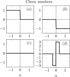
Figure 3: Numerically calculated Chern numbers of the first positive energy bands for small $\Delta\neq 0$ as a function of $\alpha$: (a) ${\rm Ch}_{+1}$ for $\Delta>0$, (b) ${\rm Ch}_{+1}$ for $\Delta<0$, (c) ${\rm Ch}_{+2}$, (d) ${\rm Ch}_{+3}$.

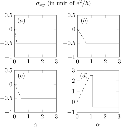
Figure 4: Hall conductivity per one spin and one valley as a function of magnetic field for different values of electron density: (a) $n_{0}=4$, (b) $n_{0}=8$, (c) $n_{0}=12$, (d) $n_{0}=16$, where $n_{0}$ is the total number of electrons per elementary cell of graphene in periodic field.

VII Numerical calculations

Using Hamiltonian (1) we performed numerical calculations of the energy band structure for different intensity of the periodic field. In these calculations we used the real numerically calculated distribution of magnetic field created by the lattice of magnetic nanorods, not restricting ourselves to harmonic approximation. The results are presented in Fig. 2 for different values of the dimensionless parameter of intensity of periodic field $\alpha$, defined as $\alpha=B_{0}a^{2}/4\pi\phi_{0}$, where $\phi_{0}$ is the flux quantum. Figure 2 demonstrates that the energy gap between the $(+1)$ and $(+2)$ bands appears at the field corresponding to $\alpha>0.2$.

We also calculated numerically the Chern numbers as a function of the field intensity. They are presented in Fig. 3 for the first three bands. It turns out that the results of perturbation theory for the low-energy bands $n=\pm 1$ remains valid with increasing $\alpha$. Figure 4 presents the Hall conductivity per one spin and one valley as a function of concentration of electrons. The dashed line corresponds to the unfilled energy band, where an additional contribution from the Fermi surface should be taken into account nagaosa10 but we do not consider this case.

VIII Estimation of parameters

The results of numerical calculations show that the first gap between the $(+1)$ and $(+2)$ bands appears at $\alpha>0.2$. In the case of iron nanorod lattice with a lattice parameter $a\simeq 150$ nm, we find that the magnitude of $B_{0}$ at a distance about 15 nm from the nanorod lattice is $B_{0}\simeq 0.2$ T taillefumier08 and that $\alpha\simeq 0.2$, which is in good agreement with the criteria of gap formation.

One can also estimate the electron density $n$ corresponding to the insulating state when the chemical potential $\mu$ is located in the first gap. This state is characterized by one electron per elementary cell, $n=4/\mathcal{S}_{0}$, where $\mathcal{S}_{0}=a^{2}\sqrt{3}/2$ and factor 4 takes into account degeneracy with respect to spin and valley in graphene. Using the relation $n=\mu^{2}/\pi v^{2}$, where $v/\hbar\simeq 1.5\times 10^{6}$ m/s is the electron velocity, we find $\mu\simeq 40$ meV. All necessary parameters are quite reachable for the technology of graphene.

One can estimate the characteristic energy $\varepsilon_{0}=hv/a\simeq 40$ meV for $a=150$ nm. From the band structure calculations we expect the gap to be of the order of $\varepsilon_{0}/6$. So, the gap is $\simeq 90$ K. For the Zeeman splitting in graphene we have $g\mu_{B}B_{0}\simeq 0.5$ K, so we expect that Zeeman splitting is negligibly small for this choice of parameters.

IX Discussion

We found that the AHE related to a single Dirac point in graphene is fractionally quantized, corresponding to quantum number $-1/2$. The quantization of AHE takes place if the chemical potential is located in the gap between the bands (+1) and (+2), which can be easily achieved with the existing experimental technique. The fractional quantization is related to the Dirac points, which is the monopole (for the $\mathcal{K}$ point) or antimonopole (for $\mathcal{K}^{\prime}$) in the ${\bf k}$ space, but the Berry phase related to these points does not contribute to the AHE. Correspondingly, the measured AHE in graphene with two nonequivalent Dirac points and two spin orientations is integer for the same parameters, $\sigma_{H}=ne^{2}/\hbar$ with $n=-2$.

Our consideration of the AHE is essentially based on the statement that in the clean case with $\mu=0$ the AHE is zero. In the above-studied model with $\Delta\neq 0$, it is related to the invariance of Hamiltonian and Chern numbers of the filled bands with respect to the inversion of field, which contradicts to antisymmetry of AHE. It does not depend on sign of $\Delta$ and leads to the zero vacuum AHE in the limiting case of $\Delta=0$ in graphene.

In this connection, it is important to compare our results with the result of Haldane’s model haldane88 , in which the AHE can be nonzero even in the vacuum state. In the Haldane’s model the periodic field has the same periodicity as the honeycomb lattice, and the model includes additional next-neighbor hoppings. Then the next-neighbor hopping integral in such a fast alternating field acquires nonzero phase factor, which leads to the brake of electron-hole symmetry. Obviously, this model is not invariant with respect to the field inversion, $B({\bf r})\to-B({\bf r})$. As a result, our arguments about vanishing of AHE in the ground state of graphene are not applicable to the model of Ref. [haldane88, ].

Figure 5: Brillouin zone and Berry sphere of the Haldane’s model in the case of $\Delta<3\sqrt{3}t_{2}\sin\phi$.

To clarify this point we reconsider the Haldane’s model by calculating the Hall conductivity as the Berry phase of electrons in the lower subband along the path encompassing the Brillouin zone of the honeycomb lattice. The Hamiltonian of Ref. [haldane88, ] can be presented as

$$\mathcal{H}_{H}=\varepsilon({\bf k})+\lambda\mbox{\boldmath$\sigma$}\cdot{\bf n}({\bf k})$$ (33)

where the unit vector ${\bf n}({\bf k})$ parametrizes $2\times 2$ pseudospin Hamiltonian. Here we denoted

$$\varepsilon({\bf k})=2t_{2}\cos\phi\sum_{i}\cos({\bf k}\cdot{\bf b}_{i}),$$ (34)

$$n_{x}({\bf k})=(t_{1}/\lambda)\sum_{i}\cos({\bf k}\cdot{\bf a}_{i}),$$ (35)

$$n_{y}({\bf k})=(t_{1}/\lambda)\sum_{i}\sin({\bf k}\cdot{\bf a}_{i}),$$ (36)

$$n_{z}({\bf k})=[\Delta-t_{2}\sin\phi\sum_{i}\sin({\bf k}\cdot{\bf b}_{i})]/\lambda,$$ (37)

where the lattice vectors ${\bf a}_{i}$ and ${\bf b}_{i}$ are defined in [haldane88, ] and the parameter $\lambda$ is introduced to provide $|{\bf n}|$=1. The parameter $t_{2}$ is the next-neighbor hopping integral and the phase $\phi$ is due to this hopping in the field with the periodicity of crystal lattice.

The Berry phase for the motion along the path $(0,\,{\bf k}_{1},\,{\bf k}_{M},\,-{\bf k}_{3},\,0)$ is equal to the spherical angle of the mapping ${\bf k}\to{\bf n}({\bf k})$ to the Berry sphere (see Fig. 5). Using (17)-(20) we find that in the case of $\Delta>3\sqrt{3}t_{2}\sin\phi$ the vector ${\bf n}(-{\bf k}_{3})$ points down coinciding with ${\bf n}({\bf k}_{1})$, which leads to the Berry phase $\gamma_{C}=0$ and Chern number ${\rm Ch}=0$. In the opposite case of $\Delta<3\sqrt{3}t_{2}\sin\phi$, vector ${\bf n}(-{\bf k}_{3})$ points up (as shown in Fig. 5) leading to $\gamma_{C}=-\pi/3$ and, correspondingly, we obtain in this case ${\rm Ch}=-1$. The same result follows from the explicit calculation of the Berry phase using relation $\gamma_{C}={\rm arg}\,\left<0|{\bf k}_{1}\right>\left<{\bf k}_{1}|{\bf k}_{M}\right>\left<{\bf k}_{M}|-{\bf k}_{3}\right>\left<-{\bf k}_{3}|0\right>$. This is the result of Ref. [haldane88, ] found by geometrical method.

When the constant of field lattice $a$ is much larger than the lattice constant of graphene $a_{0}$, the electron-hole and inversion symmery of graphene should be restored. In this limit, the field flux through an elementary cell is nonzero breaking locally the inversion symmetry but the number of cells with positive and negative flux is equal at the scale $\l\gg a$. Besides, in any realistic structure, the spatial fluctuations of field periodicity are much larger than the lattice constant, which makes it impossible to provide the compatibility of two different lattices.

We believe that the quantized Hall effect in the structure with graphene on top of the magnetic nanolattice can have important practical applications similar to the usual quantum Hall effect in magnetic field.

References

- (1) K. S. Novoselov, A. K. Geim, S. V. Morozov, D. Jiang, Y. Zhang, S. V. Dubonos, I. V. Grigorieva, and A. A. Firsov, Science 306, 666 (2004).
- (2) K. S. Novoselov, A. K. Geim, S. V. Morozov, D. Jiang, M. I. Katsnelson, I. V. Grigorieva, S. V. Dubonos, and A. A. Firsov, Nature (London) 438, 197 (2005).
- (3) A. K. Geim and K. S. Novoselov, Nature Mater. 6, 183 (2007).
- (4) A. H. Castro Neto, F. Guinea, N. M. R. Peres, K. S. Novoselov, and A. K. Geim, Rev. Mod. Phys. 81, 109 (2009).
- (5) N. M. R. Peres, J. Phys: Cond. Matter. 21, 323201 (2010).
- (6) Y. Zhang, Y. W. Tan, H. L. Stormer, and P. Kim, Nature 438, 201 (2005).
- (7) K. S. Novoselov, Z. Zhang, Y. Zhang, S. V. Morozov, H. L. Stormer, U. Zeitler, J. C. Maan, G. S. Boebinger, P. Kim, and A. K. Geim, Science 315, 1379 (2007).
- (8) M. Taillefumier, V. K. Dugaev, B. Canals, C. Lacroix, and P. Bruno, Phys. Rev. B78, 155330 (2008).
- (9) P. Bruno, V. K. Dugaev, and M. Taillefumier, Phys. Rev. Lett. 93, 096806 (2004).
- (10) K. Nielsch, R. B. Wehrspohn, J. Barthel, J. Kirschner, U. Gösele, S. F. Fischer, and H. Kronmüller, Appl. Phys. Lett. 79, 1360 (2001).
- (11) U. K. Rößler, A. N. Bogdanov, and C. Pfleiderer, Nature 442, 797 (2006).
- (12) X. Z. Yu, Y. Onoze, N. Kanazawa, J. H. Park, J. H. Han, Y. Matsui, N. Nagaosa, and Y. Tokura, Nature 465, 901 (2010).
- (13) N. Nagaosa, J. Sinova, S. Onoda, A. H. MacDonald, and N. P. Ong, Rev. Mod. Phys. 82, 1539 (2010).
- (14) I. Snyman, Phys. Rev. B80, 054303 (2009).
- (15) F. D. M. Haldane, Phys. Rev. Lett. 61, 2015 (1988).