On the seismic age and heavy-element abundance of the Sun

Abstract

We estimate the main-sequence age and heavy-element abundance of the Sun by means of an asteroseismic calibration of theoretical solar models using only low-degree acoustic modes from the BiSON. The method can therefore be applied also to other solar-type stars, such as those observed by the NASA satellite Kepler and the planned ground-based Danish-led SONG network. The age, 4.60$\pm$0.04 Gy, obtained with this new seismic method, is similar to, although somewhat greater than, today’s commonly adopted values, and the surface heavy-element abundance by mass, $Z_{\rm s}$=0.0142$\pm 0.0005$, lies between the values quoted recently by Asplund et al. (2009) and by Caffau et al. (2009). We stress that our best-fitting model is not a seismic model, but a theoretically evolved model of the Sun constructed with ‘standard’ physics and calibrated against helioseismic data.

1 INTRODUCTION

The only way by which the age of the Sun can be estimated directly to a useful degree of precision is by accepting the basic tenets of solar-evolution theory and measuring those aspects of the structure of the Sun that are predicted by the theory to be indicators of age. We recognize that there are also indirect methods based on the more reliable determination of the ages of meteorites (e.g. Amelin et al., 2002; Jacobsen et al., 2008; Bouvier & Wadhwa, 2010). We recognize also that there is not a precise origin of time, such as a moment that one can uniquely define to be the time at which the Sun arrived on the main sequence. However, after initial transients, the central hydrogen abundance $X_{\rm c}$ declined almost linearly with time (e.g. Gough, 1995), so one can extrapolate $X_{\rm c}(t)$ backwards quite well to the time when $X_{\rm c}=X_{0}$, the initial hydrogen abundance. That is the time that we adopt as our fiducial origin. A potential goal of future investigations of the type we describe here could be to ascertain whether the Sun arrived on the main sequence before the rest of the solar system formed, or at the same time. Unfortunately we have not yet succeeded in resolving the matter, partly because the data errors are not yet small enough, but mainly, as we discuss in § 4, because the uncertainties in the modelling are too great.

The solar structure measurements must be carried out seismologically, and one is likely to expect greatest reliability of the results when all the available pertinent helioseismic data are employed. Of these, the most pertinent are the frequencies of the modes of lowest degree, because it is they that penetrate the most deeply into the energy-generating core where the helium-abundance variation records the integrated history of nuclear transmutation. Moreover, it is also only they that can be measured in other stars. Therefore, there has been some interest in calibrating theoretical stellar models using only low-degree modes – here we use modes of degrees $l$=0, 1, 2 and 3. The prospect was first discussed in detail by Christensen-Dalsgaard (1984, 1988), Ulrich (1986) and Gough (1987), although prior to that it had already been pointed out that the helioseismic frequency data that were available at the time indicated that either the initial helium abundance $Y_{0}$, or the age $t_{\odot}$, or both, are somewhat greater than the generally accepted values (Gough 1983; see also Gough & Kosovichev, 1990). Subsequent, more careful, calibrations were discussed by Guenther (1989), Gough & Novotny (1990), Guenther & Demarque (1997), Weiss & Schlattl (1998), Dziembowski et al. (1999), Gough (2001), Bonanno, Schlattl & Paternò (2002) and Doğan, Bonanno & Christensen-Dalsgaard (2011); all but the last have been reviewed by Christensen-Dalsgaard (2009), who dicusses some of the obstacles that need to be surmounted. Most of the calibrations did not address the influence of uncertainties in chemical composition on the determination of $t_{\odot}$; for example, Weiss & Schlattl (1998) adopted in their calibration the helioseismically determined values for the helium abundance in the convection zone, together with the convection-zone depth.

As a main-sequence star ages, helium is produced in the core, increasing the mean molecular mass $\mu$ preferentially near the centre, and thereby inducing a local positive gradient of the sound speed. The resulting functional form of the sound speed $c(r)$ depends not only on age $t_{\odot}$ but also on the relative augmentation of $\mu(r)$, which itself depends on the initial absolute value of $\mu$, and hence on the chemical composition: directly on the initial helium abundance $Y_{0}$, via the equation of state, and, to a lesser degree, $Z_{0}$, and indirectly, via the model calibration to the observed values ${\rm R}_{\odot}$ and ${\rm L}_{\odot}$ of the radius $R$ and the luminosity $L$, on $Z_{0}$ and, to a lesser degree, $Y_{0}$. Gough (2001) tried to separate these two dependencies using the degree dependence of the small separation $d_{n,l}=3(2l+3)^{-1}(\nu_{n,l}-\nu_{n-1,l+2})$ between cyclic multiplet frequencies $\nu_{n,l}$, where $n$ is order and $l$ is degree. This is possible, in principle, because modes of different degree and similar frequency sample the core differently. However, the difference between the effects of $t_{\odot}$ and $Y_{0}$ on the functional form of $c(r)$ in the core is not very great, and consequently the error in the calibration produced by errors in the observed frequency data is uncomfortably high, as is also the case when a mean value of the large separation $\langle\nu_{n,l}-\nu_{n-1,l}\rangle$ is used in conjunction with the mean small separation (Gough & Novotny, 1990).

This lack of sensitivity can be overcome by using, in addition to core-sensitive seismic signatures, the relatively small oscillatory component of the eigenfrequencies induced by the sound-speed glitch associated with helium ionization (Gough, 2002), whose amplitude is close to being proportional to helium abundance $Y$ (Houdek & Gough, 2007b). The neglect of that component in the previously employed asymptotic signature had not only omitted an important diagnostic of $Y$, but had appeared to imprint an oscillatory contamination in the calibration as the limits $(k_{1},k_{2})$, where $k=n+\frac{1}{2}l$, of the adopted mode range was varied (Gough, 2001). It therefore behoves us to decontaminate the core signature from glitch contributions produced in the outer layers of the star (from both helium ionization and the abrupt variation at the base of the convection zone, and also from hydrogen ionization and the superadiabatic convective boundary layer immediately beneath the photosphere). To this end a helioseismic glitch signature has been developed by Houdek & Gough (2007b), from which its contributions $\delta\nu_{n,l}$ to the frequencies can be computed and subtracted from the raw frequencies $\nu_{n,l}$ to produce effective glitch-free frequencies $\nu_{{\rm s}n,l}$ to which a glitch-free asymptotic formula – equation (2) – can be fitted. The solar calibration is then accomplished as previously (Gough, 2001) by fitting theoretical seismic signatures to the observations by Newton-Raphson iteration, using a carefully computed grid of calibrated models to compute derivatives with respect to $Z_{0}$ and the age $t_{\star}$ of each model. The result of the first preliminary calibration by this method, using BiSON data, has been reported by Houdek & Gough (2007a). Here we enlarge on our discussion of the analysis, taking a more consistent account of the surface layers of the star, augmenting the number of diagnostic frequency combinations used in the calibration, and adding a second starting reference solar model to demonstrate the insensitivity of the iterated solution to starting conditions. We fit our model of the frequencies to the BiSON data discussed by Basu et al. (2007): they are mean frequencies obtained over the 4752 days from 1992 December 31 to 2006 January 3 of modes of degree $l=0$, 1, 2, and 3, adjusted to take some account of solar-cycle variation

Figure 1: Functional forms $f_{X}$ of the integrands $\phi_{X}$ in $X=\int_{0}^{R}\phi_{X}{\rm d}r$, where $f_{X}(r)=\phi_{X}(r)/|\phi_{X}(0)|$ and where $X=$  $A$, $C$, or $F$, plotted for Model S of Christensen-Dalsgaard et al. (1996) over the inner half of the interval $(0,R)$ of $r$. The parameters $A$, $C$ and $F$ are sensitive particularly to the structure of the core, being progressively more centrally concentrated.

2 The calibration procedure

2.1 Introductory remarks

Naively fitting eigenfrequencies of parametrized solar models to observed solar oscillation frequencies is temptingly straightforward, and was one of the earliest procedures to be adopted in the present context (Christensen-Dalsgaard & Gough, 1981). However, it is unwise to adopt so crude a strategy because the raw frequencies are affected by properties of the Sun that are not directly pertinent to the particular investigation in hand, as was quickly realized at the time (e.g. Gough, 1983; Christensen-Dalsgaard & Gough, 1984). An example is the effect of the near-surface layers, unwanted here, yet a serious contaminant because the region is one of low sound speed. It is more prudent to design seismic diagnostics that are sensitive only to salient properties of the structure. This we accomplish by noticing the roles of various structural features in asymptotic analysis, and relating functionals arising in that analysis to corresponding combinations (not necessarily linear) of oscillation frequencies. It is these combinations that are then used for the calibration.

We emphasize that the calibration is carried out by processing numerically computed eigenfrequency diagnostics in precisely the same manner as the observed frequencies. After the diagnostics have been designed, asymptotics play no further role. The precision of the calibration itself is independent of the accuracy of the asymptotic analysis; it is only the accuracy of the conclusions drawn from these calibrations that is so reliant, for those conclusions depend in part on the degree to which the diagnostic quantities of, in our present study, age and heavy-element abundance, are divorced from extraneous influences.

2.2 Diagnosis of the smoothed structure

The principal age-sensitive diagnostics are contained in the asymptotic expression

$$\nu_{{\rm s}{\boldsymbol{i}}}\! \sim \!(n+{\textstyle\frac{1}{2}}\,L+\varepsilon)\nu_{0}-\frac{AL^{2}\!\!-\!B}{\nu_{{\rm s}{\boldsymbol{i}}}}\,\nu^{2}_{0}-\frac{CL^{4}\!\!-\!DL^{2}\!+\!E}{\nu_{{\rm s}{\boldsymbol{i}}}^{3}}\,\nu^{4}_{0}$$ (2)

$$-\frac{FL^{6}\!\!-\!GL^{4}\!+\!HL^{2}\!-\!I}{\nu_{{\rm s}{\boldsymbol{i}}}^{5}}\,\nu^{6}_{0}=:S_{\boldsymbol{i}}\,,$$

in which ${\boldsymbol{i}}=(n,l)$ labels the mode, $L=l+1/2$, and the coefficients $\xi_{\beta}:=(\nu_{0},\varepsilon,A,B,...,I)$, $\beta=1,...,11$, are functionals of the solar structure alone, independent of ${\boldsymbol{i}}$. This formula can be obtained by expanding in inverse powers of frequency the coupled pair of second-order differential equations governing the linearized adiabatic oscillations of a spherically symmetric star, as did Tassoul (1980), and at each order solving the resulting equation-pairs successively in JWKB (Gough, 2007) approximation. Alternatively, perhaps more conveniently, but maybe less accurately, one can adopt an approximate second-order equation (which takes into account the perturbed gravitational potential only partially) and expand it alone in the limit $n/L\rightarrow\infty$ (e.g. Gough, 1986b, 1993). The formula (2) approximates the actual (adiabatic) eigenfrequencies, for finite $n$, only if the scale $H$ of variation of the background equilibrium state is everywhere much greater than the inverse vertical wavenumber of the oscillation mode. That is accomplished by regarding the solar model, $\cal M$, to have been replaced by a smooth model, ${\cal M}_{\rm s}$, from which the acoustic glitches have been removed. We denote its frequencies by $\nu_{{\rm s}{\boldsymbol{i}}}$.

The coefficients in expression (2) that are most sensitive to the stratification of the core are those multiplying the highest powers of $L$ at each order in $\nu_{0}/\nu_{{\rm s}{\boldsymbol{i}}}$, namely $A,\ C,$ and $F$. (The $L$-dependent part of the leading term is also sensitive to the core, but merely to indicate, in the spherical environment, that there is no seismically detectable physical singularity at the centre of the star; there is, of course, a coordinate singularity in spherical polar coordinates.) The next terms in core sensitivity are $D$ and $G$, and then $H$. These are also sensitive to the structure of the envelope, so we ignore them in the calibration. Below the near-surface layers of a spherically symmetrical star the integrands for $A,\ C$ and $F$ (which here we denote by the parameter $\alpha=1,2,3$ respectively) are given approximately by

$$\frac{(-1)^{\alpha}}{(2\alpha-1)2^{\alpha}\alpha!}\left(\frac{1}{r}\frac{{\rm d}}{{\rm d}r}\right)^{\alpha}\left(\frac{c}{\nu_{0}}\right)^{2\alpha-1}$$ (3)

(Gough, 2011), where $r$ is a radial co-ordinate and $c$ is the adiabatic sound speed; they are plotted in Fig. 1. Notice that the higher the order in the expansion, the more concentrated near the centre of the star is the integrand of the most sensitive functional. The integrands depend on progressively higher derivatives of the sound speed. Moreover their evaluation by fitting formula (1) to oscillation frequencies is more susceptible to frequency errors. Granted that we use frequencies of modes of only four different degrees, $l$=0, 1, 2 and 3, we cannot even in principle determine from them coefficients arising in terms of higher order than those presented in the truncated expansion (2).

One can see from expression (3) for the integrands of the coefficients $A$, $C$, and $F$ that they depend also on $\nu_{0}$, which is sensitive to the outer layers of the star where the sound speed is low. We remove that sensitivity by eliminating $\nu_{0}$ from expression (3), and using instead for our diagnostics the parameters $\hat{A}=\nu_{0}A,\ \hat{C}=\nu_{0}^{3}C$ and $\hat{F}=\nu_{0}^{5}F$, which are the natural factors arising in the asymptotic expansion (2) of $\nu_{{\rm s}{\boldsymbol{i}}}$ in inverse powers of $\nu_{{\rm s}{\boldsymbol{i}}}/\nu_{0}$.

2.3 Glitch contributions

The abrupt variation in the stratification of a star (relative to the scale of the inverse radial wavenumber of a seismic mode of oscillation), associated with the depression in the first adiabatic exponent $\gamma_{1}=(\partial{\ln p}/\partial{\ln\rho})_{s}$ (where $p$, $\rho$ and $s$ are pressure, density and specific entropy) caused by helium ionization, imparts a glitch in the sound speed $c(r)$, which induces an oscillatory component in the spacing of the eigenfrequencies of low-degree seismic modes (Gough, 1990a). The amplitude of the oscillations is an increasing function of the helium abundance $Y$, and, for a given adiabatic ‘constant’ $p/\rho^{\gamma_{1}}$, is very nearly proportional to it (Houdek & Gough, 2007b). It is therefore a good diagnostic of $Y$. To determine the amplitude we construct a deviant

$$\delta\nu_{\boldsymbol{i}}:=\nu_{\boldsymbol{i}}-\nu_{{\rm s}{\boldsymbol{i}}}\,$$ (4)

from the frequency $\nu_{{\rm s}{\boldsymbol{i}}}$ of a similar smoothly stratified star, presuming that $\nu_{{\rm s}{\boldsymbol{i}}}$ is described approximately by equation (2).

Figure 2: The symbols in the upper panels denote second differences $\Delta_{2{\boldsymbol{i}}}\nu:=\nu_{n-1,l}-2\nu_{n,l}+\nu_{n+1,l}$ of low-degree modes obtained from the BiSON (Basu et al. 2007). The solid curve is a fit of the seismic diagnostic (equation 21) to the data by appropriately weighted least squares. The dashed curve is the smooth contribution, including a third-order polynomial in $\nu^{-1}_{\boldsymbol{i}}$ to represent the upper-glitch contribution from near-surface effects and a contribution from the (leading-order) second differences of $\nu_{{\rm s}{\boldsymbol{i}}}$ given by equation (2), as descibed in the text (§ 2.3). The lower panel displays the remaining individual oscillatory contributions (with zero means) from the acoustic glitches to $\Delta_{2{\boldsymbol{i}}}\nu$: the dotted and solid curves are the contributions from the first and second stages of helium ionization, and the dot-dashed curve is the contribution from the acoustic glitch at the base of the convective envelope.

A convenient and easily executed procedure for estimating the amplitude of the oscillatory component is via the second multiplet-frequency difference with respect to order $n$ amongst modes of like degree $l$:

$$\Delta_{2}\nu_{\boldsymbol{i}}:=\nu_{n-1,l}-2\nu_{n,l}+\nu_{n+1,l}\,.$$ (5)

Taking such a difference suppresses smoothly varying (with respect to $n$) components. The oscillatory component in $\Delta_{2}\nu$, produced by an acoustic glitch, has a ‘cyclic frequency’ approximately equal to twice the acoustic depth

$$\tau=\int_{r}^{R}c^{-1}\,{\rm d}r$$ (6)

of the glitch. The amplitude depends on the amplitude $\Gamma$ and radial extent $\Delta$ of the glitch, and decays with $\nu$ once the inverse radial wavenumber of the mode becomes comparable with or less than $\Delta$.

The effects on the frequencies of a solar model $\cal M$ of a specific glitch perturbation $\delta\gamma_{1}$ can most readily be estimated from a variational principle in the form $\nu={\cal K}/{\cal I}$, as have Gough (1990a), Houdek (2004), Houdek & Gough (2004) and Monteiro & Thompson (2005). Houdek & Gough (2007b) have found that a good approximation to the outcome is

$$\delta_{\gamma}\nu=\frac{\delta_{\gamma}{\cal K}}{8\pi^{2}{\cal I}\nu}\,,$$ (7)

where

$${\cal I}:=\int\rho\;\mn@boldsymbol{\xi}\!\cdot\!\mn@boldsymbol{\xi}\;r^{2}{\,\rm d}r$$ (8)

is the mode inertia and

$$\delta_{\gamma}{\cal K}\simeq\int\delta\gamma_{1}\;p({\rm div}\mn@boldsymbol{\xi})^{2}r^{2}\,{\rm d}r\,.$$ (9)

The function $\mn@boldsymbol{\xi}$ is the displacement eigenfunction associated with either $\cal M$ or a corresponding smooth model; here we implicitly use ${\cal M}_{\rm s}$. Several terms in equations (7) and (9) are missing from the exactly perturbed equation; these are relatively small, and in any case to a substantial degree they cancel.

The next step of the estimation is to select a convenient representation for $\delta\gamma_{1}$. Several formulae have been suggested and used, by e.g., Monteiro & Thompson (1998, 2005), Basu et al. (2004), Basu & Mandel (2004), and Gough (2002), not all of which are derived directly from explicit acoustic glitches representing helium ionization (e.g. Basu, 1997). Gough used a single Gaussian function; in contrast, Monteiro & Thompson assumed a triangular form; Basu et al. adopted a simple discontinuity (Basu et al., 1994). The artificial discontinuities in the sound speed and its derivatives that the latter two possess cause the amplitude of the oscillatory signal to decay with frequency too gradually, although that deficiency may not be immediately noticeable within the limited frequency range in which adequate asteroseismic data are or will imminently be available. The analytic representation, namely a Gaussian function, which was used by Gough (2002) and Houdek (2004), can be made to fit the glitch frequency perturbation more closely, especially if the frequency range is large.

All these early representations addressed only the second stage of helium ionization. Subsequently Houdek & Gough (2004, 2006, 2007a, 2007b) added another Gaussian function to take account of the first stage of helium ionization, relating its location, $\tau_{\rm I}$, amplitude factor, $\Gamma_{\rm I}$, and width, $\Delta_{\rm I}$, to those of the second stage according to a standard solar model; and thereby they attained considerable improvement. Accordingly, we adopt that procedure here, and set

$$\frac{\delta\gamma_{1}}{\gamma_{1}}=-\frac{1}{\sqrt{2\pi}}\sum_{i=1}^{2}\frac{\Gamma_{i}}{\Delta_{i}}{\rm e}^{-(\tau-\tau_{i})^{2}/2{\Delta^{2}_{i}}}\,,$$ (10)

summing over the two stages $i$ (= I and II) of ionization. We set $\Gamma_{\rm I}\Delta_{\rm I}/\Gamma_{\rm II}\Delta_{\rm II}=\tilde{\beta}$, $\tau_{\rm I}/\tau_{\rm II}=\tilde{\eta}$, and $\Delta_{\rm I}/\Delta_{\rm II}=\tilde{\mu}$. We have found that $\tilde{\beta},\tilde{\nu}$ and $\tilde{\mu}$ hardly vary as $Y_{0}$ and $t_{\odot}$ are varied in calibrated solar models, and we set their values to be the constant values 0.45, 0.70, and 0.90 respectively, which gives the best fit (Houdek & Gough, 2007b). The quantities $\tau_{\rm II},\Gamma_{\rm II}$ and $\Delta_{\rm II}$, or equivalently $\tau_{\rm I},\Gamma_{\rm I}$ and $\Delta_{\rm I}$, are adjustable parameters of the calibration.

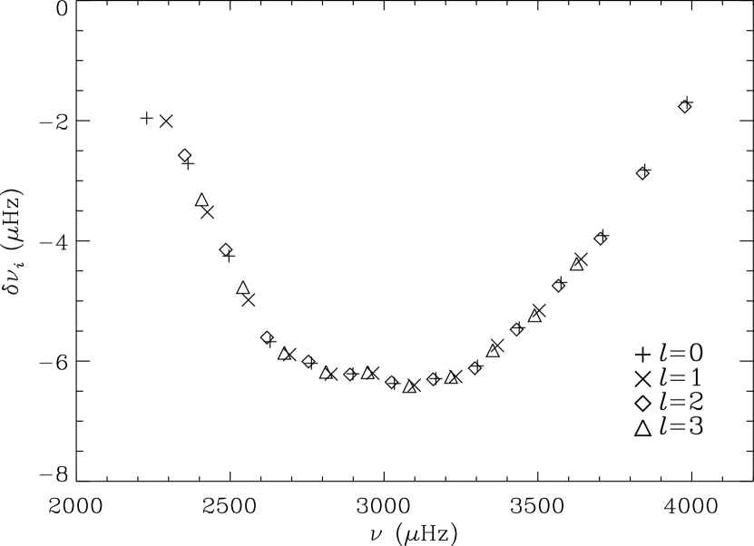
Figure 3: The symbols denote contributions $\delta\nu_{\boldsymbol{i}}$ to the frequencies $\nu_{\boldsymbol{i}}$ produced by the acoustic glitches of the Sun (see also Houdek & Gough, 2009b).

Following Houdek & Gough (2007b) we estimate the components of the displacement eigenfunction $\mn@boldsymbol{\xi}$ of a mode of oscillation of ${\cal M}_{\rm s}$, and the divergence, in separated form as products of spherical harmonics and functions of radius $r$, using the (hybrid) JWKB asymptotic approximation (e.g. Gough, 2007) for high order $n$:

$$\xi\simeq\left(\frac{K}{r^{2}\rho}\right)^{1/2}\cos\psi\,,\quad{\rm div}\mn@boldsymbol{\xi}\simeq\left(\frac{\pi\omega^{3}|x|}{\gamma_{1}pcr^{2}K}\right)^{1/2}{\rm Ai}(-x)\,,$$ (11)

where $\xi(r)$ is the $r$-dependent factor in the vertical component of $\mn@boldsymbol{\xi}$, having effective vertical wavenumber $K$, and $\omega=2\pi\nu$ is the angular frequency of oscillation; the argument $x$ of the Airy function Ai is given by

$$x:={\rm sgn}(\psi)\big{|}\frac{3}{2}\psi{\big{|}}^{2/3}$$ (12)

in terms of the phase $\psi(\tau)=\int K\,{\rm d}r$, which we approximate using a plane-parallel polytropic envelope of index $m$:

$$\mbox{$\psi(\tau)\simeq$}\left\{\begin{array}[]{lll}\mbox{$\kappa\omega\tilde{\tau}-(m+1)\cos^{-1}\left(\frac{m+1}{\omega\tilde{\tau}}\right)$}&\mbox{for $\tilde{\tau}>\tau_{\rm t}$}\,,\\ \\ \mbox{$|\kappa|\omega\tilde{\tau}-(m+1)\ln\left(\frac{m+1}{\omega\tilde{\tau}}+|\kappa|\right)$}&\mbox{for $\tilde{\tau}\leq\tau_{\rm t}$}\,,\end{array}\right.$$ (13)

in which $\tilde{\tau}=\tau+\omega^{-1}\epsilon$, with $\epsilon$ being a phase constant, and $\tau_{\rm t}$ is the associated acoustical depth of the upper turning point, at which the wavenumber $K$ vanishes. The function

$$\kappa(\tau)=\left[1-\left(\frac{m+1}{\omega\tilde{\tau}}\right)^{2}\right]^{1/2}\,$$ (14)

results from approximating $K$ as $c^{-1}(\omega^{2}-\omega^{2}_{\rm c})^{1/2}$ in which the acoustic cutoff frequency $\omega_{\rm c}$ is approximated by $(m+1)/\tilde{\tau}$. Following Houdek & Gough (2007b) we take $m=3.5$. The Airy function must be adopted in the expression for div$\mn@boldsymbol{\xi}$, which appears in the integral for $\delta_{\gamma}{\cal K}$ in equation (11), because the upper turning point of the highest-frequency modes is within the He I ionization zone where $\delta\gamma_{1}$ is nonzero. It is adequate to use the sinusoidal (JWKB) expression for both $\xi$ and the horizontal component of the displacement $\mn@boldsymbol{\xi}$ – which is determined as a horizontal derivative in div$\,\mn@boldsymbol{\xi}$ – in computing the inertia, given by equation (8), because almost all of the integral comes from regions far from the turning points. It is approximated by ${\cal I}\simeq\frac{1}{2}T\omega-\frac{1}{4}(m+1)\pi$ (Houdek & Gough, 2007b), where $T=\tau(0)$ is the acoustic radius of the star. The phase factor $\epsilon$ was introduced to take some account of the variation with $\omega$ of the location of the upper turning point.

Inserting these expressions into equations (7)–(9) yields the following approximation to the helium-glitch frequency component:

$$\delta_{\gamma}\nu = -\sqrt{2\pi}A_{\rm II}\Delta^{-1}_{\rm II}\left[\nu+\textstyle\frac{1}{2}(m+1)\nu_{0}\right]$$ (17)

$$\times\Bigl{[}\tilde{\mu}\tilde{\beta}\int_{0}^{T}\kappa^{-1}_{\rm I}{\rm e}^{-(\tau-\tilde{\eta}\tau_{\rm II})^{2}/2\tilde{\mu}^{2}\Delta^{2}_{\rm II}}|x|^{\frac{1}{2}}|{\rm Ai}(-x)|^{2}\,{\rm d}\tau$$

$$\;\;+\int_{0}^{T}\kappa^{-1}_{\rm II}{\rm e}^{-(\tau-\tau_{\rm II})^{2}/2\Delta^{2}_{\rm II}}|x|^{\frac{1}{2}}|{\rm Ai}(-x)|^{2}\,{\rm d}\tau\Bigr{]}\,,$$

where $\kappa_{i}:=\kappa(\tau_{i})$, and where we have introduced a frequency amplitude factor $A_{\rm II}=\frac{1}{2}\Gamma_{\rm II}T^{-1}$.

There are three additional components to $\Delta_{2}\nu_{i}$ that we must consider. The first is due to the abrupt variation in the vicinity of the base of the convection zone at $\tau_{\rm c}$. We model it with a discontinuity in $\omega^{2}_{\rm c}$ at $\tau_{\rm c}$ coupled with an exponential relaxation to the smooth model ${\cal M}_{\rm s}$ in the radiative zone beneath, with acoustical scale time $\tau_{0}{\color[rgb]{0,0,0}{=80{\rm s}}}$, as did Houdek & Gough (2007b). This leads to

$$\delta_{\rm c}\nu \simeq A_{\rm c}\nu_{0}^{3}\nu^{-2}\left(1+1/16\pi^{2}\tau_{0}^{2}\nu^{2}\right)^{-1/2}$$ (18)

$$\times \left\{\cos[2\psi_{\rm c}+\tan^{-1}(4\pi\tau_{0}\nu)]\!-\!(16\pi^{2}\tilde{\tau}_{\rm c}^{2}\nu^{2}\!+\!1)^{1/2}\right\}\,,$$ (19)

where $\psi_{\rm c}:=\psi(\tau_{\rm c})$ and $\tilde{\tau}_{\rm c}:=\tilde{\tau}(\tau_{\rm c})$, and $A_{\rm c}$ is proportional to the jump in $\omega^{2}_{\rm c}$.

The other two components, whose sum we denote by $\delta_{\rm u}\nu_{i}$, contain a part that is generated in the very outer layers of the star – by the ionization of hydrogen, the abrupt stratification of the upper superadiabatic boundary layer of the convection zone, and by nonadiabatic processes and Reynolds-stress perturbations associated with the oscillations, which are difficult to model (e.g. Rosenthal et al., 1995; Houdek, 2010) – and a part that results from the incomplete removal of the smooth component when taking a second difference. The latter was obtained from equation (2), and is given approximately by the second derivative of $\nu_{{\rm s}\boldsymbol{i}}$ with respect to $n$, regarded as a continuous variable, retaining only the leading term. The degree-dependent term is much smaller than the other, and it is adequate here to regard the entire contribution as part of the essentially degree-independent upper (near-surface) glitch term, even though it actually arises in part from refraction in the radiative interior. We approximate it as a series in inverse powers of $\nu$, truncated at the cubic order:

$$\Delta_{2}\delta_{\rm u}\nu_{\boldsymbol{i}}=\sum_{k=0}^{3}a_{k}\nu_{\boldsymbol{i}}^{-k}\,.$$ (20)

We appreciate that in principle there should be an additional contribution from the stellar atmosphere which, because it is produced far in the upper evanescent region of the mode, is a high power of $\nu$ (Christensen-Dalsgaard & Gough, 1980). However, for the Sun and Sun-like stars its contribution to the second differences, used for determining $\Gamma_{i}$, is small, as can be adduced from the work by Kjeldsen, Bedding & Christensen-Dalsgaard (2008). Its effect on the fitting of the smooth components $\nu_{{\rm s}{\boldsymbol{i}}}$ is mainly to distort the values of $B$, $E$ and $I$. However, these coefficients are not used for the $t_{\odot}$ and $Y_{0}(Z_{0})$ calibration. Accordingly, we can safely ignore this surface contribution. Doğan, Bonanno & Christensen-Dalsgaard (2011) have recently illustrated this general point with specific numerical examples.

The complete expression for the second difference

$$\Delta_{2{\boldsymbol{i}}}\nu\simeq\Delta_{2}(\delta_{\gamma}\nu_{\boldsymbol{i}}+\delta_{\rm c}\nu_{\boldsymbol{i}}+\delta_{\rm u}\nu_{\boldsymbol{i}})=:g_{\boldsymbol{i}}(\nu_{\boldsymbol{j}};\eta_{\alpha})$$ (21)

was then fitted to the second differences of the solar, or solar-model, frequencies to determine the coefficients $\eta_{\alpha}=(A_{\rm II}$, $\Delta_{\rm II}$, $\tau_{\rm II}$, $\epsilon_{\rm II}$, $A_{\rm c}$, $\tau_{\rm c}$, $\epsilon_{\rm c},a_{0},a_{1},a_{2},a_{3}),\,\alpha=1,...,11$. From the outcome, putative frequency contributions $\delta_{\rm u}\nu_{i}$ were obtained by summing the second differences (20) to yield

$$\delta_{{\rm u}}\nu_{\boldsymbol{i}} \simeq \tilde{A}+\tilde{B}\nu_{i}$$ (22)

$$\!\!+\!\! {\frac{1}{2}}\left[a_{0}\nu_{i}^{2}+2a_{1}\nu_{i}(\ln\nu_{\boldsymbol{i}}\!-\!1)-2a_{2}\ln\nu_{\boldsymbol{i}}+a_{3}\nu_{i}^{-1}\right]$$ (24)

$$\times(\nu_{n+1,0}-\nu_{n-1,0})$$

$$\equiv \tilde{A}+\tilde{B}\nu_{\boldsymbol{i}}+F_{{\rm u}{\boldsymbol{i}}}\,.$$ (25)

The initially arbitrary constants of summation $\tilde{A}$ and $\tilde{B}$ were selected in such a way as to minimize the $L_{2}$ norm of $\delta_{\rm u}\nu_{\boldsymbol{i}}$, namely $\sum_{\boldsymbol{i}}(\tilde{A}+\tilde{B}\nu_{\boldsymbol{i}}+F_{{\rm u}{\boldsymbol{i}}})^{2}$, as did Houdek & Gough (2009a).

The fitting of the second-differences was accomplished by minimizing

$$E_{\rm g}=(\Delta_{2{\boldsymbol{i}}}\nu-g_{\boldsymbol{i}}){\rm C}^{-1}_{\Delta{\boldsymbol{ij}}}(\Delta_{2{\boldsymbol{j}}}\nu-g_{\boldsymbol{j}})$$ (26)

using the value of $\nu_{0}$ obtained from the fitting of expression (2). (That fitting was accomplished by minimizing the appropriately weighted mean-square difference $E_{\rm s}$ – defined in § 2.4 – from the smooth frequencies $\nu_{{\rm s}{\boldsymbol{i}}}$, which are themselves derived from the raw frequencies by subtracting the glitch contribution obtained by minimizing $E_{\rm g}$; the two minimizations were carried out iteratively in tandem.) Here C${}^{-1}_{\Delta{\boldsymbol{ij}}}$ is the $({\boldsymbol{i}},{\boldsymbol{j}})$ element of the inverse of the covariance matrix C_Δ of the observational errors in $\Delta_{2{\boldsymbol{i}}}\nu$, computed, perforce, under the assumption that the errors in the frequency data $\nu_{\boldsymbol{i}}$ are independent. The resulting covariance matrix C_ηαγ of the errors in $\eta_{\alpha}$ was established by Monte Carlo simulation, using 6000 realizations of Gaussian-distributed errors in the raw data with variance in accord with the published standard errors. In carrying out the simulations we omitted the surface term $\delta_{\rm u}\nu_{\boldsymbol{i}}$, which has insignificant influence on the statistics.

Figure 4: Denotation of the eleven solar models which we have used for calculating the partial derivatives $H_{\alpha\beta}$, calibrated to a present radius ${\rm R}_{\odot}=6.9599\times 10^{10}$ cm and luminosity ${\rm L}_{\odot}=3.846\times 10^{33}$erg s^-1. The ‘central model’ is Model 0; the sequence of the five models (0-4) has a constant value of $Z_{0}=0.02$ but varying age $t_{\star}$ (4.15, 4.37, 4.60, 4.84, 5.10) Gy; the second sequence, of seven models (0,5-10), has constant age $t_{\star}=4.60\,$Gy but varying $Z_{0}$ (from 0.016 to 0.022 in uniform steps of 0.001).

The outcome of the fitting to the BiSON data is displayed in Fig. 2: the upper panel displays the second differences, together with the complete fitted formula (21) (solid curve) and its individual smooth frequency contribution $\delta_{\rm u}\nu_{i}$ estimated by equation (20); the corresponding oscillatory frequency contributions $\Delta_{2}\delta_{\gamma}\nu$ (dotted and solid curves for the two stages of helium ionization) and $\Delta_{2}\delta_{\rm c}\nu$ (dot-dashed curve) are illustrated in the lower panels of Fig. 2. All the frequencies displayed in the figure have been used in equation (26) for fitting expression (21).

In Fig. 3 is displayed the sum of all acoustic glitch contributions to the frequencies estimated by fitting equation (21) to the low-degree solar frequencies observed by BiSON (Basu et al., 2007).

Figure 5: Integrand $-({\rm d}c/{\rm d}x)/x$ of $A$ as a function of radius fraction $x:=r/R$ for the calibrated solar models 5, 0 and 10 with varying $Z_{0}$ at constant age $t_{\odot}=4.60\,$Gy. The dashed, solid and dot-dashed curves are the results for models 5 ($Z_{0}$=0.016), 0 ($Z_{0}=0.020$) and 10 ($Z_{0}$=0.022) respectively. Note that the sensitivity to $Z_{0}$ lies mainly near the centre; the same is so for the sensitivity to $t_{\star}$ (Gough & Novotny, 1990).

2.4 Calibration for age and chemical composition

We subtract the glitch contributions $\delta\nu_{\boldsymbol{i}}$ from the full frequencies to obtain corresponding glitch-free frequencies $\nu_{{\rm s}{\boldsymbol{i}}}$. The procedure is carried out for the solar observations, for the eigenfrequencies of the reference solar model, and for the grid of models used for evaluating derivatives of the fitting parameters with respect to $t_{\star}$ and $Z_{0}$ (see Fig. 4). Then we iterate the parameters defining the reference model by minimizing $E_{\rm s}:=(\nu_{{\rm s}{\boldsymbol{i}}}-S_{\boldsymbol{i}}){\rm C}^{-1}_{{\rm s}{\boldsymbol{ij}}}(\nu_{{\rm s}{\boldsymbol{j}}}-S_{\boldsymbol{j}})$, where C_s is the covariance matrix of the statistical errors in $\nu_{{\rm s}{\boldsymbol{i}}}$, which are determined from the independent observational errors in $\nu_{\boldsymbol{i}}$ and the covariance matrix C${}_{\eta_{\alpha\beta}}$, to obtain both the coefficients $\xi_{\beta}$ and the covariance matrix C_ξβδ of their errors. In this iteration process for $\xi_{\beta}$, only glitch-free frequencies $\nu_{{\rm s}{\boldsymbol{i}}}$ with $k=n+\frac{1}{2}l\geq 15$ were considered, because the asymptotic expression (2) is not sufficiently accurate for lower values of $k$. Each component of $\xi_{\beta}$ is an integral of a function of the equilibrium stratification. Some of these are displayed in Fig. 1. The integrals $A,C$ and $F$ are those of particular importance to our analysis, because $C$ and $F$ are dominated by conditions in the core, and, although the contributions to $A$ from the core and the rest of the star are roughly equal in magnitude (and potentially have opposite signs), the contribution from the envelope is relatively insensitive to $t_{\star}$ (Gough & Novotny, 1990) and $Z_{0}$ (Fig. 5). The integrands in the remaining integrals are either more evenly distributed throughout the Sun or are concentrated near the surface.

The differences between the smoothed frequencies $\nu_{{\rm s}{\boldsymbol{i}}}$ and the fitted asymptotic expression $S_{\boldsymbol{i}}$ given by equation (2) are displayed in Fig. 6 for the BiSON data (left panel) and for the central model m0 (right panel).

Figure 6: Differences between smoothed frequencies $\nu_{{\rm s}{\boldsymbol{i}}}$, of the Sun (left) and central Model 0 (right), and the correspondingly fitted asymptotic expression $S_{\boldsymbol{i}}$ given by (2). Modes of like degree $l$ are connected by solid lines. Contrary to the opinions of some commentators, the curves are not like the oscillatory contribution from $\delta\gamma_{1}/\gamma_{1}$, for rather than decreasing, the amplitude of the undulation increases with increasing $\nu$ (cf. Fig. 2), indicating discrepancies in the very outer layers.

We have carried out age calibrations using various combinations of the parameters

$$\zeta_{\alpha}=(\hat{A},\hat{C},\hat{F},-\delta\gamma_{1}/\gamma_{1}),\qquad\alpha=1,...,4\,,$$ (27)

where $-\delta\gamma_{1}/\gamma_{1}=A_{\rm II}/\sqrt{2\pi}\nu_{0}\Delta_{\rm II}$ is a measure of the maximum depression in $\gamma_{1}$ in the second helium ionization zone, and which for convenience we sometimes denote by $\hat{\Gamma}$. The values of $-\delta\gamma_{1}/\gamma_{1}$ and the asymptotic coefficients $A,C,F$ appearing in expression (2), determined from the observed seismic frequencies, are listed in Table 1 for the Sun, and are plotted in Fig. 7 for the eleven calibrated grid models. Presuming, as is normal, that the reference model is parametrically close to the Sun, we first carry out a single iteration by approximating the reference value $\zeta^{\rm r}_{\alpha}$ by a two-term Taylor expansion about the value $\zeta^{\odot}_{\alpha}$ of the Sun:

$$\zeta^{\rm r}_{\alpha}=\zeta^{\odot}_{\alpha}-\left(\frac{\partial\zeta_{\alpha}}{\partial t_{\star}}\right)_{\!\!Z_{0}}\Delta\,t_{\star}-\left(\frac{\partial\zeta_{\alpha}}{\partial Z_{0}}\right)_{\!\!t_{\star}}\Delta Z_{0}+\epsilon_{\zeta\alpha}\,,$$ (28)

where $\Delta\,t_{\star}$ and $\Delta Z_{0}$ are the deviations of the age $t_{\odot}$ and initial heavy-element abundance $Z_{0}$ of the Sun from the corresponding values of the reference model; $\epsilon_{\zeta\alpha}$ are the formal errors in the calibration parameters, whose covariance matrix C_ζαβ can be derived from C_ξβδ and C_ηαγ. A (parametrically local) maximum-likelihood fit then leads to the following set of linear equations:

$$H_{\alpha j}{\rm C}^{-1}_{\zeta\alpha\beta}H_{\beta k}\Theta_{0k}=H_{\alpha j}{\rm C}^{-1}_{\zeta\alpha\beta}\Delta_{0\beta}\,,$$ (29)

in which $\Theta_{k}=(\Delta t_{\star},\Delta Z)+\epsilon_{\Theta k}=\Theta_{0k}+\epsilon_{\Theta k}$, $k=1,2$, is the solution vector subject to (correlated) errors $\epsilon_{\Theta k}$, and $\Delta_{\beta}=\zeta^{\star}_{\beta}-\zeta^{\rm r}_{\beta}+\epsilon_{\zeta\beta}=\Delta_{0\beta}+\epsilon_{\zeta\beta}$; the partial derivatives are denoted by $H_{\alpha j}=[(\partial\zeta_{\alpha}/\partial t_{\star})_{Z_{0}},(\partial\zeta_{\alpha}/\partial Z)_{t_{\star}}]$, $j=1,2$.

A similar set of equations is obtained for the formal errors $\epsilon_{\Theta k}$:

$$H_{\alpha j}{\rm C}^{-1}_{\zeta\alpha\beta}H_{\beta k}\epsilon_{\Theta k}=H_{\alpha j}{\rm C}^{-1}_{\zeta\alpha\beta}\epsilon_{\zeta\beta}\,,$$ (30)

from whose solution the error covariance matrix C${}_{\Theta kq}=\overline{\epsilon_{\Theta k}\epsilon_{\Theta q}}$ can be computed.

Table 1: Asymptotic coefficients for the Sun obtained from (linear) fitting to the glitch-free (smoothed) BiSON frequencies $\nu_{\rm s}$ the expression (2) by weighted least squares $E_{\rm s}$.

$\nu_{0}$ ($\mu$Hz)	$A$	$C$	$F$	$-\delta\gamma_{1}/\gamma_{1}$
136.71	0.3005	1.912	69.83	0.04538

The partial derivatives $H_{\alpha j}$ were obtained from the set of eleven calibrated evolutionary models (see Fig. 4) of the Sun that were used in a similar calibration by Houdek & Gough (2007a). The models were computed with the evolutionary programme by Christensen-Dalsgaard (2008), adopting the Livermore equation of state and the OPAL92 opacities. The set comprises two sequences: one has a constant value of the heavy-element abundance $Z_{0}=0.020$ but varying age ($t_{\star}=4.15,...,5.10\,$Gy in uniform steps of 0.05 in $\ln t_{\star}$); the other has constant age $t_{\star}=4.60\,$Gy but varying $Z_{0}$ ($Z_{0}$=0.016,…,0.022 in uniform steps of 0.001). Note that, for prescribed relative abundances of heavy elements, the condition that the luminosity and radius of the Sun agree with observation defines a functional relation between $Y_{0},Z_{0}$ and $t_{\star}$ amongst the models. In Fig. 7 are plotted the seismic parameters $A,C,F$ and $-\delta\gamma_{1}/\gamma_{1}$ of the eleven models, each calibrated to the solar radius and luminosity, for determining the partial derivatives $H_{\alpha j}$ of $A,C,F$ and $-\delta\gamma_{1}/\gamma_{1}$ with respect to stellar age $t_{\star}$ and initial heavy-element abundance $Z_{0}$. The values of the partial (logarithmic) derivatives $H_{\alpha j}$ so obtained are listed in Table 2. Notice that within the range of model parameters that we have considered, the derivatives are almost constant.

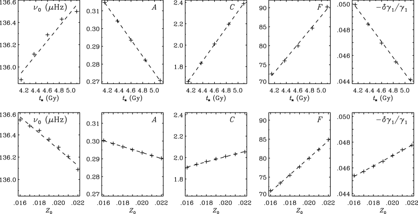
Figure 7: Seismic parameters $\nu_{0},A,C,F$ and $-\delta\gamma_{1}/\gamma_{1}$ of eleven calibrated solar models from which their partial derivatives $H_{\alpha j}$ with respect to stellar age $t_{\star}$ and initial heavy-element abundance $Z_{0}$, listed in Table 2, are obtained.

Table 2: Partial logarithmic derivatives ($H_{\alpha j}$) obtained from the two sets of calibrated evolutionary models for the Sun denotated in Fig. 4. They were determined by linear regression about the central Model 0.

$\left(\frac{\partial\ln\nu_{0}}{\partial\ln t_{\star}}\right)_{Z_{0}}$	$\left(\frac{\partial\ln\nu_{0}}{\partial\ln Z_{0}}\right)_{t_{\star}}$	$\left(\frac{\partial\ln A}{\partial\ln t_{\star}}\right)_{Z_{0}}$	$\left(\frac{\partial\ln A}{\partial\ln Z_{0}}\right)_{t_{\star}}$	$\left(\frac{\partial\ln C}{\partial\ln t_{\star}}\right)_{Z_{0}}$	$\left(\frac{\partial\ln C}{\partial\ln Z_{0}}\right)_{t_{\star}}$
0.0220	-0.00997	-0.733	-0.107	1.771	0.231
$\left(\frac{\partial\ln F}{\partial\ln t_{\star}}\right)_{Z_{0}}$	$\left(\frac{\partial\ln F}{\partial\ln Z_{0}}\right)_{t_{\star}}$	$\left(\frac{\partial\ln(-\delta\gamma_{1}/\gamma_{1})}{\partial\ln t_{\star}}\right)_{Z_{0}}$	$\left(\frac{\partial\ln(-\delta\gamma_{1}/\gamma_{1})}{\partial\ln Z_{0}}\right)_{t_{\star}}$	$\left(\frac{\partial\ln Y_{0}}{\partial\ln t_{\star}}\right)_{Z_{0}}$	$\left(\frac{\partial\ln Y_{0}}{\partial\ln Z_{0}}\right)_{t_{\star}}$
1.057	0.539	-0.607	0.163	-0.173	0.334

3 Results

Provided that the reference model is close to the Sun, the single iteration described in the previous section should provide as reliable an estimate of ($\Delta t_{\odot},\;\Delta Z_{0}$) as the calibration is currently able to provide. We therefore discuss at first the results of single iterations. Calibrations were carried out using different combinations of the parameters $\zeta_{\alpha}$ and two different reference models. They are summarized in Table 3. The older reference model is the central ‘Model 0’ which has age $t_{\star}=4.600\,$Gy; the second is ‘Model 2’, which has an age $t_{\star}=4.370\,$Gy. Because the acoustic properties of the stars in the grid vary almost linearly with $t_{\star}$ and $Z_{0}$ the error covariance matrices associated with the single iteration are indistinguishable. We adopted the same physics as in Model S (Christensen-Dalsgaard et al., 1996) in the evolutionary calculations of both models. We notice by comparing rows 4 and 6 with rows 5 and 7 in Table 3 that calibrations without $\delta\gamma_{1}/\gamma_{1}$ are less stable to a change in the reference model than are the calibrations including $\delta\gamma_{1}/\gamma_{1}$. They are possibly less reliable, for the reasons explained in the introduction, although the result may perhaps be simply a symptom of slower convergence.

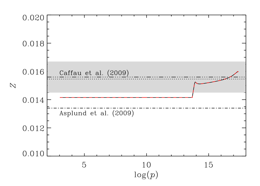
Figure 11: Heavy-element abundance $Z$ as a function of the depth-coordinate $\log(p)$ obtained from the reference Models 0 ($t_{\star}=4.60\,$Gy, solid black curve) and 2 ($t_{\star}=4.37\,$Gy, dashed red curve) after five calibration iterations. Results from spectroscopic analyses based on numerical simulations by Asplund et al. (2009) (dot-dashed line) and Caffau et al. (2009) (triple-dot-dashed line) of the convectively driven macroscopic motion in the atmosphere are indicated; the shaded area indicates the reported error bars by Caffau et al. (2009). The initial (zero age) value $Z_{0}$ of both reference models is indicated by the dotted line. After five calibration iterations both reference models have a surface heavy-element abundance $Z_{\rm s}=0.0142$; the age obtained from the 4.60 Gy reference model (Model 0) is 4.604$\pm 0.039\,$Gy, and that from the 4.37 Gy reference model (Model 2) is 4.603$\pm 0.039\,$Gy (see also Table 5).

To ascertain whether the entire calibration procedure converges, we have performed several additional iterations. At each iteration the corrections $\Delta t_{\star}$ and $\Delta Z_{0}$ are used to define parameters of a new reference model, which is then constructed by performing another evolutionary calculation, followed by the evaluation of a new set of corrections $\Delta t_{\star}$ and $\Delta Z_{0}$ as before. We repeated this for five iterations, for each of the two reference models, obtaining the two ‘final’ reference models, listed in Table 5, for two different combinations of $\zeta_{\alpha}$, whose present heavy-element abundance $Z$ is displayed in Fig. 11. The progressive corrections $\Delta t_{\star}$ and $\Delta Z_{0}$ are plotted in Fig. 8. In carrying out the iterations we did not recompute the partial derivatives $H_{\alpha j}$ and the corresponding error covariance matrices. To have done so would have been computationally much more expensive, would have been likely not to have speeded up convergence by very much, and would not have altered the final solution. The final residuals $\Delta_{\rm s}:=\nu_{{\rm s}{\boldsymbol{i}}}-S_{\boldsymbol{i}}$ are barely distinguishable from those from the Sun, as illustrated in Fig. 9.

Table 3: Age calibrations with different combinations of $\zeta_{\alpha}$ and for the two reference models: Model 0 with an age $t_{\star}=4.60\,$Gy and Model 2 with an age $t_{\star}=4.37\,$Gy, both computed with an initial heavy-element abundance $Z_{0}\,=\,0.02$ adopting the Grevesse & Noels (1993) solar composition. The first three columns show the results adopting Model 0 as the reference model, the fourth, fifth and sixth columns display the results for Model 2. The remaining three columns are the values of the error covariance matrix C_Θ for both reference models.

$\zeta_{\alpha}$	$t_{\odot}$ (Gy)	$Z_{0}$	$Y_{0}$	$t_{\odot}$ (Gy)	$Z_{0}$	$Y_{0}$	C${}^{1/2}_{\Theta 11}$	$-(-{\rm C}_{\Theta 12})^{1/2}$	C${}^{1/2}_{\Theta 22}$
$\hat{A},\hat{C},\hat{F},-\delta\gamma_{1}/\gamma_{1}$	4.592	0.0156	0.252	4.597	0.0155	0.251	0.039	0.0013	0.0005
$\hat{A},\hat{F},-\delta\gamma_{1}/\gamma_{1}$	4.580	0.0157	0.252	4.582	0.0156	0.251	0.045	0.0016	0.0006
$\hat{C},\hat{F},-\delta\gamma_{1}/\gamma_{1}$	4.591	0.0157	0.252	4.595	0.0155	0.251	0.044	0.0004	0.0005
$\hat{A},\hat{C},-\delta\gamma_{1}/\gamma_{1}$	4.597	0.0160	0.254	4.603	0.0160	0.253	0.045	0.0036	0.0008
$\hat{A},\hat{C},\hat{F}$	4.619	0.0153	0.252	4.632	0.0151	0.248	0.095	0.0104	0.0013
$\hat{A},\hat{C}$	4.638	0.0147	0.246	4.654	0.0143	0.245	1.049	0.1791	0.0306
$\hat{A},-\delta\gamma_{1}/\gamma_{1}$	4.588	0.0159	0.253	4.592	0.0158	0.253	0.149	0.0222	0.0039

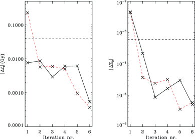
Figure 8: Corrections of the solar age $t_{\odot}$ (left panel) and initial heavy-element abundance $Z_{0}$ (right panel) for six calibration iterations and the combination $\hat{A},\hat{C},\hat{F}$ and $-\delta\gamma/\gamma$ for two reference models with an initial age of $t=4.60\,$ (solid black curves) and $t=4.37\,$Gy (dashed red curves) and initial heavy-element abundance $Z_{0}=0.02$. The horizontal dashed lines are the estimated 1$\,\sigma$ error bars of the calibrated age and initial heavy-element abundance.

Error contours corresponding to the calibration from Model 0 in the first row of Table 5 are plotted in Fig. 10. Corresponding contours for Model 2 are the same, except that their centres are displaced to (4.603 Gy, 0.0155). One can adduce from our description of the analysis in § 2.4 that our current treatment of the errors is not completely unbiassed, because, aside from $\nu_{0}$, we assess the error covariances of the parameters defining the smooth and the glitch components independently; however, the potential bias is of the order of only $|\delta\nu_{i}/\nu_{i}|$ or less, which is small.

Fig. 11 depicts the heavy-element profiles after five iterations from the two reference models (Models 0 and 2). Both models have a surface value $Z_{\rm s}=0.0142\pm 0.0005$, which is about 6% higher than the value of $Z_{\rm s}=$0.0134 reported by Asplund et al. (2009) and about 9% smaller than the value of $Z_{\rm s}=0.0156\pm 0.0011$ reported by Caffau et al. (2009). The error-bars of Caffau’s $Z_{\rm s}$ value, obtained from numerical simulations, is indicated by the shaded region.

The calibrated age inferred from Model 0 after five iterations is 4.604$\pm 0.039\,$Gy, and that from Model 2 is 4.603$\pm 0.039\,$Gy, using the parameter combination $\hat{A},\hat{C},\hat{F}$ and $-\delta\gamma_{1}/\gamma_{1}$. The corresponding calibrations from Models 0 and 2 for the combination $\hat{C},\hat{F}$ and $-\delta\gamma_{1}/\gamma_{1}$ are $4.602\pm 0.044\,$Gy and $4.601\pm 0.044\,$Gy, respectively. Table 5 summarizes the calibrations after five iterations from reference Models 0 and 2.

Figure 9: Differences between residuals $\Delta_{\rm s}:=\nu_{{\rm s}\boldsymbol{i}}-S_{\boldsymbol{i}}$ obtained from the frequencies of the Sun, $\Delta_{{\rm s},\odot}$, and the calibrated model after five iterations from reference Model 0, $\Delta_{{\rm s,m}}$, where expression $S_{\boldsymbol{i}}$ given by Eq. (2) was fitted to the smoothed frequencies $\nu_{{\rm s}\boldsymbol{i}}$.

4 Discussion

In attempting to estimate the main-sequence age of the Sun it is prudent to adopt diagnostic quantities that are insensitive to properties that one believes not to be directly pertinent. As the Sun evolves on the main sequence it converts hydrogen into helium in the core. According to theoretical models it liberates energy at a rate whose dependence on time, measured in units of the age $t_{\star}$, is not very sensitive to uncertain parameters defining those models, such as the initial heavy-element abundance $Z_{0}$, provided that the models have been calibrated to reproduce the luminosity and radius observed today (cf. Gough, 1990b). The same is true of the quantity of hydrogen consumed, mainly because the nuclear relations are dominated by a single branch of the pp chain, namely ppI, for which there is a tight link between fuel consumption and thermal energy release. Therefore one would expect there to be a robust link between main-sequence age and the total amount of hydrogen consumed: the integral $\Delta H:=\int h(r)\rho r^{2}\,{\rm d}r:=4\pi\int\left[X_{0}-X(r)\right]\rho r^{2}\,{\rm d}r$ should be a good indicator of the age $t_{\odot}$. It can be calibrated using seismic diagnoses of the mean molecular mass $\mu(r)$ provided that processes other than nuclear reactions that can change $X(r)$, such as gravitational settling and diffusion, are taken adequately into account.

In perhaps its simplest form, solar evolution involves computing models of constant mass in hydrostatic equilibrium. The models usually depend on three initial parameters: the initial abundances of, say, helium, $Y_{0}$, and the heavy elements, $Z_{0}$, and a mixing-length parameter $\alpha_{\rm c}$ which is normally held constant. It is usual to fix the relative abundances of all elements other than hydrogen and helium, a procedure which we too have adopted here. Demanding that the luminosity and radius of the model agree with present-day observation relates two of those parameters, say $\alpha_{\rm c}$ and $Y_{0}$, to the third, $Z_{0}$, for any $t_{\star}$. Thus one obtains a two-parameter set of potentially acceptable models, which here we characterize by the values of $t_{\star}$ and $Z_{0}$, and which we attempt to calibrate with helioseismic data.

Several diagnostics have been used in the past. As mentioned in the introduction, the first to be used for a full calibration were the two mean small separations $d_{0}$ and $d_{1}$ (Gough, 2001), averages over $n$ of $d_{n,0}$ and $d_{n,1}$, the hope being that the differences in the way in which the two quantities sample the core would be adequate to disentangle $t_{\odot}$ and $Z_{0}$. Unfortunately, given the precision of the data at the time, that could not be accomplished to a useful precision. Moreover, by inspecting the dependence of the calibration on the range of frequencies over which the averages $d_{0}$ and $d_{1}$ were determined, there was evidence of contamination by an oscillatory component to the signatures from seismically abrupt variations of the stratification in and at the base of the convection zone. This component is particularly visible in second- and higher-order frequency differences with respect to $n$ (e.g. Gough, 1990a; Ballot, Turck-Chièze & García, 2004; Basu & Mandel, 2004).

There were several obvious improvements to the original calibration based solely on fitting to raw frequencies a smooth-asymptotic formula, such as equation (2) or derivatives of it, that were required to be put into place in order to obtain a more reliable calibration. The first that we have made is to isolate much of the signal from the abrupt variation of the thermodynamic properties in the convection zone. The intention was two-fold: First, by removing the oscillatory component from the stratification one is left with a smooth model for which the simple asymptotic expression (2) is more nearly valid; second, its amplitude provides an independent measure of the helium abundance $Y_{\rm s}$ in the convection zone (Houdek & Gough, 2007b) through the magnitude of the depression in $\gamma_{1}$ in the ionization zones. The latter provides, via stellar-evolution theory, the value of $Y_{0}$ – and therefore $X_{0}(Z_{0})$ – in the core, which is required for determining the hydrogen deficit $h(r)$. In carrying out the analysis, the variation in $\gamma_{1}$ has been represented by two Gaussian functions of acoustic depth, as recommended by Gough (2002) and Houdek & Gough (2004), which has been found to reproduce the oscillation frequencies more faithfully than either the simple discontinuity that was adopted by Basu et al. (2004), Basu & Mandel (2004) and Mazumdar & Michel (2010), and the triangular form adopted by Monteiro & Thompson (1998, 2005) and Verner, Chaplin & Elsworth (2006); presumed discontinuities in $\gamma_{1}$ or its derivatives cause the amplitude of the predicted oscillatory feature to decay too slowly with frequency (Houdek & Gough, 2004), which, although apparently not very deleterious for the Sun, may be a serious deficiency for other stars.

Figure 10: Error ellipses for the calibration using the combination $\hat{A},\hat{C},\hat{F}$, $-\delta\gamma_{1}/\gamma_{1}$ and Model 0 as the reference model: solutions $(t_{\odot},Z_{0})$ satisfying the frequency data within 1, 2 and 3 standard errors in those data reside in the inner, intermediate and outer ellipses, respectively.

Another improvement is to remove from the diagnostics more of the influence of regions of the Sun that are outside the core. The absolute frequency of a low-degree mode of oscillation feels almost all of the interior structure of the star in inverse proportion to the sound speed along a ray path, except near the surface where the influence of the rapid variation of the acoustical cutoff frequency $\omega_{\rm c}$ dominates. The latter is largely eliminated in the small frequency separation, because the eigenfunctions in the very surface layers are almost independent of $L$, and therefore subtracting two modes of nearly the same frequency entails a high level of cancellation. However, the cancellation is not complete, simply because the frequencies of the two modes are not exactly the same. As Ulrich (1986) has pointed out, the ratio $R_{l}$ of the small separation $d_{l}$ to the large separation $\Delta_{l}$ is a more direct measure of age, for it isolates more effectively the nonhomologous aspects of the evolution (Gough, 1990b), and it more effectively eliminates the influence of the outermost layers of the Sun, as can easily be appreciated by comparing the formulae for $d_{l}$ and $R_{l}$ implied by the asymptotic expression (2). Roxburgh & Vorontsov (2003) and Otí Floranes, Christensen-Dalsgaard & Thompson (2005) have advocated that it be used for core calibration instead of $d_{l}$, and recently Doğan, Bonanno & Christensen-Dalsgaard (2011) have illustrated its robustness numerically. Here we have gone further by adopting as diagnostics the factors $\hat{A}$, $\hat{C}$, and $\hat{F}$, integrals of the solar structure which sense variations in conditions even more concentrated towards the centre of the star.

One could consider going even further by trying to replace the set of diagnostic factors with a single combination of $\hat{A}$, $\hat{C}$ and $\hat{F}$ designed to eliminate the influence of the surface layers as much as possible, analogous to the procedure adopted by Gough & Kosovichev (1988) and Kosovichev et al. (1992); that is tantamount to using a judiciously selected combination of small separation ratios $R_{l}$. Because $\hat{A}$, $\hat{C}$ and $\hat{F}$ depend differently on the core stratification, the simultaneous use of all three quantities provides some information about the manner in which $X$ varies with $r$. It is therefore to be hoped that the calibration is more secure than one using just $d_{l}$ or $R_{l}$. It is worth mentioning at this juncture that the integrand for $\hat{A}$ is not actually negligible outside the core, as can be seen from Fig. 1; indeed it has been known for some time that the integrand continues to the surface with approximately the same magnitude as it has at $r/R=0.5$ (Gough, 1986b, see also Fig. 5), and that the integral is dominated by conditions outside the core. However, it appears that only the inner parts change as $t_{\star}$ and $Z_{0}$ vary, and therefore that $\hat{A}$ is at least a fairly good diagnostic for our purposes. We note, however, that there is some contamination from outside the core, as is hinted in Table 3 in which it is recorded that $|C_{\Theta 12}|$ is smallest when $\hat{A}$ is not used in the calibration.

It is also important to include the diagnostic $\hat{\Gamma}:=-\delta\gamma_{1}/\gamma_{1}$, which measures the helium abundance $Y_{\rm s}$ in the convection zone, for that reflects a rather different aspect of the core structure and thereby enables a much more precise determination of $t_{\odot}$ and $Z_{0}$, as evinced by Table 3, and which was already evident in an earlier phase of the investigation (Houdek & Gough, 2007a). Whether or not the outcome is more accurate depends on the reliability of the procedure to account for gravitational settling, which relates $Y_{\rm s}$ in the surface to the value of $Y_{0}$ which controls conditions in the core. It should be pointed out also that $\hat{\Gamma}$ is not an uncontaminated measure of $Y_{\rm s}$, because it depends also on the entropy in the deep adiabatically stratified convection zone (Houdek & Gough, 2007b), and perhaps in reality also on the existence of an intense magnetic field (see below). Our procedure could be made more reliable if we could find an alternative diagnostic that senses $Y_{\rm s}$ more directly.

Further remarks about the influence of the outer layers, or the elimination thereof, are in order: In fitting the resolvable glitch contribution to the data an approximation to the unresolvable contribution from hydrogen ionization and the upper superadiabatically stratified boundary layer was included, equivalent to a cubic form in $\nu^{-1}$ added to the second differences (Houdek & Gough, 2007b). Associated with the resolvable glitches are smooth contributions which were ignored in the initial calibration for $t_{\odot}$ and $Z_{0}$ (Houdek & Gough, 2007a). Subsequently they were taken explicitly into account, thereby removing a bias in the procedure (Houdek & Gough, 2009a, b) and, it is to be supposed, improving the accuracy of the calibration. It should be mentioned, however, that we have not taken explicit account of putative errors in our modelling of the outermost layers of the Sun. Christensen-Dalsgaard & Gough (1980) found that were the oscillations to be adiabatic, the effect of the atmosphere would be to add to the frequencies a term $\delta$ that is itself a rapid function of frequency: $\delta\propto\nu^{b}$ with $b=2(m+1)$ for $\nu/\nu_{\rm c}\ll 1$, where $\nu_{\rm c}$ is the cyclic cutoff frequency $\omega_{\rm c}/2\pi$ and $m$ is an effective polytropic index in the vicinity of the upper turning point, which, from fitting a (smooth) asymptotic frequency formula to solar data, is expected to have a value of about 3 (Gough, 1986a; Houdek & Gough, 2007b); furthermore ${\rm d}\ln\delta/{\rm d}\ln\nu$ decreases with increasing $\nu$ as $\nu/\nu_{\rm c}$ approaches and exceeds unity. Kjeldsen, Bedding & Christensen-Dalsgaard (2008) found that in the Sun $b$ decreases to about 4.9 for $\nu\simeq 3\,$mHz, which is not entirely inconsistent with this finding.

We note, furthermore, that the influence of the perturbations on the Reynolds stress induced by the oscillations also has a component that increases with $\nu$, but more slowly than the effect of a perturbation in the atmosphere (e.g. Gough, 1986b; Balmforth, 1992; Rosenthal et al., 1995; Houdek, 2010). This result may also be partially responsible for the exponent $b$ being somewhat less than the expected value of 2$(m+1)$. Doğan, Bonanno & Christensen-Dalsgaard (2011) found that taking the correction into account obviates the necessity to use $R_{l}$ instead of $d_{l}$ in a simple model calibration for $t_{\odot}$ in which $Z_{0}$ is held fixed, and yields results similar to those obtained from $R_{l}$ with no surface term. This suggests that our neglect of the near-surface adjustment – a device which we adopted to maintain a workable number of unknown parameters in the fitting – may not be severely deleterious. Nonetheless, the approximation deserves further scrutiny.

We have also been somewhat cavalier in our modelling of the acoustic glitches at the base of the convection zone. In particular, we have modelled them as a simple discontinuity in the second derivative of the density together with an exponential recovery beneath (Houdek & Gough, 2007b) to represent standard solar models. Again, we have taken this approach for our convenience; after all, the sole purpose of modelling the glitch was to remove it. However, we are aware that we have not adequately taken account of the stratification of the tachocline, and that by so doing we risk not having eliminated adequately its contribution to the frequencies, and thereby may have biassed our final result. Indeed, it is evident that we have not been able to fit for the rapidly oscillating component of the second differences to the solar data as well as we have to the frequencies of a standard solar model, suggesting that there might be room for further improvement of the theory. Monteiro & Thompson (2005) and Christensen-Dalsgaard et al. (2011) have gone some way in making such improvements, with the intention of studying the stratification at the base of the convection zone itself. It behoves us to do so too. In this regard we observe that the differences between the residuals from the Sun and the calibrated model, displayed in Fig. 9, show evidence of undersampled high-frequency oscillations that are $l$ dependent, hinting that the tachocline structure might be aspherical.

Table 4: Age calibrations for fixed initial heavy-element abundance $Z_{0}=0.019628$ (the value adopted for Model S; Christensen-Dalsgaard et al. 1996) and $Z_{0}=0.014864$ (the value adopted for a solar model assuming the Asplund et al. 2009 abundances; see also Christensen-Dalsgaard & Houdek 2010). Results are shown for the combinations $\zeta_{\alpha}=(\hat{A},\hat{C},\hat{F})$, $(\hat{A},\hat{C})$ and $(\hat{A})$, and for two reference models: Model 0 with an age $t_{\star}=4.60\,$Gy and Model 2 with an age $t_{\star}=4.37\,$Gy. The first three columns show the calibrated ages and associated errors $\epsilon_{\Theta}$ for both reference models computed with constant $Z_{0}=0.019628$; the last three columns show the results for the age calibration of both reference models computed with constant $Z_{0}=0.014864$. For the $Z_{0}=0.019628$ age calibration the reference models and derivatives $H_{\alpha}=({\rm d}\hat{A}/{\rm d}t,{\rm d}\hat{C}/{\rm d}t,{\rm d}\hat{F}/{\rm d}t)$ were obtained from a grid of 5 models with varying age adopting the Grevesse & Noels (1993) solar composition. The $Z_{0}=0.014864$ age calibration used the reference models and derivatives $H_{\alpha}$ from a grid of 5 models of varying age assuming the Asplund et al. (2009) solar composition.

		$Z_{0}\,=\,$0.019628				$Z_{0}\,=\,$0.014864
$\zeta_{\alpha}$	$t_{\odot}$ (Gy)	$t_{\odot}$ (Gy)	$\epsilon_{\Theta}$		$t_{\odot}$ (Gy)	$t_{\odot}$ (Gy)	$\epsilon_{\Theta}$
	(Model 0)	(Model 2)			(Model 0)	(Model 2)
$\hat{A},\hat{C},\hat{F}$	4.272	4.264	0.050		4.414	4.408	0.054
$\hat{A},\hat{C}$	4.486	4.490	0.061		4.585	4.587	0.061
$\hat{A}$	4.437	4.439	0.081		4.559	4.561	0.081

It is one of our intentions to refine our core diagnostic by combining the integrals $\hat{A}$, $\hat{C}$ and $\hat{F}$ into a single quantity $\cal{T}$ which measures most closely the total hydrogen consumption $\Delta H$, rather than merely using the three different aspects of the deficiency function $h(r)$ in parallel. By so doing, properties of the core that are not direct indicators of age should be partially eliminated, thereby increasing the accuracy of the calibration; furthermore, the reduction of the number of final calibration parameters from four to two would increase the precision, although that is of secondary concern. The construction of the diagnostic $\cal{T}$ is a tedious, although, we believe, relatively straightforward task which we have not yet completed.

Another of our unaccomplished intentions is to report on varying the bounding values $k_{1}$ and $k_{2}$ of $k=n+\frac{1}{2}l$ between which the modes used in the calibration are chosen to lie, as did Gough (2001, see also ). This should give a better indication of the robustness of the calibration. We have carried out a partial survey, but we are not yet satisfied with the outcome. The reason is that the function $E_{\rm g}$ defined by equation (26), when evaluated with the coefficients of a corresponding smooth model represented by the coefficients in the expansion (2), has several local minima. The calibration we report here adopts the lowest of those minima. But we have found that as $k_{1}$ and $k_{2}$ are varied the relative depths of the minima change, and always selecting the lowest can lead to sudden jumping from one to another. The situation is superficially not unlike the earliest direct solar model calibration (Christensen-Dalsgaard & Gough, 1981), which also used only low-degree modes, and for which the acceptable minimum had eventually to be determined from other, rather different, seismic data. Maybe the resolution here will turn out to be similar.

The standard calibration errors quoted in Tables 3–4 and illustrated in Fig. 10 are the result of propagating quoted observational errors in the raw frequencies. They indicate the precision of the calibration. In the absence of information to the contrary, we have assumed that the raw-frequency errors are uncorrelated. It is important to realize that, given that some correlation is inevitable, this assumption can not only cause the precision of the calibration to be overestimated, but can also lead to bias in the results (Gough, 1996; Gough & Sekii, 2002). The calibration errors evidently overestimate the precision. And, of course, they certainly overestimate the accuracy.

Our calibration yields $Z_{\rm s}=$0.0142 for the current surface heavy-element abundance of the Sun. This is significantly smaller than that of Model S of Christensen-Dalsgaard et al. (1996), which has almost the correct sound-speed and density distribution throughout. Therefore our ‘best’ model is wrong. This conclusion is borne out by the fact that the residual differences, plotted in Fig. 9, are not zero. In particular, the opacity in the Sun, which is what $Z$ principally determines, and which is fairly reliably determined by analysis of essentially all of the seismic modes of intermediate and high degree (Gough, 2004), is not faithfully reproduced by our fitted model. What does that imply about the values we infer for $Z_{\rm s}$ and $t_{\odot}$? Rather than calibrating their models for the heavy-element abundance, others (e.g. Dziembowski et al., 1999; Bonanno, Schlattl & Paternò, 2002; Doğan, Bonanno & Christensen-Dalsgaard, 2011) have instead simply adopted a value for $Z_{0}$ or $Z_{\rm s}$ that was perhaps acceptable by other criteria, and carried out a much more straightforward single-parameter calibration to estimate $t_{\odot}$. The precision of such a calibration is greater than it would have been had $Z_{\rm s}$ (or, equivalently, $Z_{0}$) been included as a fitting parameter, but not necessarily the accuracy, even if the true value of $Z_{0}$ had been adopted. This matter is discussed by Gough (2011), who suggests that under conditions such as these, a simple, but admittedly not reliable, rule of thumb is that accuracy tends to decrease as precision increases. One cannot be sure that that is the case here without a much deeper understanding of the properties of the models against which the Sun is calibrated.

It is of some interest to record how the outcome of such single-parameter calibrations depend on the values assumed for $Z_{0}$. It is summarized in Table 4 for two constant heavy-element abundances: $Z_{0}$=0.019628, the value adopted for Model S (Christensen-Dalsgaard et al., 1996), and $Z_{0}$=0.014864, the value adopted for the Asplund et al. (2009) abundances (see Christensen-Dalsgaard & Houdek, 2010). It is evident that a lower fixed value of $Z_{0}$ results in a greater solar age: an increase of 3% associated with a 30% decrease in $Z_{0}$. This is as one would expect. Reducing $Z_{0}$ requires also a reduction of $Y_{0}$ at fixed age, resulting in a less centrally condensed star and consequently a greater value of $\hat{A}$. Moreover, increasing the age at fixed $Z_{0}$ and $Y_{0}$ reduces $\hat{A}$. Therefore, to maintain $\hat{A}$ constant, lowering $Z_{0}$ for the calibration must be compensated by a rise in the inferred value for $t_{\odot}$. It should be noted that the use of a value of $Z_{0}$ that is consistent with inferences from intermediate- and high-degree modes is a procedure which is not available for calibrating stars other than the Sun.

Of course the reliability of the results of a calibration can be no greater than the reliability of the models that are used. Thus one should address the validity of the assumptions that are made, and estimate their influence on the inferred values of $t_{\odot}$ and $Z_{0}$. For making the estimate we note that the final calibration is based on the values of the parameters $\zeta_{\alpha}$: the coefficients $\hat{A}$, $\hat{C}$ and $\hat{F}$ of the most $L$-sensitive terms at each order in the asymptotic expression (2), and the measure $\hat{\Gamma}$ of the depression in $\gamma_{1}$ due to He II ionization. Were the Sun to be spherically symmetrical and nonmagnetic, the former would be indicators of the acoustic stratification of the core, and the latter a (model-dependent) measure of the surface helium abundance which is related, via the solar model, to the helium abundance in the core in a weakly $t_{\odot}$- and $Z$-dependent way. Here we address the potential errors in our estimates of the values of these two quantities. For illustrative purposes we lump the first three parameters together, and consider only $\zeta_{1}=\hat{A}$, together with $\zeta_{4}=\hat{\Gamma}$. Then, from the derivatives listed in Table 2 one can deduce that for small errors $\delta\hat{A}$, $\delta\hat{\Gamma}$ in $\hat{A}$ and $\hat{\Gamma}$ the corresponding errors in $t_{\odot}$ and $Z_{0}$ are determined by

$$\left(\begin{array}[]{c}\delta\ln t_{\odot}\\ \delta\ln Z_{0}\end{array}\right)=\left(\begin{array}[]{cc}-0.91&-0.58\\ -3.2&3.8\end{array}\right)\left(\begin{array}[]{c}\delta\ln\hat{A}\\ \delta\ln\hat{\Gamma}\end{array}\right)\,.$$ (31)

The value of $\hat{A}$ obtained by fitting the expression (2) to the ‘smooth’ frequencies can be misinterpreted by ignoring asphericity, which arises principally from solar activity in the superficial layers of the Sun. Formally, for spherically symmetric stars, a change in $L$ at fixed seismic frequency $\nu$ is associated with a change in the depth of the lower turning point, which is what we use to gauge the modification of the stratification resulting from hydrogen burning. But there is also a modification of the $L$ dependence by asphericity, which we have not taken into account here. This comes about because of azimuthal-order-dependent filtering produced by whole-disc measurements does not produce mean multiplet frequencies but is biassed towards the sectoral modes. Here we have taken the Basu et al. (2007) corrections based on a broad single-proxy correlation, rather than having tried to estimate the bias from the actual latitudinal distribution of solar activity. However, we might look at scatter and estimate the residual. To estimate the effect on our calibration we use the observations of Chaplin et al. (2007), who plot mean frequency differences at different epochs, averaged over $n$, for different values of degree $l$. These can be fitted to $L^{2}$ to estimate the corruption $\delta_{\rm a}\hat{A}$ to the coefficient $\hat{A}$. Averaging over the interval of observations of the Basu et al. (2007) data set that we use for our calibration yields $\overline{\delta_{\rm a}\hat{A}}\simeq-5\times 10^{-3}$, implying that $t_{\odot}$ would be overestimated by 0.06 Gy and $Z_{0}$ overestimated by 0.009. These systematic changes are not negligible: the change in $t_{\odot}$ is comparable with, although somewhat larger than, the typical random errors listed in Tables 3 and 5 in calibrations that use $\hat{\Gamma}$; the change in $Z_{0}$ is some twenty times larger. Asphericity arising from the centrifugal force of rotation is negligible for the Sun, but it can be significant in rapidly rotating stars. The asphericity of the solar tachocline is also insignificant at our present level of precision.

Table 5: Age $t_{\odot}$ and initial heavy-element abundance $Z_{0}$ of calibrated solar models obtained after five iterations from reference models Model 0 and Model 2 using the parameter combinations $\zeta_{\alpha}=(\hat{A},\hat{C},\hat{F},-\delta\gamma_{1}/\gamma_{1})$ and $(\hat{C},\hat{F},-\delta\gamma_{1}/\gamma_{1})$. The values for the initial helium abundance $Y_{0}$ and surface abundances $Z_{\rm s}$ and $Y_{\rm s}$ are obtained from the models. The last three columns are the standard errors (components of the error covariance matrix C_Θ) associated with the calibrated values of $t_{\odot}$ and $Z_{0}$.

$\zeta_{\alpha}$	$t_{\odot}$ (Gy)	$Z_{\rm 0}$	$Y_{\rm 0}$	$Z_{\rm s}$	$Y_{\rm s}$	C${}^{1/2}_{\Theta 11}$	-(-C${}_{\Theta 12})^{1/2}$	C${}^{1/2}_{\Theta 22}$
	Model 0
$A,C,F,-\delta\gamma_{1}/\gamma_{1}$	4.604	0.0155	0.250	0.0142	0.224	0.039	0.0013	0.0005
$C,F,-\delta\gamma_{1}/\gamma_{1}$	4.602	0.0155	0.251	0.0142	0.224	0.044	0.0004	0.0005
	Model 2
$A,C,F,-\delta\gamma_{1}/\gamma_{1}$	4.603	0.0155	0.250	0.0142	0.224	0.039	0.0013	0.0005
$C,F,-\delta\gamma_{1}/\gamma_{1}$	4.601	0.0155	0.251	0.0142	0.224	0.044	0.0004	0.0005

Errors in the diagnostics of $Y_{0}$ have two obvious main sources. The first is the relation between $\delta\gamma_{1}$ and $Y_{\rm s}$, which depends on the equation of state, which we know is not accurate to a degree of precision that we would like. The matter has been discussed extensively by Kosovichev et al. (1992), Christensen-Dalsgaard & Däppen (1992) and by Baturin et al. (2000), and we do not pursue it here. The second is the relation between $Y_{\rm s}$ and $Y_{0}$, and also $Z_{\rm s}$ and $Z_{0}$, which depend on gravitational settling. It is difficult to assess the accuracy of currently used prescriptions, and it is likely that the uncertainty will remain with us for some time. Yet we note that it is not unlikely that the uncertainty exceeds our statistical errors arising from data errors. We note first that $Y_{0}$ and $Y_{\rm s}$ differ by about 0.026. This represents the amount of gravitational settling out of the convection zone that has taken place over the lifetime of the Sun. If the computation of the settling rate were underestimated by 20%, say – an error which we do not regard as being unrealistically high, given the uncertainty in the value of the Coulomb logarithm used in truncating the electrostatic particle interactions (cf. Michaud & Proffitt, 1993) – then the effective $\delta\hat{\Gamma}$ could have been underestimated likewise, and according to equation (31) errors of +0.05 Gy and -0.001 would be imparted to $t_{\odot}$ and $Z_{0}$ respectively. What is perhaps more serious is the possibility of material redistribution in the energy-generating core, either by large-scale convection or by small-scale turbulence induced possibly by rotational shear. Gough & Kosovichev (1990) argued that there is evidence for that having occurred, concomitant with a reduction of the sound-speed gradient in the innermost regions, and thereby making the Sun appear younger than it really is. This matter should perhaps be investigated further in the future. But what requires serious consideration now is the degree to which a magnetic field might suppress the acoustic glitch associated with helium ionization. Basu & Mandel (2004) and Verner, Chaplin & Elsworth (2006) have reported a diminution during solar cycles 22 and 23 in the amplitude of the acoustic signature of the glitch with increasing magnetic activity (gauged by the 10.7 cm radio flux $F_{10.7}$), with an average slope ${\rm d}\ln\hat{\Gamma}/{\rm d}F_{10.7}\simeq-0.001$ (in units of 10²²J^-1s m${}^{2}\,$Hz). It has already been pointed out that that requires magnetic field strength variations of order 10⁵G in the second helium ionization zone (Gough, 2006). Moreover, it is much greater than that implied by Libbrecht & Woodard’s (1990) observations in the previous cycle. Given that the average of $F_{10.7}$ over the interval of observation of the BiSON data was about 120, this would imply, had the magnetic perturbations been small, that $\hat{\Gamma}$ has been underestimated by about 10%, namely 7$\times$10^-3, implying that $t_{\odot}$ has been overestimated by about 10% and, formally, $Z_{0}$ underestimated by about 90%. This result appears to render hopeless any attempt to calibrate the glitch to determine $Y_{\rm s}$. However, we note that recently Christensen-Dalsgaard et al. (2011) have found no evidence for such variation. It behoves us, therefore, urgently to investigate the matter further. Magnetic-field issues aside, the relation between $\hat{\Gamma}$ and $Y_{\rm s}$ is reliant on the equation of state, which we know to be deficient (e.g. Kosovichev et al., 1992; Baturin et al., 2000).

There are other assumptions that are implicit in most solar evolution calculations. Two which have obvious serious implications regarding the apparent age are the constancy of the total mass $M$ of the Sun – the assumption is that there has been no significant accretion nor mass loss on the main sequence – and that physics has not evolved such that, in appropriate units, Newton’s gravitational constant $G$ varies with time. Failure of either of those two assumptions can lead to a substantial deviation of the Sun’s evolution from the usual standard. Numerical computations of the effect of varying $G$ were carried out long ago by Pochoda & Schwarzschild (1964), Ezer & Cameron (1965), Roeder & Demarque (1964) and Shaviv & Bahcall (1969), and computations with mass loss have been performed by Guzik et al. (1987), Swensen & Faulkner (1992), Guzik & Cox (1995), Sackmann & Boothroyd (2003) and Guzik & Mussack (2010); the results are summarized by an analytical approximation given by Gough (1990b). In particular, if $G$ or $M$ had been greater in the past, then the solar luminosity would have been greater, and more hydrogen would have been consumed, and the Sun would now be younger than it appears. It behoves us also to mention that the luminosity of the Sun today is somewhat greater than the standard value that we have adopted in this work, because the surface radiant flux increases slightly with increasing latitudinal direction. Such issues go beyond the scope of this investigation.

5 Conclusion

We have attempted a seismic calibration of standard solar models with a view to improving earlier estimates of the main-sequence age $t_{\odot}$ and the initial heavy-element abundance $Z_{0}$. Our long-term goal has been to achieve a precision which could distinguish between planet formation occurring simultaneously with or subsequent to the formation of the Sun. Our current best estimates, around $4.60\pm 0.04$Gy, are summarized in Table 5: the age is close to the previous preferred values – in particular, the age adopted for Christensen-Dalsgaard’s Model S – and the implied present-day surface heavy-element abundance lies between the modern spectroscopic values quoted by Asplund et al. (2009) and Caffau et al. (2009). However, we emphasize that there remain many uncertainties in our procedure, and that future revision is not unlikely.

ACKNOWLEDGEMENTS

We are grateful to Bill Chaplin for supplying the BiSON data plotted in Fig. 2. Support by the Austrian FWF Project P21205-N16 is gratefully acknowledged. DOG is grateful to the Leverhulme Trust for an Emeritus Fellowship.

References

- Amelin et al. (2002) Amelin Y., Krot A.N., Hutcheon I.D., Ulyanov A.A., 2002, Sci, 297, 1678
- Asplund et al. (2009) Asplund M., Grevesse N., Sauval A.J., Scott P., 2009, ARA&A, 47, 481
- Ballot, Turck-Chièze & García (2004) Ballot J., Turck-Chièze S., García R.A., 2004, A&A, 423, 1051
- Balmforth (1992) Balmforth N.J., 1992, MNRAS, 255, 632
- Balmforth & Gough (1990) Balmforth N.J., Gough D.O., 1990, ApJ, 362, 256
- Basu (1997) Basu S., 1997, MNRAS, 288, 572
- Basu et al. (1994) Basu S., Antia H.M., Narasimha D., 1994, MNRAS, 267, 209
- Basu & Mandel (2004) Basu S., Mandel A., 2004, ApJ, 617, 155
- Basu et al. (2004) Basu S., Mazumdar A., Antia H.M., Demarque P., 2004, MNRAS, 350, 277
- Basu et al. (2007) Basu S., Chaplin W.J., Elsworth Y., New A.M., Serenelli G., Verner G.A., 2007, ApJ, 655, 660
- Baturin et al. (2000) Baturin V.A., Däppen W., Gough D.O., Vorontsov S.V., 2000, MNRAS, 316, 71
- Bonanno, Schlattl & Paternò (2002) Bonanno A., Schlattl H., Paternò L., 2002, A&A, 390, 1115
- Bouvier & Wadhwa (2010) Bouvier A., Wadhwa M., 2010, NatGe, 3, 637
- Caffau et al. (2009) Caffau E., Maiorca E., Bonifacio P., Faraggiana R., Steffen M., Ludwig H.-G., Kamp I., Busso M., 2009, A&A, 498, 877
- Chaplin et al. (2007) Chaplin W.J., Elsworth Y., Miller B.A., Verner G.A., 2007, ApJ, 659, 1749
- Christensen-Dalsgaard (1984) Christensen-Dalsgaard J., 1984, in Mangeney A., Praderie F., eds, Space Research Prospects in Stellar Activity and Variability. Paris Observatory Press, Paris, p. 11
- Christensen-Dalsgaard (1988) Christensen-Dalsgaard J., 1988, in Christensen-Dalsgaard J., Frandsen S., eds, Proc. IAU Symp. 123, Advances in helio- and asteroseismology. Reidel, Dordrecht, p. 295
- Christensen-Dalsgaard (2008) Christensen-Dalsgaard J., 2008, Ap&SS, 316, 13
- Christensen-Dalsgaard (2009) Christensen-Dalsgaard J., 2009, in Mamajek E.E., Soderblom D.R., Wyse R.F.G., eds, IAU Symp. 258, The Ages of Stars. CUP, Cambridge, p. 431
- Christensen-Dalsgaard & Gough (1980) Christensen-Dalsgaard J., Gough D.O., 1980, Nat, 288, 544
- Christensen-Dalsgaard & Gough (1981) Christensen-Dalsgaard J., Gough D.O., 1981, A&A 104, 173
- Christensen-Dalsgaard & Gough (1984) Christensen-Dalsgaard J., Gough D.O., 1984, in Ulrich R.K., Harvey J., Rhodes Jr E.J., Toomre J., eds, Solar Seismology from Space. JPL Publ. 84-84, Pasadena, p. 199
- Christensen-Dalsgaard, Gough & Thompson (1991) Christensen-Dalsgaard J., Gough D.O., Thompson M.J., 1991, ApJ, 378, 413
- Christensen-Dalsgaard & Däppen (1992) Christensen-Dalsgaard J., Däppen W., 1992, A&ARv, 4, 267
- Christensen-Dalsgaard & Houdek (2010) Christensen-Dalsgaard J., Houdek G., 2010, Ap&SS 328, 51
- Christensen-Dalsgaard et al. (1996) Christensen-Dalsgaard J., et al., 1996, Sci, 272, 1286
- Christensen-Dalsgaard et al. (2011) Christensen-Dalsgaard J., Monteiro M.J.P.F.G., Rempel M., Thompson M.J., 2011, MNRAS, 414, 1158
- Doğan, Bonanno & Christensen-Dalsgaard (2011) Doğan G., Bonanno A., Christensen-Dalsgaard J., 2011, in Roca Cortés T., Pallé P., Jiménez Reyes S., eds, Seismological Challenges for Stellar Structure. AN, 331, 949
- Dziembowski et al. (1999) Dziembowski W.A., Fiorentini G., Ricci B., Sienkiewicz R., 1999, A&A 343, 990
- Ezer & Cameron (1965) Ezer D., Cameron A.G.W., 1965, Canadian J. Phys, 44, 593
- Goldreich et al. (1991) Goldreich P., Murray N., Willette G., Kumar P., 1991, ApJ, 370, 387
- Gough (1983) Gough D.O., 1983, in Shaver P.A., Kunth D., Kjär K., eds, Primordial helium. Southern Observatory, p. 117
- Gough (1986a) Gough D.O., 1986a, in Gough D.O., ed., Seismology of the Sun and distant Stars. Nato ASI C169, Reidel, Dordrecht, p. 125
- Gough (1986b) Gough D.O., 1986b, in Osaki Y., ed., Hydrodynamic and magnetohydrodynamic problems in the Sun and stars. University Tokyo Press, Tokyo, p. 117
- Gough (1987) Gough D.O., 1987, Nat, 326, 257
- Gough (1990a) Gough D.O., 1990a, in Osaki Y., Shibahashi H., eds, Progress of Seismology of the Sun and Stars. Lecture Notes in Physics, Vol. 367, Springer Verlag, Heidelberg, p. 283
- Gough (1990b) Gough D.O., 1990b, in Mat-fys Roy. Danish Acad. Sci., 42:4, 13
- Gough (1993) Gough D.O., 1993, in Zahn J.-P. & Zinn-Justin J., eds, Astrophysical fluid dynamics - Les Houches 1987. Elsevier Science Publishers, North-Holland, p. 399
- Gough (1995) Gough D.O., 1995, in Rhodes Jr E.J., Däppen W., eds, GONG’94: Helio- and Asteroseismology. ASP Conf. Ser. 76, Astron. Soc. Pac., San Francisco, p. 551
- Gough (1996) Gough D.O., 1996, in Roca Cortes T., ed., The Structure of the Sun. Cambridge Univ. Press, Cambridge, p. 141
- Gough (2001) Gough D.O., 2001, in von Hippel T., Simpson C., Manset N., eds, ASP Conf. Ser. 245, Astrophysical Ages and Timescales. Astron. Soc. Pac., San Francisco, p. 31
- Gough (2002) Gough D. O., 2002, in Favata F., Roxburgh I.W., Gadalí-Enríquez D., eds, Proc 1st Eddington Workshop: Stellar structure and habitable planet finding. ESA SP-485, Noordwijk, p. 65
- Gough (2004) Gough D.O., 2004, in: Čelebonović V., Däppen W., Gough D.O., eds, Equation-of-State and Phase Transition Issues in Models of Ordinary Astrophysical Matter. AIP Conf. Proc., Vol. 731, American Institute of Physics, New York, p. 119
- Gough (2006) Gough D.O., 2006, in Lacostz H., Ouwehand L., Proc. SOHO 17: 10 years of SOHO and beyond. ESA SP-617, Noordwijk, p. 1.1
- Gough (2007) Gough D.O., 2007, AN, 328, 273
- Gough (2011) Gough D.O., 2011, in Shibahashi H., Takata M., eds, Proc. Progress in solar/stellar physics with helio- and asteroseismology. Springer, Heidelberg, in preparation
- Gough & Kosovichev (1988) Gough D.O., Kosovichev A.G, 1988, in Domingo V., Rolfe E., eds, Seismology of the Sun and Sun-like Stars. ESA SP-286, Noordwijk, p. 195
- Gough & Kosovichev (1990) Gough D.O., Kosovichev A.G, 1990, in Berthomeieu F., Cribier M., eds, Inside the Sun. Kluwer Academic Publishers, Netherlands, p. 327
- Gough & Novotny (1990) Gough D.O., Novotny E., 1990, Solar Phys., 128, 143
- Gough & Sekii (2002) Gough D.O., Sekii T., 2002, MNRAS, 335, 170
- Grevesse & Noels (1993) Grevesse N., Noels, A., 1993, in Prantzos N., Vangioni-Flam E., Cass’e M, eds, Origin and Evolution of the Elements. Cambridge University Press, Cambridge, p. 15
- Guzik et al. (1987) Guzik J.A., Wilson L.A., Brunish W, 1987, ApJ, 319, 957
- Guzik & Cox (1995) Guzik J.A., Cox A.N., 1995, ApJ, 448, 905
- Guzik & Mussack (2010) Guzik J.A., Mussack K., 2010, ApJ, 713, 1108
- Guenther (1989) Guenther D.B., 1989, ApJ, 339, 1156
- Guenther & Demarque (1997) Guenther D.B., Demarque P., 1997, ApJ, 484, 937
- Houdek (2004) Houdek G., 2004, in: Čelebonović V., Däppen W., Gough D.O., eds, Equation-of-State and Phase Transition Issues in Models of Ordinary Astrophysical Matter. AIP Conf. Proc., Vol. 731, American Institute of Physics, New York, p. 193
- Houdek (2010) Houdek G., 2010, AN, 331, 998
- Houdek & Gough (2004) Houdek G., Gough D.O., 2004, in Danesy D., ed., Proc. SOHO 14/GONG 2004: Helio- and Asteroseismology: Towards a Golden Future. ESA SP-559, Noordwijk, p. 464
- Houdek & Gough (2006) Houdek G., Gough D.O., 2006, in Fletcher K., ed., Proc. SOHO 18/GONG 2006/HelAs I, Beyond the Spherical Sun. ESA SP-624, Noordwijk, p. 88.1
- Houdek & Gough (2007a) Houdek G., Gough D.O., 2007a, in Stancliffe R.J., Dewi J., Houdek G., Martin R.G., Tout C.A., eds, Unsolved Problems in Stellar Physics. AIP Conf. Proc., Vol. 948, American Institute of Physics, Vol. 948, New York, p. 219
- Houdek & Gough (2007b) Houdek G., Gough D.O., 2007b, MNRAS, 375, 861
- Houdek & Gough (2008) Houdek G., Gough D.O., 2008, in Deng L., Chan K.L., Chiosi C., eds, The Art of Modelling Stars in the 21st Century. IAU Symp., Vol. 252, CUP, Cambridge , p. 149
- Houdek & Gough (2009a) Houdek G., Gough D.O., 2009a, CoAst, 159, 27
- Houdek & Gough (2009b) Houdek G., Gough D.O., 2009b, in Cunha M., Thompson M., eds, Proc. HELAS Workshop: New insights into the Sun. Centro de Astrof sica da Universidade do Porto (CD-Rom), T9 (arXiv:0911.5044)
- Jacobsen et al. (2008) Jacobsen B., Yin Q.-Z., Moynier F., Amelin Y., Krot A.N., Nagashima K., Hutcheon I.D., Palme H., 2008, E&PSL, 272, 353
- Kjeldsen, Bedding & Christensen-Dalsgaard (2008) Kjeldsen H., Bedding T.R., Christensen-Dalsgaard J., 2008, ApJ, 683, L175
- Kosovichev et al. (1992) Kosovichev A.G., Christensen-Dalsgaard J., Däppen W., Dziembowski W.A., Gough D.O., Thompson M.J., 1992, MNRAS, 259, 536
- Librecht & Woodard (1990) Libbrecht K.G, Woodard M.F., 1990, Nature, 345, 779
- Mazumdar & Michel (2010) Mazumdar A., Michel E., 2010, in T. Roca Cortés, P. Pallé, S. Jiménez Reyes, eds, Proc. HEALS-IV, Seismological Challenges for Stellar Structure (arXiv:1004.2739)
- Michaud & Proffitt (1993) Michaud G., Proffitt C.R., 1993, in Weiss W.W., Baglin A., eds, Proc. IAU Colloq. 137, Inside the stars. ASP Conf. Ser. Vol. 40, Astron. Soc. Pac., San Francisco, p. 246
- Monteiro & Thompson (1998) Monteiro M.J.P.F.G., Thompson M., 1998, in Deubner F.-L., Christensen-Dalsgaard J., Kurtz D., eds, Proc. IAU Symp. 185, New Eyes to see inside the Sun and Stars. Kluwer, Dordrecht, p. 317
- Monteiro & Thompson (2005) Monteiro M.J.P.F.G., Thompson M., 2005, MNRAS, 361, 1187
- Otí Floranes, Christensen-Dalsgaard & Thompson (2005) Otí Floranes H., Christensen-Dalsgaard J., Thompson M.J., 2005, MNRAS, 356, 671
- Pochoda & Schwarzschild (1964) Pochoda P., Schwarzschild M., 1964, ApJ, 139, 587
- Roeder & Demarque (1964) Roeder R.C., Demarque P.R., 1966, ApJ, 144, 1016
- Rosenthal et al. (1995) Rosenthal C.S., Christensen-Dalsgaard J., Houdek G., Monteiro M.J.P.F.G., Nordlund Å., Trampedach R., 1995, in Hoeksema J.T., Domingo V., Fleck B., Battrick B., eds, Proc. 4th SOHO Workshop: Helioseismology. ESA SP-376, Noordwijk, p. 459
- Roxburgh & Vorontsov (2003) Roxburgh I.W., Vorontsov S.V., 2003, A&A, 411, 215
- Sackmann & Boothroyd (2003) Sackmann I.-J., Boothroyd A.I., 2003, ApJ, 583, 1024
- Shaviv & Bahcall (1969) Shaviv G., Bahcall J.N., 1969, ApJ, 155, 136
- Swensen & Faulkner (1992) Swenson F.J., Faulkner J., 1992, ApJ, 395, 654
- Tassoul (1980) Tassoul M., 1980, ApJS, 43, 469
- Ulrich (1986) Ulrich R.K., 1986, ApJ, 306, L37
- Verner, Chaplin & Elsworth (2006) Verner G.A., Chaplin W.J., Elsworth Y., 2006, ApJ, 640, 95
- Weiss & Schlattl (1998) Weiss A., Schlattl H., 1998, A&A, 332, 215