Vortices in simulations of solar surface convection

We report on the occurrence of small-scale vortices in simulations of the convective solar surface. Using an eigenanalysis of the velocity gradient tensor, we find the subset of high-vorticity regions in which the plasma is swirling. The swirling regions form an unsteady, tangled network of filaments in the turbulent downflow lanes. Near-surface vertical vortices are underdense and cause a local depression of the optical surface. They are potentially observable as bright points in the dark intergranular lanes. Vortex features typically exist for a few minutes, during which they are moved and twisted by the motion of the ambient plasma. The bigger vortices found in the simulations are possibly, but not necessarily, related to observations of granular-scale spiraling pathlines in “cork animations” or feature tracking.

1 Introduction

Solar surface convection is characterized by upflows of hot plasma in Mm-scale granules and downflows of radiatively cooled plasma in a network of relatively narrow intergranular lanes (for a review, see Nordlund et al. 2009). The turbulent nature of the downflows, together with angular momentum conservation, suggests the formation of vortical flows at scales on the order of the width of the downflow lanes or smaller. In fact, vortex structures regularly appear in simulations of solar surface convection with or without magnetic fields (e.g., Stein & Nordlund 1998; Vögler 2004; Muthsam et al. 2010; Kitiashvili et al. 2011; Shelyag et al. 2011).

There is observational evidence for photospheric whirl flows on larger scales between $5\,\mathrm{Mm}$ and $20\,\mathrm{Mm}$ (Brandt et al. 1988; Simon & Weiss 1997; Attie et al. 2009). Granular-scale vortical motions associated with intergranular downflows (“sink holes”) were found only more recently on the basis of high-resolution observations (Bonet et al. 2008, 2010; Vargas Domínguez et al. 2011). In such studies, the horizontal velocities are inferred either by local correlation tracking or by direct tracing of individual features, such as magnetic bright points (e.g., Berger & Title 1996; Balmaceda et al. 2010). Steiner et al. (2010) found dark lanes moving into granules in high-resolution images obtained with the balloon-borne telescope SUNRISE. By comparison with numerical simulations, they identified these lanes as horizontally oriented vortex tubes, presumably originating from the overturning motion at the boundaries of the intergranular lanes (cf. Stein & Nordlund 1998). Small-scale swirl events were also reported in chromospheric observations (Wedemeyer-Böhm & Rouppe van der Voort 2009); their relation to surface convection is unclear (cf. Carlsson et al. 2010).

In this paper, we report on the detection of sub-intergranular scale vortices in simulations. We begin with a description of our simulations and the technique used for vortex identification in Sect. 2. In Sect. 3, we present a statistical analysis of vortices in our simulations, study the physical properties of selected specimens, and examine possible observational signatures. We summarize our findings in Sect. 4.

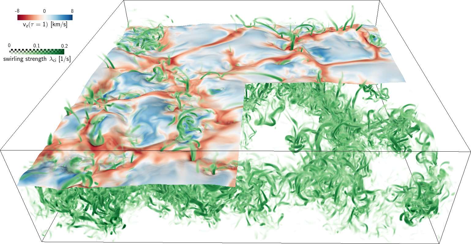
Figure 1: Snapshot of the swirling strength (green volume rendering) and the optical surface color-coded with vertical velocity (downflows in red and upflows in blue) in Run C. The size of the box shown is $4.8\times 4.8\times 1.4\,\mathrm{Mm^{3}}$. The optical surface is hidden in the lower right quadrant, uncovering the swirling structure in the subsurface layers.

2 Methods

2.1 Simulations of solar convection

Table 1: Parameters of the simulations. The vertical range is given with respect to the height at which the horizontal mean temperature is $\mathord{\approx}7000\,\mathrm{K}$.

Run	Box size [$\mathrm{Mm}^{3}$]	Cell size [$\mathrm{km}^{3}$]	Vertical range [km]
C	$4.86\times 4.86\times 1.4$	$7.5\times 7.5\times 10$	$-890<z<510$
D	$12\times 12\times 6.144$	$20.83\times 20.83\times 16$	$-5560<z<584$
H	$4.86\times 4.86\times 1.4$	$4\times 4\times 4$	$-884<z<516$

We used the MURaM code (Vögler 2003; Vögler et al. 2005) to solve the MHD equations in the context of solar surface convection, including radiative energy transfer and an equation of state which incorporates the effects of partial ionization. The simulations are performed on a Cartesian grid, using a 4th order central difference scheme for the spatial discretization and a short-characteristics scheme for the radiative transfer. At the bottom of the domain, open boundary conditions allow for the in- and outflow of matter: $\partial_{z}\@vec{v}=0$ for outflows and $v_{x,y}=\partial_{z}v_{z}=0$ for inflows, i.e., inflows are vertical. The pressure and the entropy of inflowing matter are chosen such that the total mass in the domain is approximately constant and the radiative energy loss is consistent with the solar luminosity. The top boundary is closed and the horizontal boundaries are periodic. The magnetic field is assumed to be vertical at the top and bottom boundaries: $B_{x,y}=\partial_{z}B_{z}=0$. For the radiative energy transfer, a gray approximation is assumed. The equation of state being used is appropriate for the conditions in the solar photosphere and the near-surface convection zone.

The parameters of the simulations considered here are listed in Table 1. Runs C and H cover the same vertical range at intermediate and high resolutions, respectively. Both simulations include weak, initially random magnetic fields and have previously been used to study near-surface dynamo action (Vögler & Schüssler 2007; Pietarila Graham et al. 2010; Moll et al. 2011). Their high resolution allows us to study the fine details of small vortices. Run D does not include a magnetic field and uses a lower resolution, allowing us to probe the convection zone at greater depths.

2.2 Vortex identification

Despite there being a clear intuitive notion of what a vortex is (viz., the rotation of fluid parcels about a possibly moving axis), it is surprisingly difficult to come up with a formal definition. In fact, contemporary research in fluid mechanics is still concerned with finding unambiguous vortex identification schemes (e.g., Haller 2005; Kolář 2007). Given its frequent use in the literature, it should be noted that a high vorticity $\omega=\left|\@vec{\nabla}\times\@vec{v}\right|$ is not a sufficient indicator for the presence of a vortex, because $\omega$ can also be high in shear flows without rotation.

To detect vortices, we use the so-called “swirling strength”, or $\lambda_{\mathrm{ci}}$, criterion (Zhou et al. 1999), which is based on an eigenanalysis of the velocity gradient tensor $U_{ij}\coloneqq(\partial_{j}v_{i})$. Vortices are defined to be regions where $U$ has a pair of complex conjugate eigenvalues. A large unsigned imaginary part $\lambda_{\mathrm{ci}}$ implies a region of “strong swirling”, i.e., (part of) a vortex. In the case of rigid rotation, the value of $\tau_{\mathrm{s}}\coloneqq 2\pi/\lambda_{\mathrm{ci}}$ gives the revolution period of the rotating flow. Unlike many other methods for vortex detection, the $\lambda_{\mathrm{ci}}$ criterion is applicable also in the case of compressible hydrodynamics (Kolář 2009).

Depending on the signs of the real eigenvalues $\lambda_{\mathrm{r}}$ and the real part of the complex eigenvalues $\lambda_{\mathrm{cr}}$, we discriminate four types of vortices (Haimes & Kenwright 1999):

1. $\lambda_{\mathrm{r}}<0$, $\lambda_{\mathrm{cr}}<0$: spiraling inward, converging

2. $\lambda_{\mathrm{r}}>0$, $\lambda_{\mathrm{cr}}<0$: spiraling inward, diverging

3. $\lambda_{\mathrm{r}}<0$, $\lambda_{\mathrm{cr}}>0$: spiraling outward, converging

4. $\lambda_{\mathrm{r}}>0$, $\lambda_{\mathrm{cr}}>0$: spiraling outward, diverging

Here, converging and diverging refer to the fluid motion along the direction of the eigenvector corresponding to $\lambda_{\mathrm{r}}$, which is identified as the direction of the vortex. Note that this direction is not necessarily orthogonal to the “swirling plane” spanned by the real and imaginary parts of the complex eigenvectors. We distinguish vortices by their inclination angle $\iota$ with respect to the vertical direction.

The identification of vortices via $\lambda_{\mathrm{ci}}$ is Galilean invariant, because it only relies on derivatives of the velocity field. Streamlines, however, are not invariant under Galilean transformations. Hence the streamlines in a particular frame of reference (e.g., the one which is at rest with respect to the computational box) do not always show circular orbits where vortices are detected. A strong vortex, however, is expected to produce vortical streamlines for a large range of observer velocities.

Although the definition of the swirling strength is purely local (as is the definition of vorticity), it can be shown that for a volume of rigidly rotating fluid, the swirling strength is uniform over the entire interior of the volume.

3 Results

3.1 Occurrence of vortices

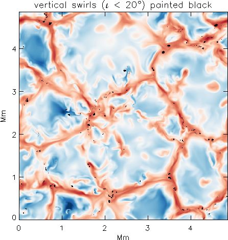
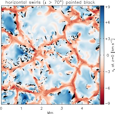
Figure 2: Vertical velocities at the average height of the optical surface ($T\approx 7000\,\mathrm{K}$). Black spots indicate vortices with a swirling period $\tau_{\mathrm{s}}<120\,\mathrm{s}$ and an inclination of less than $20^{\circ}$ with respect to the vertical (horizontal) direction in the left-hand (right hand) panel.

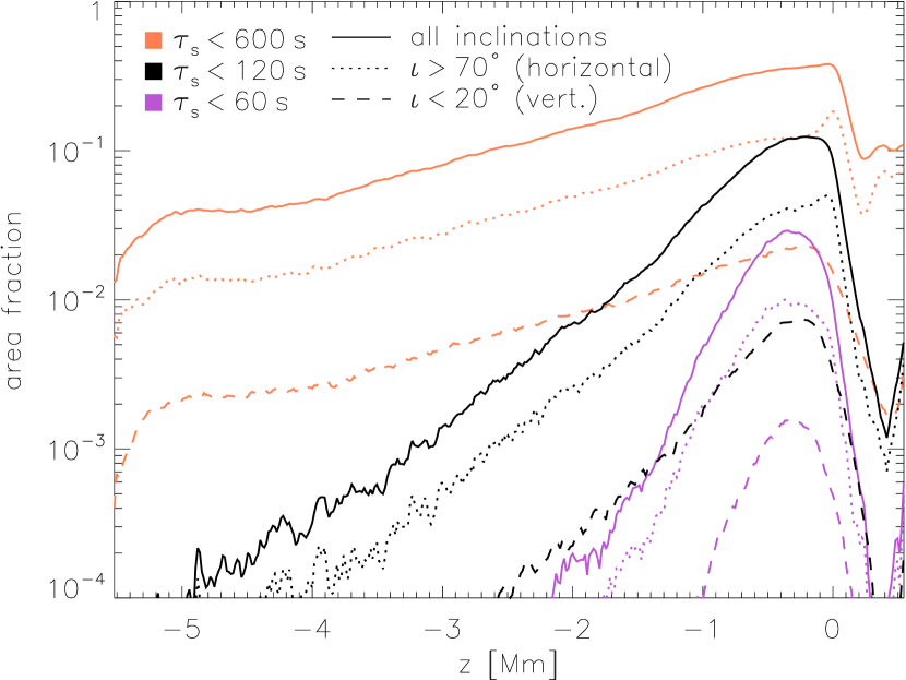
Figure 3: Horizontal area fraction of grid cells with swirling periods below a given threshold $\tau_{\mathrm{s}}$ as a function of height in Run D. $z=0$ corresponds to the average height of the optical surface.

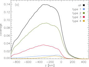
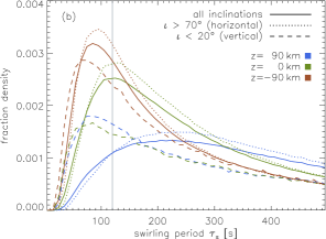
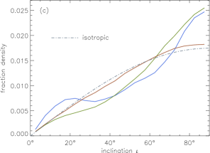
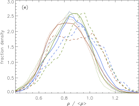
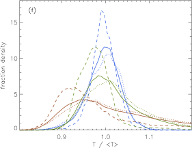
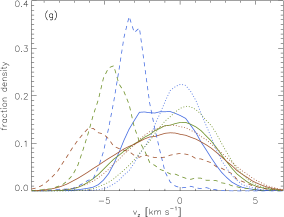
Figure 4: Vortex cell statistics for Run C. Except for panel (a), different heights are represented by brown ($z=-90\,\mathrm{km}$), green ($z=0$) and blue lines ($z=90\,\mathrm{km}$). Except for panel (b), only strong swirls with $\tau_{\mathrm{s}}<120\,\mathrm{s}$ are taken into account. The dashed and dotted lines represent the subset of vortices with vertical ($\iota<20^{\circ}$) and horizontal ($\iota>70^{\circ}$) orientation, respectively. The fraction densities plotted in panels (b)–(f) are normalized histograms, the normalization being such that the integral over all values of the respective abscissa variable is one. Angle brackets $\langle\ldots\rangle$ denote the horizontal mean of the respective variable in downflow regions (i.e., where $v_{z}<0$ at the respective height).

In all our simulations, the regions of strong swirl form a network of highly tangled filaments. An illustrative example of this is shown in Fig. 1. Some of the filaments protrude from the optical surface, forming variously shaped vortex tubes with different inclinations, sometimes bridging horizontally separated points in an arc. The optical surface is usually depressed at the footpoints of vertically emerging vortex tubes.

The horizontal distribution of the swirls is not homogeneous, the granular upflows being mostly devoid of them. Near the optical surface, vortices with a large inclination with respect to the vertical ($\iota>70^{\circ}$) are preferentially located at the edges of the intergranular downflow lanes, see Fig. 2. Those with a small inclination ($\iota<20^{\circ}$) are mostly inside the lanes where the downflow is strong.

We find most of the strong vortical flows at a few hundred kilometers below the optical surface, see Fig. 3. With an increasing upper limit for the swirling period, the distribution declines less steeply with depth, i.e., most of the very deep swirls are slow. The structure at great depths is also filamentary. Horizontal swirls (dotted lines) are more numerous than vertical ones (dashed lines), consistent with isotropy. Near and above the optical surface, the distribution of inclination angles deviates from isotropy (see next Section).

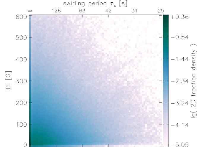
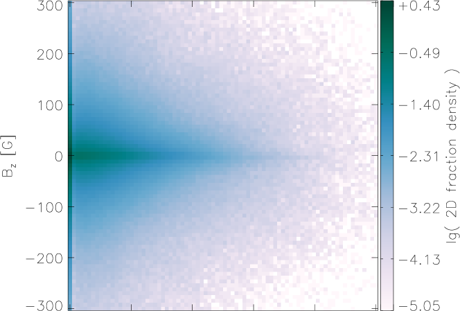
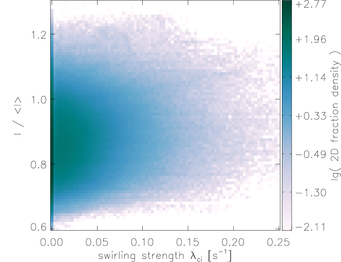
Figure 5: 2D histograms of the swirling strength and various observables (top panel: total magnetic field strength, middle panel: vertical magnetic field component, bottom panel: emerging intensity normalized by the overall horizontal mean) for Run C. All downflow regions in a $\pm 25\,\mathrm{km}$ range about the average height of the optical surface are taken into account. Each histogram is normalized such that an integral gives the fraction of volume with properties in the integrated range.

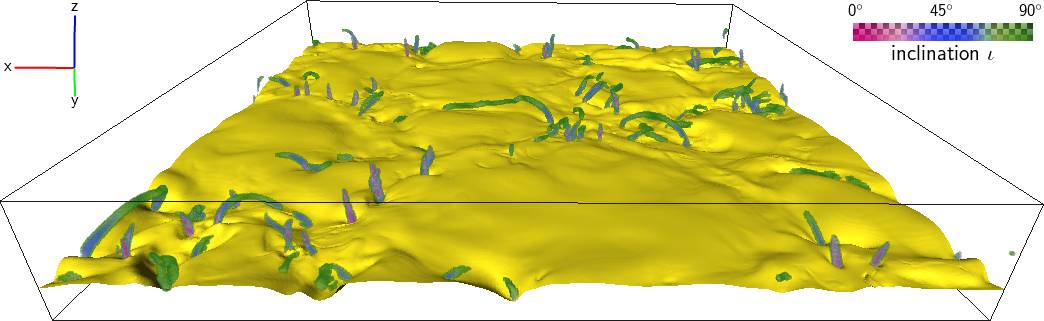
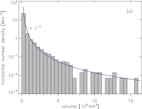
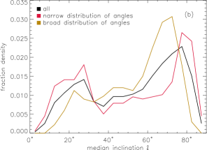
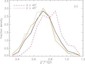
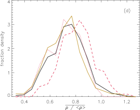
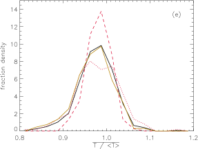
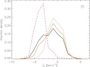
Figure 6: Snapshot of Run C with the warped optical surface in yellow and a volume rendering of the inclination angle $\iota$ in selected vortex features (see Sect. 3.3 for a description of the selection criteria). Pink and green colors correspond to vertically and horizontally oriented vortices, respectively. The size of the box shown is $4.8\times 4.8\times 0.7\,\mathrm{Mm^{3}}$.

Figure 7: Statistical properties of contiguous vortex features above the optical surface in Run C. The horizontal number density plotted in panel (a) is the number of features per horizontal area. In panels (b)–(f), features are classified by the median inclination $\hat{\iota}$ and the width of the distribution about the median. Vertical (horizontal) features are deemed to be those with narrow distributions and small (large) $\hat{\iota}$; they are represented by dashed (dotted) lines in panels (c)–(f). The plotted fraction densities are histograms normalized such that the integral over all values of the respective abscissa variable is one. In the abscissa labels, angle brackets $\langle\ldots\rangle$ denote the (height-dependent) horizontal mean of the respective quantity in downflow regions and a bar denotes the mean within a particular feature.

time: $0\,\mathrm{s}$
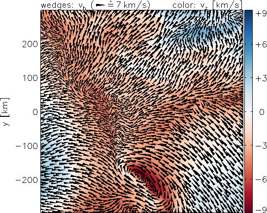
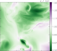
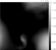
$50\,\mathrm{s}$
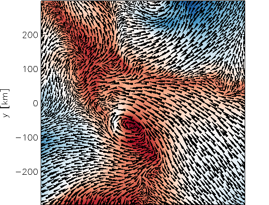
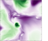
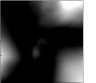
$126\,\mathrm{s}$

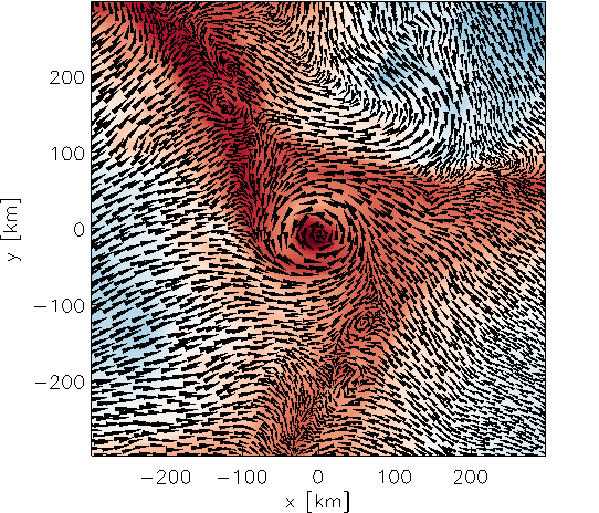
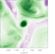
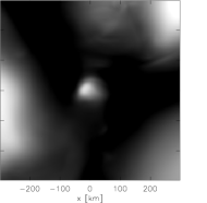
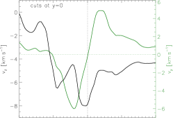
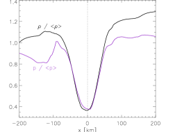
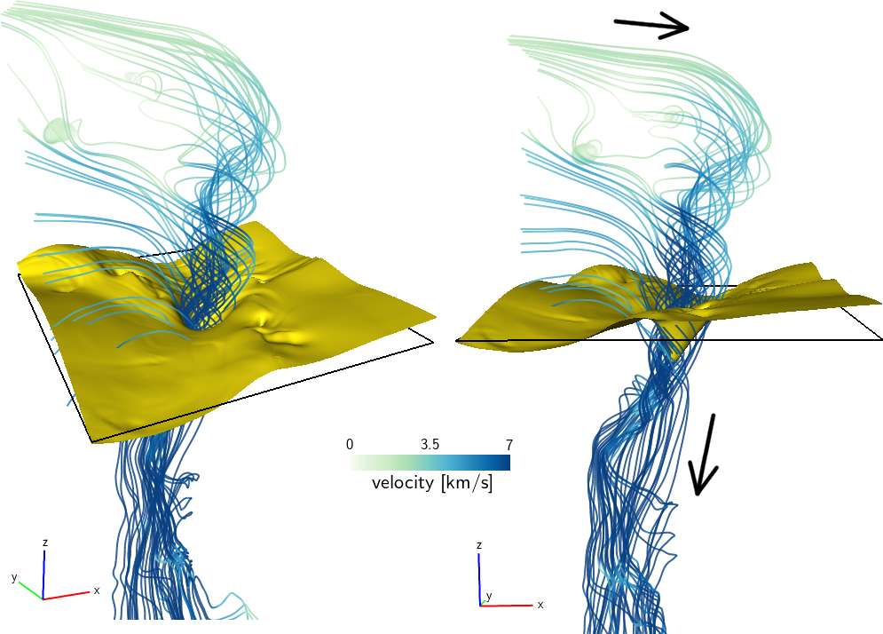
Figure 8: A strong vertical vortex penetrating the optical surface in Run H. The nine panels at the top show, at various stages of development, the velocity (left panels) and gas pressure (middle panels) at the average height of the optical surface ($z=0$) together with a bolometric intensity map (right panels). The line plots at the bottom left represent one-dimensional cuts through the vortex at the last instant ($t=126\,\mathrm{s}$). The 3D visualization at the bottom right shows, from two different viewing angles, selected streamlines color coded by velocity and the warped optical surface in yellow; the black rectangle indicates the $z=0$ plane.

3.2 Statistical properties of vortex regions

In Fig. 4, we present statistical properties of regions with large $\lambda_{\mathrm{ci}}$. For these analyses, we combined data from five different snapshots of Run C with a separation of about 7 minutes each. All grid cells are treated equally in the statistics, regardless of whether or not they form part of a larger, contiguous swirling region. In panels (b)–(h), we plot histograms normalized such as to give the fraction density with respect to the considered variable: the integral over a certain range of the variable gives the fraction of grid cells with values in that range. For every histogram we considered a $50\,\mathrm{km}$ (5 grid cells) vertical range about the indicated height, taking a total of $\mathrm{\sim}10^{7}$ grid cells into account. The individual panels of Fig. 4 are described in the following.

(a) This plot shows, as a function of height, the fraction of space occupied by swirls with $\tau_{\mathrm{s}}<120\,\mathrm{s}$ (compare Fig. 3). The highest occurrence of these swirls is at $z\approx-300\,\mathrm{km}$ ($z=0$ being the average height of the optical surface). Inwardly spiraling flows that diverge in the direction of the vortex (type 2, see Sect. 2.2) are prevailing everywhere; their mean fraction with respect to all types is 67% below $z=0$ and 75% above. The mean fraction of swirling flows of the outwardly spiraling, converging type (3) is 22% below $z=-200\,\mathrm{km}$ and decreases to 7% above $z=100\,\mathrm{km}$. Types (1) and (4) are insignificant.

(b) This plot shows histograms of the swirling period $\tau_{\mathrm{s}}$, normalized such that the integral over all $\tau_{\mathrm{s}}$ is one. The total fraction of grid cells with imaginary eigenvalues is about 53% at $z=-90\,\mathrm{km}$ and $z=0$, and 47% at $z=90\,\mathrm{km}$. With decreasing height, the histogram is more peaked and the peak moves toward larger swirling strengths (smaller $\tau_{\mathrm{s}}$). In all the other plots of Fig. 4, only strong swirls with $\tau_{\mathrm{s}}<120\,\mathrm{s}$ (i.e., to the left of the vertical line) are taken into account.

(c) The histograms of the inclination angle $\iota$ indicate that the swirls are preferentially (i.e., more than expected for an isotropic distribution) horizontal at $z=0$ and preferentially horizontal or vertical at $z=90\,\mathrm{km}$, whereas at $z=-90\,\mathrm{km}$ the distribution is consistent with an isotropic distribution (indicated by the gray dash-dotted line).

(d) The gas pressure $p$ in swirling regions is, on average, reduced to 87% of the horizontal mean $\langle p\rangle$ in all downflow regions ($v_{z}<0$) at the same height, consistent with a contribution by a dynamic pressure due to centrifugal forces. The gas pressure deficit does not depend much on height and inclination angle.

(e) The swirling regions are significantly rarefied, the average value of $\rho/\langle\rho\rangle$ being 84%. The rarefaction does not depend much on height and inclination angle.

(f) The mean of the relative temperature $T/\langle T\rangle$ is $1.0$ at all three considered heights. With increasing depth, the distribution becomes broader and the maximum moves towards lower temperatures. Most of the vertically oriented swirls (dashed lines) are slightly cooler than the horizontal ones (dotted lines), consistent with their predominant location inside cool intergranular lanes.

(g) In horizontal swirls (dotted lines), the median and the mean of the vertical velocity are near zero, in agreement with them being found at the edges of the granules. In vertical swirls (dashed lines), the mean is roughly $-3\,\mathrm{km\,s^{-1}}$ at all heights.

(h) The mean of the horizontal velocity $v_{\mathrm{h}}$ is approximately $3\,\mathrm{km\,s^{-1}}$, irrespective of the height. Note that this velocity includes the horizontal proper motion of the whole swirl. Vertical swirls tend to have slightly smaller horizontal velocities, presumably because most of them (being at the center of intergranular lanes) are not subject to the bulk motion of the expanding granules.

In Fig. 5, we present 2D histograms of the swirling strength and selected observables, taking into account all downflow regions near the optical surface. This restricts the analysis to the intergranular lanes. The top panel shows that strong magnetic fields become increasingly rare with increasing swirling strength, there being no apparent correlation between the two. This is also true for both polarities of the vertical magnetic field alone.

As is to be expected for the downflow lanes, the emerging intensity in vortex regions is preferentially smaller than the overall mean (bottom panel of Fig. 5). There is no clear trend towards higher intensity with increasing swirling strength. This indicates that, although vortices are locally bright, the contrast is small compared to the brightness variations within intergranular lanes.

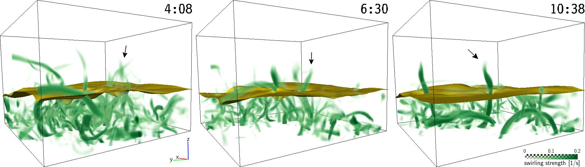
Figure 9: Formation of a strong vertical vortex in Run C. The plots display the swirling strength (green volume rendering) and the optical surface (yellow) at three different times (labels are in minutes). The size of the box shown is $1.1\times 1.1\times 0.8\,\mathrm{Mm^{3}}$.

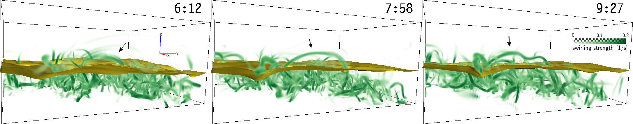
Figure 10: Rise and fall of a vortex arc in Run C. The plots display the swirling strength (green volume rendering) and the optical surface (yellow) at three different times (labels are in minutes). The size of the box shown is $1.5\times 1.5\times 0.8\,\mathrm{Mm^{3}}$.

3.3 Contiguous vortex features

We define vortex features to be contiguous regions of grid cells with a large swirling strength. To achieve a clear separation, we consider only features above the (warped) optical surface and take a lower cutoff for the swirling period than that used in the preceding section: $z>z(\tau=1)$ and $\tau_{\mathrm{s}}<60\,\mathrm{s}$. In 6 independent snapshots of Run C we find 3806 features that satisfy these criteria (this number includes isolated grid cells). The number of features decreases rapidly with size, see panel (a) of Fig. 7. It is roughly proportional to the inverse square of the occupied volume (blue line). In the following, we consider only the 622 features with at least 100 grid cells, corresponding to a minimum volume of $5.6\cdot 10^{4}\,\mathrm{km^{3}}$.

Fig. 7 shows the features detected in one of the snapshots. On visual inspection, we find that the inclination angle $\iota$ is in alignment with the longitudinal directions of the features, i.e., vertical (horizontal) features consist of swirls with small (large) inclination angles and more complicated shapes contain swirls with different inclinations. We use the median of the inclination angle $\iota$ as a characteristic value for each feature. This median is denoted with $\hat{\iota}$ in the following.

The histogram of $\hat{\iota}$ for all features is represented by the black line in panel (b) of Fig. 7. The red line represents the subset of features with a narrow distribution of angles, defined to be those for which 70% of all the constituent cells have an inclination $\iota$ within $\mathord{\pm}10^{\circ}$ about the feature’s median $\hat{\iota}$. The golden line represents all other features.

We divide the narrow subset (red) into two groups, a vertical one for which $\hat{\iota}$ is smaller than $45^{\circ}$ (dashed lines) and a horizontal one for which $\hat{\iota}$ is larger than $45^{\circ}$ (dotted lines). Density functions of the gas pressure, density, temperature and vertical velocity are plotted in panels (c)–(f); each quantity is divided by the horizontal mean in downflow regions at the respective height and then the mean within the respective feature is considered. The results are consistent with the “point-by-point” statistics presented in Sect. 3.2 (compare with Fig. 4): gas pressure and density are significantly reduced with respect to the horizontal mean, the differences between the horizontal and vertical subset being qualitatively similar. The vertical velocity is strongly negative (downward) in almost all of the vertical features.

Lifetimes

Through visual inspection, we estimate the lifetimes of 17 features in Run C. We define the lifetime to be the time interval in which a feature is visible as a distinct entity above the optical surface. The resulting mean lifetime is 3:30 minutes, the standard deviation being 1:40 minutes.

3.4 Individual examples and evolution

3.4.1 Vertical vortices

Fig. 8 displays an example of a vertically oriented vortex which penetrates the optical surface. Starting out as a somewhat distorted vortical flow (in the box’s frame of reference), it evolves into a roundish vortex with a diameter of approximately $80\,\mathrm{km}$. The rotation in the horizontal plane is nearly rigid at its core (innermost $60\,\mathrm{km}$) and the vertical velocity reaches a local maximum at the center of the vortex. Both gas pressure and density are lowered to as little as 36% of the respective horizontal mean at $z=0$ and are significantly distinct from the local background. The optical surface is depressed inside the vortex, the bottom of the depression being $110\,\mathrm{km}$ below $z=0$. At the site of the vortex, the bolometric intensity is locally increased by up to 24% with respect to the mean. The vortex thus appears as a bright spot within the dark intergranular lane.

Fig. 9 illustrates the formation of a vertical vortex. The feature is indicated by a black arrow in the three snapshots shown. It starts as a conglomeration of weakly swirling structures that apparently merge into a single distinct feature. The swirling strength increases with time. At all stages, the optical surface is depressed in the vortex, the largest depression being on the order of $\mathord{\sim}100\,\mathrm{km}$. Above the optical surface, the feature has a length of $\mathord{\sim}350\,\mathrm{km}$.

3.4.2 Vortex arcs

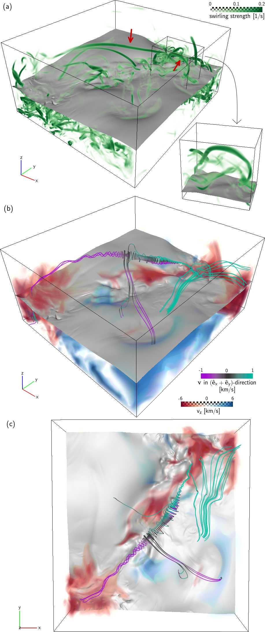
Figure 11: Snapshot of Run H with vortex arcs. All plots display the warped $\tau=1$ surface in gray color. Panel (a) shows the swirling strength (green volume rendering), red arrows indicate the features discussed in the text. Panels (b) and (c) show selected streamlines and the vertical velocity (red/blue volume rendering). The streamlines are colored according to the horizontal velocity in the approximate direction of the big arc. The size of the box shown is $1.3\times 1.4\times 0.7\,\mathrm{Mm^{3}}$. The blow-up in panel (a) contains the feature presented in Fig. 12.

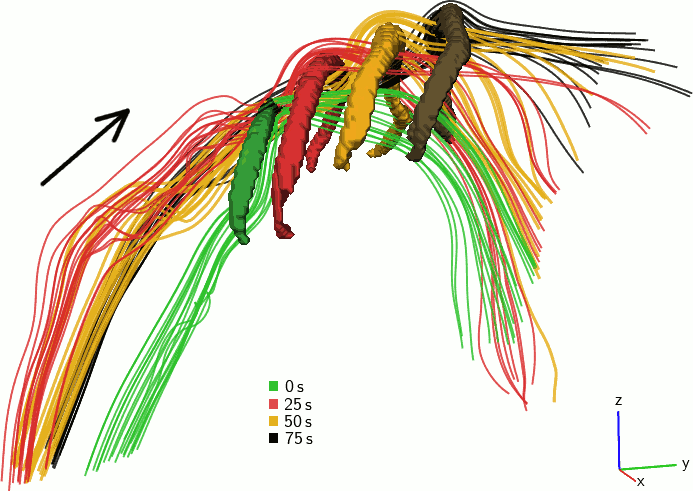
Figure 12: Evolution of the small vortex arc which is shown in a blow-up in Fig. 11. The isosurfaces show the arc at four different times with a separation of 25 seconds. For each stage, selected velocity streamlines are plotted in the corresponding color.

Fig. 10 displays the formation of a vortex arc. When the feature emerges through the optical surface, it is rather weak and hard to distinguish from the background. As it rises to its peak height, it gains in swirling strength. The horizontal distance between the two footpoints on the optical surface is $\mathord{\sim}780\,\mathrm{km}$ at this stage, the height above the surface is $\mathord{\sim}230\,\mathrm{km}$. At last, the feature develops a kink near its crest and collapses. In total, it lives for approximately 4 minutes.

Fig. 11 depicts a section from a snapshot of Run H which contains a big, slowly evolving vortex arc that hovers high above the optical surface. Next to it, on the right-hand side in the plots, is a much smaller and rapidly moving vortex arc. The two arcs are indicated with red arrows in panel (a). In the case of the big arc, the separation of the footpoints of the streamlines on the optical surface is $\mathord{\sim}1.4\,\mathrm{Mm}$, the peak height above the optical surface is $\mathord{\sim}330\,\mathrm{km}$. The vortical fluid motion, indicated by the large swirling strength in panel (a), is well visible in the streamlines plotted in panels (b) and (c). The purple and turquoise colors indicate the horizontal direction of the fluid motion: material flows from outside towards the big arc’s crest and down on both of its legs. At the part of the big arc where the streamlines are purple on one side and turquoise on the other, it is subject to longitudinal shear.

The small vortex arc has a horizontal extent of $\mathord{\sim}310\,\mathrm{km}$ and a peak height of $\mathord{\sim}210\,\mathrm{km}$ above the optical surface. Moving rapidly with respect to the computational frame of reference, it does not show vortical streamlines in panels (b) and (c) of Fig. 11. Its evolution is depicted in Fig. 12. In $75\,\mathrm{s}$, it propagates $\mathord{\sim}200\,\mathrm{km}$ horizontally and rises $\mathord{\sim}100\,\mathrm{km}$ vertically. The corresponding velocities are $2.7\,\mathrm{km\,s^{-1}}$ and $1.3\,\mathrm{km\,s^{-1}}$, respectively. The streamlines show that it corresponds to the front of an upward flow. In the upper, horizontal part of the arc, the mean density is reduced to 87% of the overall horizontal mean. A crude estimate of the buoyant rise velocity limited by aerodynamic drag (Eq. 6 in Parker 1975) yields $\mathord{\sim}1.6\,\mathrm{km\,s^{-1}}$. While this is consistent with the measured vertical velocity, it is not clear whether buoyancy plays an important active role in the vertical motion (cf. Arendt 1993).

3.5 Relationship with larger-scale vortical motion

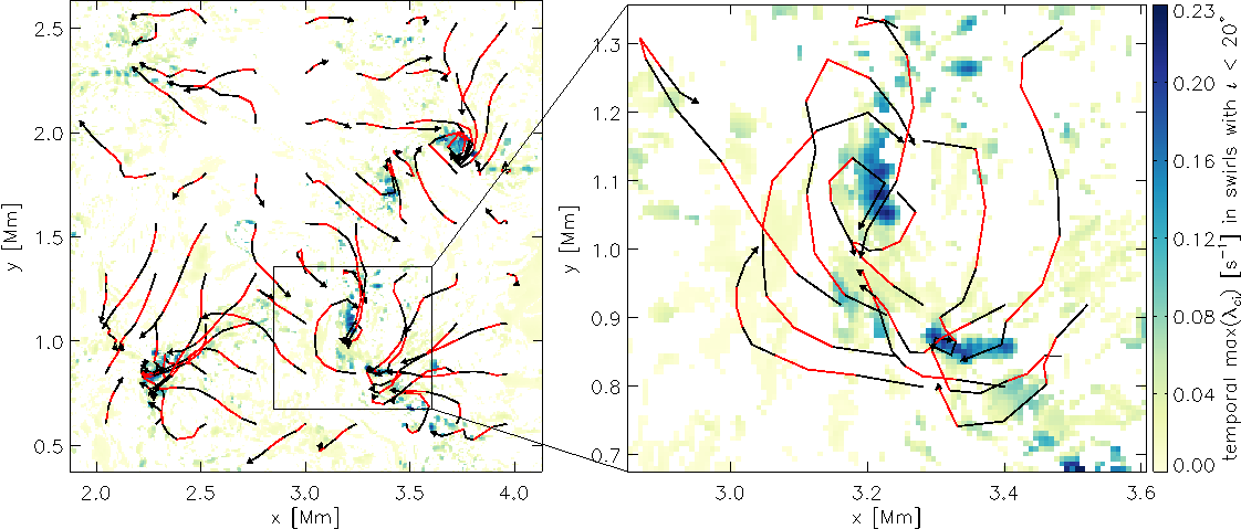
Figure 13: Horizontal pathlines in a 177 second time interval, plotted on top of a map of the temporal maximum of the swirling strength in vertically oriented swirls, at the average height of the optical surface. Each segment (black or red) of a pathline corresponds to 35 seconds.

As described in the introduction, observational evidence for vortical motion on the solar surface typically refers to larger scales than the strong, small-scale vortices studied here, although the general characteristics are similar (e.g., the association with downflows). The reported mean lifetimes of granular-scale vortices of 5–8 minutes (Bonet et al. 2008, 2010) are not drastically different from the value of $3.5\,\mathrm{min}$ estimated above. However, because their rotation periods are different, our vortices make about 2 revolutions during their lifetimes, while the observed vortices can be followed for only a fraction of one rotation (for instance, about 25% of a period in the case of Bonet et al. 2010). It is conceivable that the observed vortical motions represent the peripheral parts of the much stronger small-scale vortex cores that show up in the simulations but are too small to be observed directly. The outer vortex parts would be much more strongly affected by the evolving granulation pattern and thus be detectable only for a fraction of a rotation period.

To see whether the vortices studied in this paper would be detectable in observational data through feature tracking techniques, we consider horizontal pseudo pathlines (trajectories of fluid elements) in Fig. 13. The pathlines are determined from 10 snapshots of the horizontal velocity field at the average height of the optical surface with a temporal spacing of $\mathord{\approx}18\,\mathrm{s}$. They are “pseudo” because the vertical velocity is ignored.

Some pathlines are spiraling in towards a region of high swirling strength, see the feature at $(x,y)\approx(3.7,1.9)\,\mathrm{Mm}$ in the left-hand panel of Fig. 13. In this case, there is a clear association with the small-scale vortices presented in this paper. However, we also find pathlines which are curved but for which the association with an actual vortex is not clear, for instance in the blown-up region shown in Fig. 13.

4 Summary and discussion

We have investigated vortical fluid motions in simulations of near-surface solar convection by calculating the eigenvalues and eigenvectors of the velocity gradient tensor field. Complex eigenvalues with a large imaginary part indicate regions of strong swirling. They are found predominantly in and near the intergranular lanes, where cooled fluid is sinking down in a turbulent fashion. The swirling regions form an unsteady network of highly tangled filaments, some of which protrude above the optical surface.

Near the optical surface, vertically oriented swirls are preferentially located in the interior of intergranular lanes, where the downflow is strong. Horizontal swirls, on the other hand, are predominantly located at the edges of the granules, where vertical motion is mostly absent. The 3D structure of contiguous features above the optical surface is manifold, but often in the form of bent and arc-shaped filaments. These type of structures have previously been seen in independent numerical simulations with different codes, notably Muthsam et al. (2010) and Stein & Nordlund (1998). The swirling direction (rotation axis) is typically aligned with the longitudinal direction(s) in a contiguous feature.

Rotary motion causes dynamic pressure by centrifugal forces. One may, therefore, expect that vortex tubes are underdense as a result of pressure equilibrium and thermalization with the environment, analogous to magnetic flux tubes. We find vortex features above the optical surface to be underdense by $\mathord{\sim}15\%$ with respect to the horizontal mean in downflow regions. A significant depression of the optical surface is common where it intersects with vortices. Having diameters of $\mathord{\sim}80\,\mathrm{km}$, the largest vertical vortex features would be visible as bright spots with a size of $\mathord{\sim}0.1$ arcseconds in observations of the Sun.

Most vortex features are highly unsteady, being moved and/or twisted by turbulent fluid motions. Some of them rise upwards. Although, in principle, buoyancy could contribute to this rise (Parker 1991, but see also Arendt 1993) we find no unambiguous evidence for the operation of buoyancy forces. After a typical lifetime of a few minutes, the features usually descend below the optical surface, where they dissolve.

In general, the vortices presented here are smaller than those found in observations so far. They may represent peripheral parts of strong, small-scale vortices. However, arc-like motions of surface features do not necessarily imply the presence of a strong central vortex. The pattern of the fluid flow is changing considerably at time scales of only a few minutes, which is reflected by the lifetimes of the small-scale vortices. We therefore reckon that granular-scale or bigger vortical flows are less numerous than small-scale vortices.