Bayesian hierarchical modeling for signaling pathway inference from single cell interventional data

Abstract

Recent technological advances have made it possible to simultaneously measure multiple protein activities at the single cell level. With such data collected under different stimulatory or inhibitory conditions, it is possible to infer the causal relationships among proteins from single cell interventional data. In this article we propose a Bayesian hierarchical modeling framework to infer the signaling pathway based on the posterior distributions of parameters in the model. Under this framework, we consider network sparsity and model the existence of an association between two proteins both at the overall level across all experiments and at each individual experimental level. This allows us to infer the pairs of proteins that are associated with each other and their causal relationships. We also explicitly consider both intrinsic noise and measurement error. Markov chain Monte Carlo is implemented for statistical inference. We demonstrate that this hierarchical modeling can effectively pool information from different interventional experiments through simulation studies and real data analysis.

TITL1Supported in part by National Science Foundation Grant DMS-07-14817, National Heart, Lung, and Blood Institute Contract N01 HV28186, National Institute of Drug Abuse Grant P30 DA018343, National Institute of General Medical Sciences Grant R01 GM59507, Yale University Biomedical High Performance Computing Center and NIH Grant RR19895, which funded the instrumentation.

and

1 Introduction

Cells respond to internal and external changes through signaling networks. One major research area in biology is to identify signaling proteins and understand how they coordinate to function properly. With recent technological advances in genomics and proteomics, researchers now can monitor and quantify molecular activities at the genome level, making it possible to reconstruct signaling pathways from these high-throughput data. Although efforts have been made to use microarray gene expression data and sequence data to reveal signaling pathways [e.g., Liu and Ringnér (2007)], these data are limited in two important aspects. First, signaling pathways function at the protein level, so measured gene expression levels from microarrays at most can provide a proxy to the protein activity levels. Second, each cell may behave differently from other cells due to complex interactions among many proteins, some substantially. Therefore, population level data collected by microarrays can mask individual cell differences, making it difficult to infer underlying pathways. In contrast, single cell level protein activity data offer much richer information for pathway inference.

Flow cytometry [Herzenberg et al. (2002); Perez and Nolan (2002)] is a powerful fluorescence-based technology that can make rapid, sensitive, and quantitative measurements of multiple proteins for thousands of individual cells. It can measure both a specific protein’s expression level and protein modification states such as phosphorylation. Therefore, phospho-protein responses to environmental stimulations can be monitored at the single cell level for thousands of cells very efficiently, and this technology has been employed to infer signaling pathways through gathering activity levels of multiple proteins under different stimulatory or inhibitory conditions [Sachs et al. (2005)]. We focus on the analysis of single cell flow cytometry data in this article.

Several methods have been applied for network inference based on genomics data, including Bayesian Networks (BNs) [Pe’er et al. (2001); Pe’er (2005)], Markov Networks (MNs, also called Markov random fields) [Wei and Li (2007, 2008)], and Dependency Networks (DNs) [Heckerman et al. (2000)]. Common to all these methods, each protein (or gene) is represented by a node and a dependency between two proteins is represented by an edge in the network. More formally, we define a graph $\mathcal{G}=(V,E)$ with its nodes $V=\{1,\ldots,P\}$ and an edge set $E$. We use $X_{i}$ to refer to the value of the $i$th node, that is, the expression level of the $i$th protein. The methods differ in how the edges are inferred from the observed data. In BN, the network is a directed acyclic graph where the state of each node only depends on its immediate ancestors. This structure imposes Markovian dependency among all the nodes stating that each variable is conditionally independent of its nondescendants given its parent variables. So the joint likelihood for all the nodes, that is, proteins, can be factored into a product of conditional probabilities. BNs pose significant computational challenges to learn the network structure because the model space to be explored is super-exponential in the number of genes to be studied. More recently, Ellis and Wong (2008) proposed a method to reduce the bias in the fast mixing algorithm proposed by Friedman and Killer (2003) to sample the BN structures from the posterior distribution. MNs are undirected graphical models and are similar to BNs in representation of dependencies: each random variable is conditionally independent of all other variables given its neighbors. Gaussian Graphical Models (GGMs) [Lauritzen (1996); Schäfer and Strimmer (2005); Dobra et al. (2004)], a subclass of MNs, assume a multivariate normal distribution as the joint distribution of random variables. The existence of an undirected edge in a GGM is implied by the nonzero partial correlation coefficient derived from the precision matrix. Some studies have found that BNs outperform GGMs in inferring networks based on interventional data where the biological system is perturbed through designed experiments, but GGMs may perform better for observational data, for example, Werhli, Grzegorczyk and Husmeier (2006). DNs aim to reduce computational burden where a large number of genes are modeled by building a collection of conditional distributions separately. DNs define the conditional distributions $\{p(X_{i}|X_{-i})\}$ separately for each $X_{i}$. When we focus on sparse normal models, DNs define a set of $P$ separate conditional linear regression models in which $X_{i}$ is regressed on a small selected subset of predictor variables, which are determined separately.

Because a statistical association between two variables only implies association not causation, standard DN and GGM approaches cannot be used to infer causal networks, a goal in signaling pathway analysis. In this article we develop a Bayesian hierarchical modeling approach based on DNs to address this limitation. This is achieved through appropriate intervention experiments to dissect directional influences. To accommodate varying relationships among proteins under different experimental conditions, we allow a different set of regression models for each condition. At the same time, the hierarchical framework imposes similar functional forms across conditions to borrow information from different experiments. As for causal inference, the basic idea is that for any protein $i$, its regulators exert similar effects if it is not intervened, and would have no effect when $i$ is controlled. In contrast to standard regression models where the predictors are assumed to be error-free, our model allows measurement errors in predictor variables.

A large part of the difficulty in the standard BN computation is due to the requirement that the network be acyclic. Our approach is not guaranteed to give acyclic networks. However, in terms of sensitivity and specificity to detect true edges, our method is competitive with the best methods that impose the acyclic graph assumption. This is illustrated by our results in the example of Sachs et al. (2005).

The paper is organized as follows. In Section 2 we describe two hierarchical models (a general hierarchical model where no constraints are imposed and a restricted hierarchical model where a symmetry constraint is imposed) and the methods for statistical inference of the network. For comparison, we also describe a nonhierarchical model where all the experiments are pooled together for analysis. Then we investigate the performance of these methods on simulated data in Section 3. In Section 4 we apply these methods to data from a study of the signaling networks of human primary naive CD4⁺ cells [Sachs et al. (2005)]. We finish the paper with discussions in Section 5.

2 Methods

The primary goal of our statistical model is to infer causal influences among proteins from interventional data. In this section we describe three models: a hierarchical model (HM), a restricted hierarchical model (RHM), and a nonhierarchical model (NHM), that can be used to infer the relationships among proteins. We also discuss statistical methods to infer causal networks in this section.

2.1 Hierarchical model (HM)

First we discuss a Bayesian hierarchical model to infer the relationships among proteins both at the overall level across all experiments and under individual experimental conditions. Our model incorporates both measurement errors and the intrinsic noises due to the biological process and unmodeled biological variations.

Let $P$ denote the number of proteins, $K$ denote the number of experimental conditions, and $N_{k}$ denote the number of samples (individual cells) under the $k$th condition, $k=1,2,\dots,K$. We further let $\tilde{x}_{\mathit{ink}}$ denote the true activity level of the $i$th protein in the $n$th cell under the $k$th experimental condition, and $x_{\mathit{ink}}$ the measured value of its activity, where $x_{\mathit{ink}}=\tilde{x}_{\mathit{ink}}+\varepsilon^{M}_{\mathit{ink}}$, and the measurement error $\varepsilon^{M}_{\mathit{ink}}$ is a normal random variable with mean 0 and standard deviation $\sigma^{M}$, that is, $\varepsilon^{M}_{\mathit{ink}}\sim\mathrm{N}(0,(\sigma^{M})^{2})$. Our model assumes that there exists a linear relationship among the activity levels of proteins. That is, for each protein $i=1,2,\dots,P$ and for each condition $k=1,2,\dots,K$,

$$\tilde{x}_{\mathit{ink}}=\alpha_{i0}^{(k)}+\sum_{j\neq i}{\alpha_{ij}^{(k)}\tilde{x}_{\mathit{jnk}}}+\varepsilon_{\mathit{ink}}^{I},$$ (1)

where $\varepsilon_{\mathit{ink}}^{I}$ is the intrinsic noise and has a normal distribution $\mathrm{N}(0,(\sigma^{I}_{i})^{2})$. We assume that the error terms $\{\varepsilon_{\mathit{ink}}^{I}\}$ are independent, and are independent of the measurement errors $\{\varepsilon^{M}_{\mathit{ink}}\}$. In equation (1), $\alpha_{ij}^{(k)}=0$ if there is no linear relationship between the activity levels of proteins $i$ and $j$ under the $k$th experimental condition. A nonzero value of $\alpha_{ij}^{(k)}$ implies the existence of a linear relationship (but not necessarily a causal effect). To correctly infer the network among these proteins, we need to first find, for each protein, the subset of proteins that are linearly associated with its expression level, which is implied by the set of nonzero coefficients in (1). The linear relationship among the true expression values $\tilde{x}_{\mathit{ink}}$ implies that the observed values are also linearly related:

$$x_{\mathit{ink}} = \alpha_{i0}^{(k)}+\sum_{j\neq i}{\alpha_{ij}^{(k)}(x_{\mathit{jnk}}-\varepsilon^{M}_{\mathit{jnk}})}+\varepsilon^{I}_{\mathit{ink}}+\varepsilon_{\mathit{ink}}^{M}$$

$$= \alpha_{i0}^{(k)}+\sum_{j\neq i}{\alpha_{ij}^{(k)}x_{\mathit{jnk}}}+\varepsilon^{I}_{\mathit{ink}}+\varepsilon_{\mathit{ink}}^{M}-\sum_{j\neq i}\alpha_{ij}^{(k)}\varepsilon^{M}_{\mathit{jnk}}.$$

Comparing (1) and (2.1), we can see that correctly inferring the relationship in the network depends on the correct inference of the set of nonzero coefficients in (2.1).

For each protein, we utilize indicator variables $z_{ij}=0$/1 to denote the relationship between proteins $i$ and $j$ such that $z_{ij}=1$ if and only if the coefficient of the $j$th protein in the regression model for the $i$th protein is nonzero. The values of $z_{ij}$ may differ under different experimental conditions. For example, if protein $j$ regulates protein $i$, $z_{ij}=1$ when $i$ is not controlled and the association strength between the two proteins should be similar under such conditions. However, $z_{ij}=0$ when $i$ is controlled because the relation between $X_{i}$ and $X_{j}$ is destroyed. Therefore, it is natural to use a hierarchical structure to formalize this thinking. We use $w_{ij}^{(k)}$ to denote the probability that $z_{ij}=1$, that is, protein $j$ is related to protein $i$ under the $k$th experimental condition. The prior we take for the regression coefficient $\alpha_{ij}^{(k)}$ is a mixture of two distributions. One is a point mass at zero, indicating that the $j$th protein is not linearly related to the $i$th protein under the $k$th condition. The other is a normal distribution for nonzero effects, with weight $w_{ij}^{(k)}$. Specifically, the prior for the slope coefficient $\alpha_{ij}^{(k)}$ ($j\neq i$) is

$$\alpha_{ij}^{(k)}|w_{ij}^{(k)},\alpha_{ij},\sigma^{\alpha}_{ij}\sim\bigl{(}1-w_{ij}^{(k)}\bigr{)}\delta_{0}\bigl{(}\alpha_{ij}^{(k)}\bigr{)}+w_{ij}^{(k)}\mathrm{N}\bigl{(}\alpha_{ij}^{(k)}|\alpha_{ij},(\sigma^{\alpha}_{ij})^{2}\bigr{)},$$ (3)

where $\delta_{0}(\cdot)$ indicates a point-mass at zero, and $w_{ij}^{(k)}$ is the probability that $\alpha_{ij}^{(k)}\neq 0$. When $\alpha_{ij}^{(k)}\neq 0$, the prior for $\alpha_{ij}^{(k)}$ is $\mathrm{N}(\alpha_{ij},(\sigma^{\alpha}_{ij})^{2})$ with a common mean and a common standard deviation across different experimental conditions. Under this setup, information is shared for coefficients $\alpha_{ij}^{(k)}$ across different conditions. Similarly, we borrow information for $w_{ij}^{(k)}$ across different experimental conditions by applying a beta distribution as a prior for $w_{ij}^{(k)}$ with a common mean $w_{ij}$ and a common variance $w_{ij}(1-w_{ij})/(v_{ij}+1)$:

$$w_{ij}^{(k)}|w_{ij},v_{ij}\sim\operatorname{Beta}\bigl{(}w_{ij}v_{ij},(1-w_{ij})v_{ij}\bigr{)}.$$ (4)

So $w_{ij}^{(k)}$ measures the probability that there is an association between proteins $i$ and $j$ under the $k$th experimental condition, and $w_{ij}$ measures the overall-level probability that the two proteins are associated.

To complete the model, we specify a beta distribution $\operatorname{Beta}(\beta_{1},\beta_{2})$ for $w_{ij}$, a normal distribution $\mathrm{N}(a^{(i)},\tau^{(i)})$ for $\alpha_{ij}$ and gamma distributions: $\mathrm{G}(\gamma_{1},\gamma_{2})$, $\mathrm{G}(\gamma_{3},\gamma_{4})$ and $\mathrm{G}(\gamma_{5},\gamma_{6})$ for $(\sigma_{i}^{I})^{-2}$, $(\sigma^{\alpha}_{ij})^{-2}$ and $(\sigma^{M})^{-2}$, as their respective prior distributions. In the simulation studies, we take $\gamma_{i}=\beta_{j}=1$ for $i=1,2$ and $j=1,2,\ldots,6$, $a^{(i)}=0$ and $\tau^{(i)}=1000$ for $i=1,\ldots,P$. In real data analysis, we vary the hyperparameter values to study the sensitivity of the inference results to these values. We note that the posterior distribution is proper since we take proper priors for all the parameters.

One attractive feature of this model is that when $w_{ij}^{(k)}$ is integrated out, the marginal distribution of $\alpha_{ij}^{(k)}$ is independent of $v_{ij}$:

$$\alpha_{ij}^{(k)}|w_{ij},\alpha_{ij},\sigma^{\alpha}_{ij}\sim(1-w_{ij})\delta_{0}\bigl{(}\alpha_{ij}^{(k)}\bigr{)}+w_{ij}\mathrm{N}\bigl{(}\alpha_{ij}^{(k)}|\alpha_{ij},(\sigma^{\alpha}_{ij})^{2}\bigr{)}.$$ (5)

Given $\alpha_{ij}^{(k)}$ and $w_{ij}$, when $v_{ij}$ is specified, the posterior distribution of $w_{ij}^{(k)}$ is

$$w_{ij}^{(k)}|w_{ij},v_{ij},\alpha_{ij}^{(k)}\sim\operatorname{Beta}\bigl{(}w_{ij}v_{ij}+I\bigl{(}\alpha_{ij}^{(k)}\neq 0\bigr{)},(1-w_{ij})v_{ij}+I\bigl{(}\alpha_{ij}^{(k)}=0\bigr{)}\bigr{)}.$$ (6)

Hence, we can first sample the posterior distributions of $\alpha_{ij}^{(k)}$ and $w_{ij}$, and then sample $w^{(k)}_{ij}$ according to equation (6).

Under this model, the inference of the causal network consists of two steps. First, based on the posterior means $\hat{w}_{(i,j)}$ of the overall-level probability $0.5\times(w_{ij}+w_{ji})$, we infer whether there is an association between proteins $i$ and $j$ with a certain threshold $u_{1}$. Second, for each pair of proteins $(i,j)$ that are inferred to be associated, we determine their regulatory direction based on the experiment-level probabilities $w^{(k)}_{ij}$ to infer the causal network. The underlying assumption of our inference is that for a pair of proteins ($i$ and $j$) that has a regulatory relation, say, $i$ regulates $j$ ($i\rightarrow j$), controlling (inhibiting or activating) over protein $j$ affects the activity of $j$ but not $i$, resulting in much reduced or lack of association between $i$ and $j$; controlling over protein $i$ affects the activity of $i$ and hence $j$, keeping the association between them. The posterior distributions of $w^{(k)}_{ij}$ given $\alpha_{ij}^{(k)}$ and $w_{ij}$, with $v_{ij}$ prespecified, is given in equation (6). To better reflect the changes of $w^{(k)}_{ij}$ for different $k$, we use $v_{ij}\equiv 0.1$ in our analysis, because larger values of $v_{ij}$ (e.g., 10) are not able to reveal the changes in $w^{(k)}_{ij}$, as the parameters in (6) are dominated by $v_{ij}$ when $v_{ij}$ is large, and $I(\alpha^{(k)}_{ij}\neq 0)$ plays a smaller role in (6). To put this into more concrete terms, we consider $w_{ij}=0.9$ as an example, which gives a strong support for the association between proteins $i$ and $j$. The difference between the distributions $\operatorname{Beta}(0.9\times 10+1,0.1\times 10)$ and $\operatorname{Beta}(0.9\times 10,0.1\times 10+1)$ when $v_{ij}=10$ is much less than that between $\operatorname{Beta}(0.9\times 0.1+1,0.1\times 0.1)$ and $\operatorname{Beta}(0.9\times 0.1,0.1\times 0.1+1)$ when $v_{ij}=0.1$.

To determine the directions of edges, we calculate the posterior means $\hat{w}^{(k)}_{ij}$ of $w^{(k)}_{ij}$ for all $k$ and $(i,j)$ pairs. For each pair $(i,j)$, if all the values in a stream (e.g., $\{\hat{w}^{(k)}_{ji}\}_{k}$) are small (less than a threshold $u_{2}>0$, so the signal in this stream is weak compared to noises), then we ignore this stream and infer the causal relations only based on the other one ($\{\hat{w}^{(k)}_{ij}\}_{k}$). The inference is based on checking whether $\hat{w}^{(k)}_{ij}$ under specific conditions decreases greatly compared to the highest value. Let $S_{i,j}=\{k:k\in\{i,j\}\}$ denote the set of conditions under which $i$ or $j$ is perturbed, and $|S_{i,j}|$ be its cardinality. We propose the following four criteria to determine the causal relationship between an associated protein pair ($i$, $j$):

=335pt Stimulus Effect 1 CD3, CD28 general perturbation 2 ICAM2 general perturbation 3 Akt-inhibitor Inhibits Akt 4 G0076 Inhibits Pkc 5 Psi Inhibits Pip2 6 U0126 Inhibits Mek 7 Ly Inhibits Akt 8 PMA Activates Pkc 9 $\beta_{2}c\mathit{AMP}$ Activates Pka

Table 1: A summary of the nine experimental conditions for the data in Sachs et al. (2005)

• Case 1: $|S_{i,j}|=1$, that is, $i$ or $j$ is only perturbed in one condition. Without loss of generality, we suppose that protein $i$ is controlled under condition $k^{\prime}$ ($S_{i,j}=\{k^{\prime}\}$). If $\max_{k}\{\hat{w}^{(k)}_{ij}\}-\hat{w}^{(k^{\prime})}_{ij}>u_{3}$ for a threshold $u_{3}>0$, then from stream $\{\hat{w}^{(k)}_{ij}\}_{k}$ we infer $j\rightarrow i$. Otherwise, we infer $i\rightarrow j$. Similarly, we make an inference from the stream $\{\hat{w}^{(k)}_{ji}\}_{k}$. If the directions inferred from both streams are the same, say, $i\rightarrow j$, we infer that direction as the direction of the edge between $i$ and $j$: $i\rightarrow j$. If the directions from both streams are different, we say that the direction of the edge is undetermined. Taking the conditions in Table 1 for the network in Figure 1 as an example, pairs $(1,2)$, $(1,8)$, $(2,6)$ $(3,4)$, $(4,5)$, $(6,8)$, $(8,10)$, and $(8,11)$ belong to Case 1.

• Case 2: $|S_{i,j}|>1$ and for all $k\in S_{i,j}$, the same protein, say, $i$, is controlled. For each stream, for example, $\{\hat{w}^{(k)}_{ij}\}_{k}$, if $\max_{k}\{\hat{w}^{(k)}_{ij}\}-\hat{w}^{(k^{\prime})}_{ij}>u_{3}$ for all $k^{\prime}\in S_{i,j}$, then we infer $j\rightarrow i$; if $\max_{k}\{\hat{w}^{(k)}_{ij}\}-\hat{w}^{(k^{\prime})}_{ij}\leq u_{3}$ for all $k^{\prime}\in S_{i,j}$, then we infer $i\rightarrow j$; otherwise, we do not infer a direction from this stream. If both streams lead to a directional inference and the directions are the same (Figure 4, top panel), or if only one stream provides a directional inference, then we infer the direction of the edge. Otherwise, the direction is undetermined. For the conditions in Table 1, pairs $(1,9)$, $(3,9)$, $(5,7)$ $(6,7)$, $(9,10)$, $(9,11)$ belong to Case 2.

• Case 3: $|S_{i,j}|>1$ and both proteins are controlled in the experiments. Let $S_{i,j}^{(i)}$ denote the set of conditions under which protein $i$ is controlled, and $S_{i,j}^{(j)}$ the set of conditions under which protein $j$ is controlled. For each stream, for example, $\{\hat{w}^{(k)}_{ij}\}_{k}$, we calculate the differences of $\hat{w}^{(k)}_{ij}$ when $i$ or $j$ is controlled: $d^{(k_{1}k_{2})}_{ij}=\hat{w}^{(k_{1})}_{ij}-\hat{w}^{(k_{2})}_{ij}$ for each $k_{1}\in S_{i,j}^{(i)}$ and $k_{2}\in S_{i,j}^{(j)}$. If $d^{(k_{1}k_{2})}_{ij}>u_{3}$ for all $k_{1}\in S_{i,j}^{(i)}$ and $k_{2}\in S_{i,j}^{(j)}$, we infer that $i\rightarrow j$; if $d^{(k_{1}k_{2})}_{ij}\leq-u_{3}$ for all $k_{1}\in S_{i,j}^{(i)}$ and $k_{2}\in S_{i,j}^{(j)}$, we infer that $j\rightarrow i$; otherwise, the direction is undetermined from this stream. If both streams lead to a directional inference and the directions are the same, or if only one stream provides a directional inference, then we infer the direction of the edge. Otherwise, the direction is undetermined. For the conditions in Table 1, pairs $(2,9)$, $(4,9)$, $(7,8)$ $(8,9)$ belong to Case 3.

• Case 4: $|S_{i,j}|=0$, that is, no perturbation is conducted on either protein. In this case, we cannot infer the causal relation.

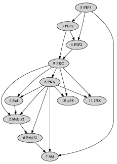
Figure 1: Pathway adapted from Sachs et al. (2005) by including three missed edges and correcting one reversed edge. Nodes represent proteins, and directed edges represent signal transduction.

The choices of the thresholds $u_{1}$, $u_{2}$, and $u_{3}$ will be discussed in simulation studies. Generally speaking, the two steps involved in causal network inference are based on the posterior distributions of $w_{ij}$ and $w_{ij}^{(k)}$. The overall-level probability $w_{ij}$ measures the strength of the linear relationship between two proteins across all the conditions. Based on $w_{ij}$, we infer the set of proteins that are related from which we determine an undirected graph. The changes in the experiment-level probabilities $w_{ij}^{(k)}$ offer insights on the directions of causal regulations.

2.2 Restricted hierarchical model (RHM)

The $w_{ij}$ and $w_{ij}^{(k)}$ in (3), (4), and (6) denote the probability that protein $j$ is included in the linear model to predict the activity level of protein $i$ across all the experiments and under the $k$th specific condition, respectively. In this framework, we may impose the constraint that $w_{ji}=w_{ij}$ and $w_{ji}^{(k)}=w_{ij}^{(k)}$ for each $k$, that is, the existence of a linear relationship between proteins $i$ and $j$ is independent of which variable is the predictor and which is the response variable. We can infer the posterior distributions of $w_{ij}$ and $w_{ij}^{(k)}$ under this constraint, and call this model a restricted hierarchical model (RHM). Based on the posterior means of $w_{ij}$, we can infer whether proteins $i$ and $j$ are associated with each other by setting up an appropriate threshold $u^{\prime}_{1}$. For each associated pair, we can infer the causal relationship according to the changes in $w_{ij}^{(k)}$. The choice of the threshold will be illustrated in Section 3.1 and Supplementary Material S3 [Luo and Zhao (2010)] details the criteria in determining the causal relations for the associated pairs of proteins. Different from HM, we must prespecify $v_{ij}$ in RHM to sample from the posterior distributions of $w_{ij}$ and $w_{ij}^{(k)}$. We will show how different values of $v_{ij}$ affect the network inference in the following discussion.

2.3 Nonhierarchical model (NHM)

To demonstrate the usefulness of the hierarchical model approach, we also consider a nonhierarchical model (NHM) as a reference model for comparisons. The NHM assumes a linear model among the activity levels of proteins and incorporates both measurement errors and intrinsic noises as in equation (2.1). The main difference is that this NHM assumes identical regression coefficients across different experimental conditions:

$$x_{\mathit{ink}}=\alpha_{i0}+\sum_{j\neq i}{\alpha_{ij}x_{\mathit{jnk}}}+\varepsilon_{\mathit{ink}}^{I}+\varepsilon_{\mathit{ink}}^{M}-\sum_{j\neq i}\alpha_{ij}\varepsilon^{M}_{\mathit{jnk}},$$ (7)

where the intrinsic noise $\varepsilon_{\mathit{ink}}^{I}$ follows the normal distribution $\mathrm{N}(0,(\sigma_{i}^{I})^{2})$, the measurement error $\varepsilon_{\mathit{ink}}^{M}$ follows the normal distribution $\mathrm{N}(0,(\sigma^{M})^{2})$, and they are assumed to be independent. As in HM, we also apply mixture distributions as priors for the coefficients $\alpha_{ij}$:

$$\alpha_{ij}\sim(1-w_{ij})\delta_{0}(\alpha_{ij})+w_{ij}\mathrm{N}(\alpha_{ij}|a,\tau^{2}).$$ (8)

The posterior distributions of $w_{ij}$ provide information about whether proteins $i$ and $j$ are associated. However, it is impossible to make causal inference from this model.

For all three models, we use MCMC methods to sample the posterior distributions. Supplementary Material S2 [Luo and Zhao (2010)] provides details of the MCMC updates for HM. The MCMC updates for RHM and NHM are similar and not shown in this paper.

3 Simulation study

We first apply our methods to simulated data to illustrate how to infer the causal network from the posterior distributions of the overall-level probabilities $w_{ij}$ and the experiment-level probabilities $w_{ij}^{(k)}$, for both HM and RHM. We also study how the inference differs between these two methods and for different choices of $v_{ij}$. We then study the performance of our methods on simulated data with heavy tail distributed intrinsic noises.

We simulate data based on the network shown in Figure 1, which is adapted from Sachs et al. (2005) by correcting one reversed edge and including three missed edges. From Figure 1, we can derive the parent set for each node (protein). For any protein $i$, we first generate the association strength $\alpha_{ij}$ from the uniform distribution over the interval $[0.5,2]$, and randomly assign the sign of $\alpha_{ij}$. Given the activities of its parents, we simulate the activity $\tilde{x}_{i}$ of protein $i$ from the normal distribution: $\tilde{x}_{i}\sim\mathrm{N}(\alpha_{i0}+\sum_{j}\alpha_{ij}\tilde{x}_{j},(\sigma^{I}_{i})^{2})$, where the sum extends over all parents of protein $i$. Thus, we get the empirical distribution of $\tilde{x}_{i}$ when protein $i$ is not intervened. Let $x_{i}$ denote the observed expression level of protein $i$, then $x_{i}$ is simulated from $\mathrm{N}(\tilde{x}_{i},(\sigma^{M})^{2})$. We simulate the interventional data as follows. For an intervention experiment, if the $i$th protein is inhibited, we sample $\tilde{x}_{i}$ from the left tail of its empirical distribution obtained when protein $i$ is not perturbed, beyond the 5th percentile. If the $i$th node is stimulated, we sample $\tilde{x}_{i}$ from the right tail of the empirical distribution, beyond the 95th percentile. We simulate a total of nine stimulatory or inhibitory interventional conditions, as summarized in Table 1. Under each perturbation condition, we simulate expression levels for each of the 11 proteins for 600 individual cells. We consider two cases: (1) constant intrinsic variances $(\sigma^{I}_{i})^{2}\equiv 1$ and (2) variable intrinsic variances with $\sigma^{I}_{i}=0.1\times\sqrt{\operatorname{IG}(2,1)}$, where $\operatorname{IG}(2,1)$ represents the inverse gamma distribution with mean 1 and variance $\infty$. Finally, we simulate data where the intrinsic noises are sampled from a heavy tail distribution: $t(1)$, which represent a central $t$ distribution with one degree of freedom.

3.1 Constant intrinsic variance: $(\sigma^{I}_{i})^{2}\equiv 1$

3.1.1 Inference from HM

Based on the simulated data, we obtain samples for both $w_{ij}$ and $w_{ji}$ from their posterior distributions under HM. To infer whether an association exists between proteins $i$ and $j$, we obtain the posterior means $\hat{w}_{(i,j)}$ of the average of the probability that each is included in the regression model of the other: $(w_{ij}+w_{ji})/2$. Higher values of $\hat{w}_{(i,j)}$ imply stronger evidence of association between the two proteins. Figure 2 shows the posterior means $\hat{w}_{(i,j)}$, from one MCMC run, for each pair $(i,j)$ ($i<j$), in the ascending order of $\hat{w}_{(i,j)}$. Large solid circles represent true associations, and small empty ones represent false ones. We see that the true associations dominate the higher values of $\hat{w}_{(i,j)}$.

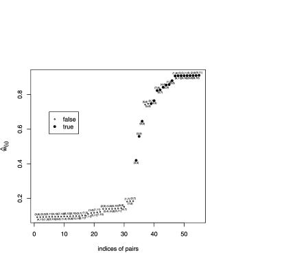
Figure 2: Posterior means $\hat{w}_{(i,j)}$ of $(w_{ij}+w_{ji})/2$, sorted in increasing order, from one MCMC run of the HM on the simulated data with constant intrinsic variances. Large solid and small empty circles represent true and false associations, respectively.

To infer the pair of proteins that are associated, we need to set a threshold $u_{1}$ on the posterior means $\hat{w}_{(i,j)}$ so that those above the threshold are inferred to be associated. The permutation study offers an over-liberal threshold ($<$0.1), based on which we get over 40 associations with false positive rate $\geq$0.5. Noting the jumps in the plot of $\hat{w}_{(i,j)}$, we propose to choose the threshold where a big jump occurs. Setting the threshold $u_{1}$ as any value between 0.2 and 0.4 and choosing the pairs with $\hat{w}_{(i,j)}>u_{1}$, we get 22 associations with 2 false positives. When we have multiple MCMC runs, which lead to multiple plots of $\hat{w}_{(i,j)}$, we can combine the inferences from them. Figure S1 in the Supplementary Material [Luo and Zhao (2010)] draws the plots of $\hat{w}_{(i,j)}$ from four additional MCMC runs. They show the same features as seen in Figure 2 that true associations tend to have high $\hat{w}_{(i,j)}$ values and jumps exist in these plots. These five MCMC runs lead to quite similar results: from four of them we get 22 associations with 2 false positives, and from a fifth run we get 21 associations with 2 false positives and 1 missing association, when we choose $u_{1}$ between 0.3 and 0.4. Let $u_{f}$ be the relative frequency that each association is selected. When $u_{1}\in(0.3,0.4)$ and $u_{f}\geq 4/5$, we get 22 associations with 2 false positives (Figure 3).

Figure 3: Networks inferred by choosing associations with $u_{1}\in(0.3,0.4)$, $u_{2}=0.1$, $u_{3}\in(0.3,0.5)$, and $u_{f}\geq 0.8$ in five MCMC runs of the HM on the simulated data with constant $\sigma_{i}^{I}$. Solid arrowed lines represent correctly inferred true edges, dashed thick lines with labels “u” represent edges whose directions cannot be determined from the simulations, dashed arrowed thin lines with labels “r” represent reversed edges, and dotted lines with labels “+” represent false positive edges.

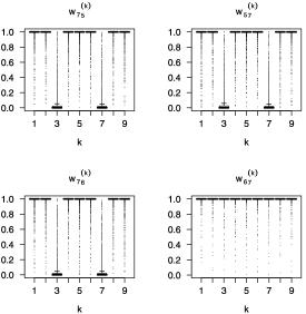
Figure 4: Boxplots of the samples from the posterior distributions of $w^{(k)}_{57}$ and $w^{(k)}_{75}$ (top panel), $w^{(k)}_{67}$ and $w^{(k)}_{76}$ (bottom panel) when $v_{ij}\equiv 0.1$ for all $i$ and $j$. This is from one MCMC run of the HM on the simulated data with constant $\sigma_{i}^{I}$.

For the pairs of proteins that are inferred to be associated, we then infer their causal directions based on the criteria listed in Section 2.1. To better illustrate the criteria, we give two examples in Figure 4. The top panel draws the boxplots of the samples from the posterior distributions of $w^{(k)}_{57}$ and $w^{(k)}_{75}$. Both show that the experimental-level probabilities greatly decreased under conditions 3 and 7 where protein 7 (Akt) is inhibited (here $\max_{k}\{\hat{w}^{(k)}_{57}\}-\hat{w}^{(k^{\prime})}_{57}\geq 0.8$ and $\max_{k}\{\hat{w}^{(k)}_{75}\}-\hat{w}^{(k^{\prime})}_{75}=0.9$ for $k^{\prime}=3,7$). So we infer the direction $5\rightarrow 7$ (i.e., PIP3 $\rightarrow$ Akt). The bottom panel tells a different story. The posterior means of $w^{(k)}_{76}$ when $k=3$ or 7 are much smaller than others ($\max_{k}\{\hat{w}^{(k)}_{76}\}-\hat{w}^{(k^{\prime})}_{76}=0.9$), indicating the causal relation $6\rightarrow 7$, but $w^{(k)}_{67}$ keeps the same level under all conditions ($\max_{k}\{\hat{w}^{(k)}_{67}\}-\hat{w}^{(k^{\prime})}_{67}=0$), indicating the causal relation $7\rightarrow 6$. The contradictory results from $w^{(k)}_{67}$ and $w^{(k)}_{76}$ lead to the failure in determining the causal relationship between proteins 6 (Erk) and 7. Taking $u_{2}=0.1$ and $u_{3}\in(0.3,0.5)$, we infer a causal network as shown in Figure 3, which contains 14 true directed edges, 5 edges whose directions are undetermined, 1 reversed edge, and 2 false edges.

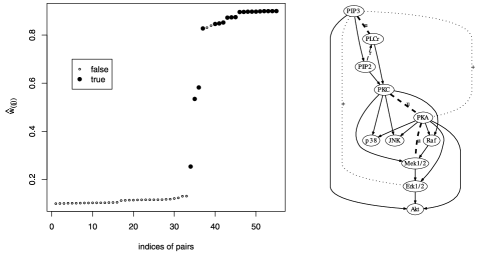
Figure 5: Inference from RHM with $v_{ij}=0.1$ on the simulated data with constant $\sigma_{i}^{I}$. Left: posterior means $\hat{w}_{(i,j)}$ of $w_{ij}$, sorted in increasing order. Right: inferred networks with $u_{1}^{\prime}=0.2$, $u_{3}\in(0.3,0.5)$. Solid arrowed lines represent correctly inferred true edges, dashed thick lines with labels “u” represent edges whose directions cannot be determined from the simulations, dashed arrowed thin lines with labels “r” represent reversed edges, and dotted lines with labels “+” represent false positive edges.

When we have multiple MCMC runs, we infer the causal relation of each edge based on the majority vote of the directions inferred from each MCMC run. In fact, these five runs lead to almost identical causal inference for the common associations [based on $u_{1}\in(0.3,0.4)$] when we take $u_{2}=0.1$ and $u_{3}\in(0.3,0.5)$. The choices of $u_{2}$ and $u_{3}$ are affected by the value of $v_{ij}^{(k)}$. Choosing $v_{ij}^{(k)}\equiv 0.1$ ensures that most $\hat{w}_{ij}^{(k)}$ are either above 0.9 or below 0.1. The streams with $\hat{w}_{ij}^{(k)}\leq 0.1$ for all $k$ contain too weak a signal to provide sufficient information for causal inference. So we take $u_{2}=0.1$. The small value of $v_{ij}^{(k)}$ also leads to a great difference in $\hat{w}_{ij}^{(k)}$ for different experiments when protein $i$ or $j$ is intervened. In this simulation study, intervention of the child node for one edge leads to a decrease of at least 0.5 in $\hat{w}_{ij}^{(k)}$. Any value of $u_{3}$ in (0.3, 0.5) leads to the same directional inference for the inferred associations.

3.1.2 Inference from RHM

RHM requires that $w_{ij}=w_{ji}$ and $w^{(k)}_{ij}=w^{(k)}_{ji}$ for all $i$, $j$, and $k$. This restriction aims at avoiding the nonconsistent directional inferences based on $w^{(k)}_{ji}$ and $w^{(k)}_{ij}$ separately as HM does. We plot the posterior means $\hat{w}_{(i,j)}$ of $w_{ij}$ in Figure 5 where we take $v_{ij}=0.1$. Similar to Figures 2 and S1, true associations tend to have higher values of $\hat{w}_{(ij)}$. Setting $u^{\prime}_{1}=0.2$, we infer 22 associations with 2 false positives. Applying the criteria listed in Supplementary Material S3 [Luo and Zhao (2010)], we infer the causal network as shown in Figure 5. Compared to the network in Figure 3, RHM leads to a network with 16 true directed edges, 3 edges whose directions are undetermined, 1 reversed edge, and 2 false edges when we take $u^{\prime}_{1}=0.2$ and $u_{3}\in(0.3,0.5)$. If we increase the threshold $u^{\prime}_{1}$ to a value where there is a big jump, for example, 0.3, we will miss 1 true directed edge.

When a bigger value $v_{ij}=10$ is applied, the differences of the posterior means $\hat{w}_{(i,j)}$ of $w_{ij}$ become much smaller between the true and false associations (Figure S2 in the Supplementary Material [Luo and Zhao (2010)]). This together with the fact that bigger values of $v_{ij}$ lead to smaller changes in experimental level probabilities results in our conclusion that a small $v_{ij}$ is preferred for causal network inference.

3.1.3 Inference from NHM

Ignoring the effect of perturbations on signaling pathway, NHM assumes a common coefficient $\alpha_{ij}$ in the linear regression models across all experimental conditions. From this model, we can only infer whether there is an association between two proteins. Similar to the inferred posterior means from HM, $\hat{w}_{(i,j)}$ from NHM also tend to take higher values for true associations (Figure 6), but with two differences. First, the range of $\hat{w}_{(i,j)}$ from NHM is smaller. In other words, compared to HM, NHM leads to smaller values of the biggest $\hat{w}_{(i,j)}$, and larger values of the smallest $\hat{w}_{(i,j)}$. So the support for true associations and the evidence against false associations are weaker. Second, the dominance of high values of true associations is not as strong as that from HM. More false associations take higher values of $\hat{w}_{(i,j)}$ than the hierarchical inference. If we take 0.6 as a threshold, we infer 23 associations with 15 true and 8 false. Taking 0.45 as the threshold, we recover all the true associations, but 27 false ones are also inferred. More importantly, we cannot determine the directions of associations from NHM because perturbation information is not utilized in this model.

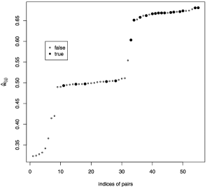
Figure 6: Posterior means $\hat{w}_{(i,j)}$ of $(w_{ij}+w_{ji})/2$, sorted in increasing order, from one MCMC run of NHM. Small empty and large solid circles represent the false and true associations, respectively.

3.2 Variable intrinsic variances $(\sigma^{I}_{i})^{2}$

We then consider the case where variances of intrinsic noises vary for different proteins. In this case, both HM and RHM with $v_{ij}=0.1$ clearly separate the true associations from the false ones in the plot of the posterior means $\hat{w}_{(i,j)}$ (Figure 7). The causal networks inferred from both models are the same, with 18 correctly inferred true edges, 1 reversed edge, and 1 edge whose direction is undetermined [$u_{1}\in(0.2,0.7)$, $u_{2}=0.1,$ and $u_{3}=0.3$]. As in Section 3.1.2, RHM with a bigger value $v_{ij}=10$ leads to association inference with bigger false positive rate and smaller changes in experimental level probabilities when a child node is perturbed (Figure S2 in the Supplementary Material [Luo and Zhao (2010)]). NHM is not applied here and thereafter since it does not provide causal relations.

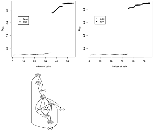
Figure 7: Inference results for the simulated data with variable intrinsic variances. Upper panel: posterior means $\hat{w}_{(i,j)}$ of $w_{ij}$, sorted in increasing order from HM (left) and RHM with $v_{ij}=0.1$ (right). Lower panel: inferred networks from both models with $u_{1}\in(0.2,0.7)$ and $u_{3}=0.3$. Solid arrowed lines represent correctly inferred true edges, dashed thick lines with labels “u” represent edges whose directions cannot be determined from the simulations, and dashed arrowed thin lines with labels “r” represent reversed edges.

Table 2: Summary of pathway inference in simulation study

Data	Methods	True	Undetermined	Reversed	Missing	False	Hamming
							distance
Data-1	HM	14	5	1	0	2	08
	RHM	16	3	0	1	2	06
Data-2	HM	18	1	1	0	0	02
	RHM	18	1	1	0	0	02
Data-$1^{t}$	HM	09	4	1	6	4	15
Data-$2^{t}$	HM	14	1	0	5	6	12

[]All are based on $u_{1}=0.4$ and $u_{3}=0.3$. The hamming distance is the minimum number of simple operations needed to go from the inferred graph to the true graph. Here simple operations include adding or removing an edge, and adding, removing, or changing the direction of an edge. Data-1: simulated data in Section 3.1 with constant intrinsic variances. Data-2: simulated data in Section 3.2 with varying intrinsic variances. Data-$1^{t}$: simulated data with parameter settings in Data-1 and intrinsic noises sampled from $t(1)$. Data-$2^{t}$: simulated data with parameter settings in Data-2 and intrinsic noises sampled from $t(1)$.

3.3 Heavy tail distribution for intrinsic noise

Considering the possibility of nonnormality for real biological processes, we simulate data where the expression levels of proteins have heavy tail distribution. This is realized by simulating $\varepsilon_{\mathit{ink}}^{I}\sim\mathrm{t}(1)$ for each protein $i$ under each experimental condition $k$. We reuse the parameter settings in Sections 3.1 and 3.2 so that the performance of our methods on the normal and nonnormal cases can be easily compared. We summarize the network inference results in Table 2. Due to the model misspecification when we use HM to analyze these heavy tail distributed data, we infer networks with more false positive and false negative edges. Therefore, our current model needs to be extended to analyze heavy tail data.

4 Case study

The Mitogen-Activated Protein Kinase (MAPK) pathways transduce a large variety of external signals, leading to a wide range of cellular responses such as growth, differentiation, inflammation, and apoptosis. External stimuli are sensed by cell surface markers, then travel through a cascade of protein modifications of signaling proteins, and eventually lead to changes in nuclear transcription. Single cell interventional data of 11 well-studied proteins from the MAPK pathways were originally generated by Sachs et al. (2005) using the intracellular multicolor flow cytometry technique. This pathway was perturbed by 9 different stimuli, each targeting a different protein in the selected pathway (Figure 1 and Table 1). Sachs et al. (2005) applied Bayesian network analysis to infer the causal protein-signaling network. Correcting the bias in the commonly used algorithm proposed by Friedman and Killer (2003), Ellis and Wong (2008) reanalyzed this data set through sampling BN structures from the correct posterior distribution. Both studies used the discretized data where the protein expression levels were grouped into three levels: “low,” “middle,” and “high.” The inhibited molecules were set at “low” values, and activated molecules were set to level “high.” We apply our method to this data and compare the results with those from Ellis and Wong (2008).

We infer the networks using HM and RHM with $v_{ij}=0.1$ and $v_{ij}=10$. Each analysis has five MCMC runs. Figure 8 shows the inferred posterior means $\hat{w}_{(i,j)}$ in one MCMC run (more can be found in Supplementary Figures S4 $\sim$ S6 [Luo and Zhao (2010)]), and the inferred networks from five MCMC runs, from each method. We use the same symbols as in simulation studies to indicate true or false inferences, where the “true” network is taken to be the network in Figure 3 of Sachs et al. (2005), which is the current understanding of this pathway.

Compared to HM, RHMs lead to fewer true associations with high values of $\hat{w}_{(i,j)}$ ($v_{ij}=10$) or smaller gaps of $\hat{w}_{(i,j)}$ between most true and false associations ($v_{ij}=0.1$). Taking the threshold $u_{1}=0.2$ and requiring $u_{f}\geq 0.6$ in five runs of HM, we get 21 associations, with 5 missing edges and 6 false positives. Requiring $u^{\prime}_{1}=0.11$ and $u_{f}\geq 0.6$ in RHM with $v_{ij}=0.1$, we get 19 associations, with 5 missing edges and 4 false ones. The threshold 0.11 exceeds the value (0.1) from the permutation study by only a small amount, implying that RHM offers weaker support to true associations than HM. Setting $u^{\prime}_{1}=0.994$ and $u_{f}\geq 0.6$ in RHM with $v_{ij}=10$, we only get 14 associations, with 8 missing and 2 false associations.

Figure 8: Inference results for the real data. From top to bottom: HM, RHM with $v_{ij}=0.1$, and RHM with $v_{ij}=10$. In networks, solid arrowed lines represent correctly inferred true edges, dashed thick lines with labels “u” represent edges whose directions cannot be determined from the simulations, dashed arrowed thin lines with labels “r” represent reversed edges, dotted arrowed thick lines represent missing edges, and dotted thin lines with labels “+” represent false positive edges.

Table 3: Summary of the inferred networks applying different methods to the real data

	True	Undetermined	Reversed	Missing	False	Hamming distance
HM	9	1	4	6	4	15
RHM $v_{ij}=0.1$	6	8	1	5	4	18
RHM $v_{ij}=10$	5	5	2	8	2	17
mHM	6	5	1	8	4	18
BN	9	0	3	8	6	17

[]Here mHM denotes the modified model described in Supplementary Material S1 [Luo and Zhao (2010)] which models the varying variances of intrinsic noises.

From RHM, we can only correctly infer the directions of five or six edges. The causal relations for most inferred associations can not be determined. But HM leads to a better result: 9 true directed edges, 1 direction-undetermined, 4 reversed, 6 missed, and 4 false edges, under the thresholds $u_{1}=0.2$, $u_{2}=0.1$, $u_{3}=0.3$, and $u_{f}\geq 0.8$ (Figure 8 and Table 3). This inferred network is comparable with that from Ellis and Wong (2008), which contains 9 true directed edges, 3 reversed, 8 missed, and 6 false edges. The Hamming distances of these two networks to Figure 1 are 15 and 17, respectively. These results are summarized in Table 3.

In MCMC analysis, we take $\beta_{i}=\gamma_{j}=1$ for $i=1,2$ and $j=1,\ldots,6$. To check the sensitivity of HM, we also consider other values: $\gamma_{i}=0.1$ or 100, and $\beta_{j}=0.1$ or 0.0001. Taking $\beta_{j}=0.1$, we get a network (not shown) with 9 true directed edges, 1 direction-undetermined, 4 reversed, 6 missed, and 6 false associations. Other values of the hyperparameters result in 1$\sim$3 fewer true associations, and at least 3 fewer true directed edges. All these results are based on 5,500,000 iterations of MCMC updates in each run, which take about 20 hours on a node with an Intel(R) Xeon(R) 3 GHz CPU and a 16G memory.

5 Discussion

We have proposed hierarchical statistical methods to infer a signaling pathway from single cell data collected from a set of perturbation experiments. The advantage of this method is that it provides a more explicit framework to relate the activity levels of different proteins. In our models, we assume that the activity level of each protein is linearly associated with a small subset of other proteins under each condition. Using a Bayesian hierarchical structure, we model the existence of an association between two proteins both at the overall level and at the experimental level. The overall-level probabilities measure the strength of associations between any two proteins across all experiments. The experimental-level probabilities reflect the changes of associations between proteins under different conditions. Our inferential procedure consists of two steps. First we infer the existence of an association between any pair of proteins based on the overall-level probabilities. Then for those pairs of proteins inferred to be associated, we infer the directions of the causal relations based on the changes in the experimental level probabilities. The basic rationale in our causal inference is that for two associated proteins, controlling over the target molecule destroys the association, while perturbing the regulatory molecule does not.

We consider hierarchical models with (RHM) and without (HM) the restriction that $w_{ij}=w_{ji}$ and $w_{ij}^{(k)}=w_{ji}^{(k)}$ for each $k$. For RHM, we have to specify the hyperparameter $v_{ij}$ prior to MCMC analysis. We have considered the inference results when the value of $v_{ij}$ is set at 0.1 and 10. Higher values of $v_{ij}$ lead to higher ranges of the inferred overall-level and experimental-level probabilities, and smaller changes in experimental-level probabilities. In HM, the experimental-level probabilities can be integrated out, so the posterior inference of other parameters is independent of $v_{ij}$. Hence, the choice of associations, which is based on the overall-level probabilities, is independent of $v_{ij}$. We only need to specify $v_{ij}$ in the causal inference. To better reflect the changes of the experimental-level probabilities, we suggest smaller values for $v_{ij}$, for example, $v_{ij}=0.1$. Both HM and RHM perform well in simulation studies.

We need to choose thresholds to infer the causal network: $u_{1}$ for association inference and $u_{2}$ and $u_{3}$ for causal directional inference. Noting the jumps in the plots of $\hat{w}_{(ij)}$, we propose to choose the threshold $u_{1}$ where there are great differences in sorted $\hat{w}_{(ij)}$. This is easily determined when variations in the data are well captured by the proposed hierarchical models (e.g., Figures 2 and 7). If there are no great differences in the sorted overall-level probabilities (e.g., Figure 8), one may decide the number of edges to be included and then choose the top ones. Threshold $u_{2}$, which is taken as 0.1 in our study, can be chosen based on the experimental-level probabilities of those unassociated pairs of proteins. Threshold $u_{3}$ is closely related to $v_{ij}$, which measures the variability in $\hat{w}_{ij}^{(k)}$ in that a smaller $v_{ij}$ leads to greater variabilities in $\hat{w}_{ij}^{(k)}$ between the experiments when the target protein is and is not intervened. When $v_{ij}=0.1$, a difference of 0.3 in $\hat{w}_{ij}^{(k)}$ is enough to show the effect of intervening the target protein.

Compared to the nonhierarchical model, hierarchical models have at least two advantages. First, the hierarchical structure allows information borrowing across different experiments while allowing for differences among experiments, leading to a more clear-cut inference on whether two proteins are related. Second, this modeling framework allows us to infer causal relationships between proteins from the presence and absence of the association across different perturbation conditions. Overall, our proposed hierarchical modeling provides a general framework for inferring networks from high-throughout data.

There are several possible ways of extending this model. In Supplementary Material S1 [Luo and Zhao (2010)] we modify HM by incorporating varying variances of intrinsic noises under different experimental conditions. The modified model does not outperform HM in our simulation study. It is interesting to investigate when the varying variances of intrinsic noises are not ignorable and incorporating them improves the network inference. We also find in our simulation study that applying our methods to data where intrinsic noises are sampled from heavy tail distributions results in power loss in pathway inference. Therefore, there is a need to extend this hierarchical structure to model nonnormal data.

Additional descriptions and results of hierarchical models
[doi]10.1214/10-AOAS425SUPP [url]http://lib.stat.cmu.edu/aoas/425/supplement.pdf .pdf Materials include description and simulation results of the hierarchical model (mHM) with varying variances of intrinsic noises $(\sigma_{ik}^{I})^{2}$, MCMC algorithm for the hierarchical model (HM), direction inference for the restricted hierarchical model (RHM), and additional figures of posterior inference and networks.

References

- Dobra et al. (2004) Dobra, A., Hans, C., Jones, B., Nevins, J., Yao, G. and West, M. (2004). Sparse graphical models for exploring gene expression data. J. Multivariate Anal. 90 196–212. \MR2064941
- Ellis and Wong (2008) Ellis, B. and Wong, W. H. (2008). Learning causal Bayesian network structures from experimental data. J. Amer. Statist. Assoc. 103 778–789. \MR2524009
- Friedman and Killer (2003) Friedman, N. and Killer, D. (2003). Being Bayesian about network structure. Machine Learning 50 95–126.
- Heckerman et al. (2000) Heckerman, D., Chickering, D. M., Meek, C., Rounthwaite, R. and Kadie, C. (2000). Dependency networks for inference, collaborative filtering, and data visulization. J. Mach. Learn. Res. 1 49–75.
- Herzenberg et al. (2002) Herzenberg, L. A., Parks, D., Sahaf, B., Perez, O., Roederer, M. and Herzenberg, L. A. (2002). The history and future of the fluorescence activated cell sorter and flow cytometry: A view from Stanford. Clinical Chemistry 48 1819–1827.
- Lauritzen (1996) Lauritzen, S. L. (1996). Graphical Models. Clarendon Press, Oxford. \MR1419991
- Liu and Ringnér (2007) Liu, Y. and Ringnér, M. (2007). Revealing signaling pathway deregulation by using gene expression signatures and regulatory motif analysis. Genome Biology 8 R77.1–R77.10.
- Luo and Zhao (2010) Luo, R. and Zhao, H. (2010). Supplementary material for “Bayesian hierarchical modeling for signaling pathway inference from single cell interventional data.” DOI: 10.1214/10-AOAS425SUPP.
- Pe’er (2005) Pe’er, D. (2005). Bayesian network analysis of signaling networks: A primer. Science’s STKE 281 1–12.
- Pe’er et al. (2001) Pe’er, D., Regev, A., Elidan, G. and Friedman, N. (2001). Inferring subnetworks from perturbed expression profiles. Bioinformatics 17 Suppl. S215–S224.
- Perez and Nolan (2002) Perez, O. D. and Nolan, G. (2002). Simultaneous measurement of multiple active kinase states using polychromatic flow cytometry. Nature Biotechnology 20 155–162.
- Sachs et al. (2005) Sachs, K., Perez, O., Pe‘er, D., Lauffenburger, D. A. and Nolan, G. P. (2005). Causal protein-signaling networks derived from multiparameter single-cell data. Science 308 523–529.
- Schäfer and Strimmer (2005) Schäfer, J. and Strimmer, K. (2005). An empirical Bayes approach to inferring large-scale gene association networks. Bioinformatics 21 754–764.
- Wei and Li (2007) Wei, W. and Li, H. (2007). A Markov random field model for network-based analysis of genomic data. Bioinformatics 23 1537–1544.
- Wei and Li (2008) Wei, W. and Li, H. (2008). A hidden spatial–temporal Markov random field model for network-based analysis of time course gene expression data. Ann. Appl. Statist. 2 408–429. \MR2415609
- Werhli, Grzegorczyk and Husmeier (2006) Werhli, A. V., Grzegorczyk, M. and Husmeier, D. (2006). Comparative evaluation of reverse engineering gene regulatory networks with relevance networks, graphical Gaussian models and Bayesian networks. Systems Biology 22 2523–2531.