Spectrum of Radiation from Rough Surfaces

Abstract

Radiation from a charged particle travelling parallel to a rough surface has been considered. Spectral-angular intensity is calculated in the weak scattering regime. It is shown that the main contribution to the radiation intensity is determined by the multiple scattering of polaritons induced by a charge on the surface. Multiple scattering effects lead to strong frequency dependence of radiation intensity. Possible applications in beam and surface diagnostics are discussed.

1 Introduction

Light scattering from rough surfaces attracted much interest [1]. In particular this interest is caused by the determination of microtopographic properties of rough metallic surfaces from the light scattering measurements [2]. The enhancement of intensity of scattered light on a rough surface is due to a resonant excitation of surface polaritons induced by incident light. Surface polaritons are multiply scattered on the roughness resulting in their diffusion and localisation[3] that lead to peculiarities in the light scattering from rough surfaces.

Polaritons can be induced not only by an incident light but also by a charged particle. It is interesting to reveal the manifestation of polaritons multiple scattering on the charged particle radiation from rough surfaces. Origination of this radiation is due to the scattering of polaritons induced by the charged particle on the inhomogeneites of dielectric constant associated with the roughness of the surface. Earlier in this geometry main attention was paid to the periodical grating case when Smith-Purcell radiation(SPR) [4] is originated. Recently we have considered [5] the radiation from an uncorrelated rough surface.

In the present paper we consider the influence of multiple scattering effects, including the localisation of polaritons, on the radiation of a charged particle travelling over a correlated rough surface.We will see that they lead to strong frequency dependence of intensity. Strong frequency dependence allows to separate the diffusional mechanism of radiation from other radiation mechanisms.

2 Formulation of the Problem

A charged particle moves uniformly in the vacuum at the distance $d$ from the plane $z=0$ separating vacuum and the isotropic medium distorted by roughness. We are interested in radiation field far away from the charge and interface. Maxwell equation for the electric field has the form

$$\nabla^{2}\vec{E}(\vec{r},\omega)-\rm{grad}div\vec{E}(\vec{r},\omega)+\frac{\omega^{2}}{c^{2}}\varepsilon(\vec{r},\omega)\vec{E}(\vec{r},\omega)=\vec{j}(\vec{r},\omega)$$ (1)

where $\vec{j}(\vec{r},\omega)=-\frac{4\pi ie\omega\vec{v}}{vc^{2}}\delta(z-d)\delta(y)e^{i\omega x/v}$ is the current density associated with the charge. Here $\vec{v}$ is the velocity of the particle moving on $0x$ direction and $\varepsilon(\vec{r},\omega)$ is the inhomogeneous dielectric permittivity of the system. For a rough surface it can be chosen as $\varepsilon(\vec{r},\omega)=\varepsilon_{0}(z,\omega)+\varepsilon_{r}(\vec{r},\omega)$, where $\varepsilon_{0}(z,\omega)=\Theta(z)+\Theta(-z)\varepsilon(\omega)$ descibes the flat interface vacuum-metal and $\varepsilon_{r}(\vec{r},\omega)=[\varepsilon(\omega)-1]\delta(z)h(x,y)$ is the contribution of small roughness. $h(x,y)$ is the amplitude of surface roughness. To separate the radiation field one should decompose the electric field as $\vec{E}=\vec{E}_{0}+\vec{E}_{r}$, analogous to the decomposition of dielectric constant. $\vec{E}_{0}$ and $\vec{E}_{r}$ are the background field created by the charge and the radiation field,respectively. They obey the following equations

$$\nabla^{2}\vec{E}_{0}(\vec{r},\omega)-\rm{grad}div\vec{E}_{0}(\vec{r},\omega)+$$

$$+\frac{\omega^{2}}{c^{2}}\varepsilon_{0}(z,\omega)\vec{E}_{0}(\vec{r},\omega)=\vec{j}(\vec{r},\omega)$$ (2)

$$\nabla^{2}\vec{E}_{r}(\vec{r},\omega)-\rm{grad}div\vec{E}_{r}(\vec{r},\omega)+\frac{\omega^{2}}{c^{2}}\varepsilon(z,\omega)\vec{E}_{r}(\vec{r},\omega)+$$

$$+\frac{\omega^{2}}{c^{2}}\varepsilon_{r}(\vec{r},\omega)\vec{E}_{r}(\vec{r},\omega)=-\frac{\omega^{2}}{c^{2}}\varepsilon_{r}(\vec{r},\omega)\vec{E}_{0}(\vec{r},\omega)$$ (3)

Radiation intensity at the frequencies $\omega$, $\omega+d\omega$ and at the angles $\Omega$, $\Omega+d\Omega$ is determined as $dI(\omega,\vec{n})=\frac{c}{2}|\vec{E}_{r}(\vec{R})|^{2}R^{2}d\Omega d\omega$, where $\vec{n}$ is unit vector on the direction of observation point $\vec{R}$, $\Omega$ is the corresponding solid angle, see [5]. Radiation intensity should be averaged over the realizations of random roughness $h(x,y)$. For this reason it is convenient to introduce the Green’s functions of Eqs.(2,3). One can represent the averaged radiation intensity tensor $<I_{ij}(\vec{R})>=<E_{ri}(\vec{R})E^{*}_{rj}(\vec{R})>$ in the form

$$<I_{ij}(\vec{R})>=\frac{\omega^{4}}{c^{4}}\int d\vec{r}d\vec{r}^{\prime}<G_{i\mu}(\vec{R},\vec{r})\varepsilon_{r}(\vec{r})$$

$$G_{\nu j}^{*}(\vec{r}^{\prime},\vec{R})\varepsilon_{r}(\vec{r}^{\prime})>E_{0\mu}(\vec{r})E_{0\nu}^{*}(\vec{r}^{\prime})$$ (4)

where the background electric field $E_{0\mu}(\vec{r})=\int d\vec{r}_{1}G^{0}_{\mu\lambda}(\vec{r},\vec{r}_{1})j_{\lambda}(\vec{r}_{1})$ is expressed through the bare Green’s function. Here $<...>$ means an averaging over the surface random profile $h(x,y)$. Note that in the original Smith-Purcell experiment [4] as well as in subsequent works on SPR mainly a periodical grating in one direction is used. In this case $h(x,y)\equiv h(x)$ is a some periodical function of one coordinate. In the present paper we consider correlated random grating case. We suppose that $h$ is a gaussian stochastic process characterized by two parameters $<h(\vec{\rho})>=0,<h(\vec{\rho}_{1})h(\vec{\rho}_{2})>=\delta^{2}W_{0}(|\vec{\rho}_{1}-\vec{\rho}_{2}|)$, where $\vec{\rho}$ ia a two dimensional vector in the $xy$ plane, $\delta^{2}=<h^{2}(\vec{\rho})>$ is the average deviation of surface from the plane $z=0$. Correlation function $W_{0}$ is characterized by a correlation length $\sigma$ at which it is essentially decreased. Maxwell equations for electric fields Eq.(2,3) and Green’s functions should be amended by the boundary conditions. As usual, it is required that tangential components of electric field be continues across the plane $z=0$. The exact field, of course, will satisfy the boundary conditions across the surface $z=h(x,y)$ rather than the plane. However this approximation seems reasonable for small roughness $\lambda\gg\delta$ and is widely used in literature. The Green’s function $G_{\mu\nu}(\vec{r},\vec{r}^{\prime},\omega)$, when considered a function of $z$ for fixed $z^{\prime}$ satisfies the same boundary condition as the $\mu th$ Cartesian component of electric field.

3 Green’s Functions

The equation for bare Green’s function with the correct boundary conditions for arbitrary $\varepsilon(\omega)$ was solved in [6]. To obtain radiation intensity in vacuum we will need Green’s functions in the half space $z>0$. In order to simplify the problem we will consider the case when isotropic medium is a metal with very large negative dielectric constant $|\varepsilon(\omega)|\gg 1$. In the limit $|\varepsilon|\to\infty$ the following components survive [6]

$$G_{zz}^{0}(\vec{p}|0,z)=G_{zz}^{0}(\vec{p}|z,0)=\frac{ip^{2}}{k^{2}}\frac{\varepsilon(\omega)e^{iqz}}{k_{1}-\varepsilon(\omega)q}$$

$$G_{xz}^{0}(\vec{p}|0,z)=-G_{zx}^{0}(\vec{p}|z,0)=-\frac{ip_{x}}{k^{2}}\frac{\varepsilon(\omega)qe^{iqz}}{k_{1}-\varepsilon(\omega)q}$$ (5)

where $G_{ij}^{0}(\vec{p}|z,z^{\prime})$ is the two-dimensional Fourier transform of $G_{ij}^{0}(\vec{r},\vec{r}^{\prime})$ and $z>0$. Here $\vec{p}$ and $\vec{\rho}$ are two-dimensional vectors with Cartesian components $p_{x},p_{y},0$ and $x,y,0$. Also $k=\omega/c$, $k_{1}$ and $q$ are determined as follows:

$$q=\left\{\sqrt{k^{2}-p^{2}},\quad k^{2}>p^{2}\atop i\sqrt{p^{2}-k^{2}},\quad k^{2}<p^{2}\right.$$ (6)

$$k_{1}=-(\varepsilon(\omega)k^{2}-p^{2})^{1/2}$$ (7)

A branch cut for the square root in Eq.(7) along the negative real axis is assumed [6]. Other components of Green’s function are small for large $|\varepsilon|$. To determine radiation intensity we will need asymptotics of Green’s functions at large distances. Using Eq.(5) and making a Fourier transform, one finds [5]

$$G_{zz}^{0}(\vec{R},\vec{\rho},0)\approx\frac{1}{2\pi\sqrt{2}R}\left[n_{z}\sqrt{n_{\rho}}\cos\left(k(R-\vec{n}_{\rho}\vec{\rho})-\frac{\pi}{4}\right)+\right.$$

$$\left.+\frac{n_{z}}{\sqrt{n_{\rho}}}\cos\left(k(R-\vec{n}_{\rho}\vec{\rho})+\frac{\pi}{4}\right)\right]+$$

$$+\frac{i}{2\pi\sqrt{2}R}\left[\sqrt{n_{\rho}}\cos\left(k(R-\vec{n}_{\rho}\vec{\rho})+\frac{\pi}{4}\right)-\right.$$

$$\left.-\frac{1}{\sqrt{n_{\rho}}}\cos\left(k(R-\vec{n}_{\rho}\vec{\rho})-\frac{\pi}{4}\right)\right];$$

$$G_{xz}^{0}(\vec{R},\vec{\rho},0)=-G_{zx}^{0}(\vec{\rho},0,\vec{R})\approx$$

$$\approx\frac{1}{2\pi\sqrt{2}R}\left[n_{x}\sqrt{n_{\rho}}\sin\left(k(R-\vec{n}_{\rho}\vec{\rho})+\frac{\pi}{4}\right)+\right.$$

$$\left.+\frac{n_{x}}{\sqrt{n_{\rho}}}\sin\left(k(R-\vec{n}_{\rho}\vec{\rho})-\frac{\pi}{4}\right)\right]+$$

$$+\frac{i}{2\pi\sqrt{2}R}\left[\sqrt{n_{\rho}}n_{x}n_{z}\sin\left(k(R-\vec{n}_{\rho}\vec{\rho})-\frac{\pi}{4}\right)-\right.$$

$$\left.-\frac{n_{z}n_{x}}{\sqrt{n_{\rho}}}\sin\left(k(R-\vec{n}_{\rho}\vec{\rho})+\frac{\pi}{4}\right)\right]$$ (8)

where $\vec{n}$ is the unit vector on the direction of the observation point $\vec{R}=\vec{n}R$, $n_{x,z}$ and $n_{\rho}$ are it’s corresponding components. Eqs.(8) are correct provided that $kR\gg 1$, $R_{\rho}\gg\rho$ and we use approximate equation $|\vec{R}-\vec{r}|\approx R-\vec{n}\vec{r}$.

4 Radiation Intensity

Spectral-angular radiation intensity Eq.(4) can be represented as a sum of three contributions, $I(\vec{R},\omega)=I^{0}(\vec{R},\omega)+I^{D}(\vec{R},\omega)+I^{C}(\vec{R},\omega)$, where $I^{0}$ , $I^{D}$ and $I^{C}$ are single scattering , diffusive and maximally crossed diagram contributions, respectively [7, 8, 9]. First consider the single scattering contribution to the radiation intensity. Substituting the Green’s functions in Eq.(4) by the bare ones, we obtain

$$I_{ij}^{0}(\vec{R})=\int d\vec{\rho}d\vec{\rho}^{\prime}G^{0}_{iz}(\vec{R},\vec{\rho},0)G^{*0}_{zj}(\vec{\rho}^{\prime},0,\vec{R})$$

$$W(|\vec{\rho}-\vec{\rho}^{\prime}|)E_{0z}(\vec{\rho},0)E^{*}_{0z}(\vec{\rho}^{\prime},0)$$ (9)

where $(ij)\equiv(xz)$ and $W(\rho)\equiv(\varepsilon-1)^{2}k^{4}\delta^{2}W_{0}(\rho)$.

The background electric field in the limit $|\varepsilon|\to\infty$ can be found from Eq. (5) and the form of the current density

$$E_{0z}(\vec{\rho},0)=-\frac{4ee^{ik_{0}x}}{v}\frac{dk_{0}}{\gamma\sqrt{y^{2}+d^{2}}}K_{1}(\frac{k_{0}\sqrt{y^{2}+d^{2}}}{\gamma})$$ (10)

where $k_{0}=\omega/v$, $\gamma=(1-v^{2}/c^{2})^{-1/2}$ is the Lorentz factor of the particle and $K_{1}$ is the first order Macdonald function. As follows from Eq.(10) the background electric field and correspondingly radiation intensity is exponentially small when $k_{0}d/\gamma\gg 1$. An essential intensity exists for $k_{0}d/\gamma\ll 1$. Far away from the system at the observation point one can use asymptotic expressions for Green’s functions Eq.(8). Substituting Eqs.(8) into Eq.(9), for the spectral-angular radiation intensity $I(\omega,\Omega)=cR^{2}I_{ii}(\vec{R})/2$, one obtains

$$I^{0}(\omega,\Omega)=\frac{c}{32\pi^{2}}\frac{(1+n_{\rho}^{2})(1+n_{z}^{2})(1-n_{x}^{2})}{n_{\rho}}\times$$

$$\times\int dxdx^{\prime}dydy^{\prime}\cos[k\vec{n}_{\rho}(\vec{\rho}-\vec{\rho}^{\prime})]W(|(\vec{\rho}-\vec{\rho}^{\prime})|)\times$$

$$\times E_{0z}(\vec{\rho},0)E^{*}_{0z}(\vec{\rho}^{\prime},0)$$ (11)

Substituting background electric field Eq.(10) into Eq.(11) and taking a gaussian form for correlation function $W_{0}(\rho)=e^{-\rho^{2}/\sigma^{2}}$ after calculation of integrals, for single scattering contribution, one has

$$I^{0}(\omega,\Omega)=\frac{e^{2}}{c\beta^{2}}\frac{(\varepsilon-1)^{2}k^{4}\delta^{2}\sigma}{4\pi^{3/2}}\times$$ (12)

$$\times\frac{L_{x}(1-n_{x}^{2})(1+n_{z}^{2})(1+n_{\rho}^{2})}{n_{\rho}d}\times$$

$$\times\left[e^{-\frac{\omega^{2}\sigma^{2}(n_{x}+1/\beta)^{2}}{c^{2}}}+e^{-\frac{\omega^{2}\sigma^{2}(n_{x}-1/\beta)^{2}}{c^{2}}}\right]F(\frac{dk_{0}}{\gamma},d,\sigma,kn_{y})$$

where $L_{x}$ is the system size in the $x$ direction, $\beta=v/c$ and $F$ is determined as follows:

$$F(\frac{dk_{0}}{\gamma},d,\sigma,kn_{y})=(\frac{dk_{0}}{\gamma})^{2}\int dydy^{\prime}e^{ikn_{y}(y-y^{\prime})}$$

$$e^{-(y-y^{\prime})^{2}/\sigma^{2}}\frac{K_{1}(\frac{k_{0}\sqrt{y^{2}+d^{2}}}{\gamma})K_{1}(\frac{k_{0}\sqrt{y^{\prime 2}+d^{2}}}{\gamma})}{\sqrt{(y^{2}+d^{2})(y^{\prime 2}+d^{2})}}$$ (13)

When obtaining Eqs.(4) and (13) we neglect strongly oscillating terms in the limit $kR\gg 1$. The components of unit vector $\vec{n}$ are determined through the polar $\theta$ and azimuthal $\phi$ angles of observation direction: $n_{z}=\cos\theta,n_{\rho}=\sin\theta,n_{x}=\sin\theta\sin\phi$. We are considering radiation into the half-space $z>0$ (vacuum), hence $\theta<\pi/2$. Because the exponential factors in Eq.(4)an essential radiation is emitted provided that

$$\frac{\omega\sigma}{c}(n_{x}\pm 1/\beta)\lesssim 1$$ (14)

Eq.(14) generalizes the Smith-Purcell dispersion relation [5] to correlated rough surface case. Now let us consider the asymptotics of $F$ for ”white noise” ($\sigma\to 0$) and ”periodical” ($\sigma\to\infty$) cases. For $\sigma\to 0$, in the relativistic limit $k_{0}d/\gamma\ll 1$, substituting Macdonald function by its asymptotical expression, one finds, $F\approx\pi^{3/2}\sigma/4d$. Using this, for single scattering contribution into spectral-angular radiation intensity in the ”white noise” case, one finds

$$I^{0}(\omega,\theta,\varphi)=\frac{ge^{2}}{\beta^{2}c}\frac{(1+n_{\rho}^{2})(1+n_{z}^{2})(1-n_{x}^{2})L_{x}}{8n_{\rho}d}$$ (15)

where $g=k^{4}(\varepsilon-1)^{2}\delta^{2}\sigma^{2}$ is a dimensionless parameter. Note that this result up to numerical factors coincides with that in [5]. The difference is caused by the definition of the correlation length and the ”white noise” limit $\sigma\to 0$. In the opposite ”periodical” limit $\sigma\to\infty$ we find from Eq.(13)

$$F=d^{2}\left|\int_{0}^{\infty}\frac{dye^{ikn_{y}}}{y^{2}+d^{2}}\right|^{2}$$ (16)

Particularly, in the most interesting case $n_{y}=0$, one has $F=\pi^{2}/4$. From the condition $R_{\rho}\gg\rho$, one obtains a restriction on angles $\sin\theta\gg L/R$, where $L$ is a characteristic size of the system.

5 Surface Polariton

Averaged over the random surface profile Green’s function of the surface polarition satisfies the Dyson equation:

$$G_{\mu\nu}(\vec{p})=G^{0}_{\mu\nu}(\vec{p})+G^{0}_{\mu m}(\vec{p})\int\frac{d\vec{q}}{(2\pi)^{2}}G^{0}_{mn}(\vec{q})\times$$

$$\times W(|\vec{q}-\vec{p}|)G_{n\nu}(\vec{p})$$ (17)

Remind that $G{\mu\nu}(\vec{p})\equiv G_{\mu\nu}(\vec{p}|0^{+},0^{+})$, and $\vec{p},\vec{q}$ are two dimensional vectors see Eq.(5). Bare Green’s functions are determined by Eq.(5). In the weak scattering limit $g\to 0$, the integral in Eq.(17)is determined by the behavior of the Green’s function around its pole. As it follows from Eq.(5) two-dimensional Green’s functions of surface polariton has a pole at $p^{2}=k^{2}\varepsilon/(\varepsilon+1)$, see [10]. The corresponding velocity of the surface polariton is equal to $c\sqrt{(\varepsilon+1)/\varepsilon}<c$. Remind that we consider the case when $\varepsilon\ll-1$. Close to the pole and for large negative $\varepsilon(\omega)$ the solution of Dyson Eq.(17) for Green’s functions of the surface polariton reads

$$G_{zz}(p)\simeq\frac{-k}{\sqrt{-\varepsilon_{1}(\omega)}}\frac{1}{k^{2}-p^{2}-i{\rm Im}\Sigma(\vec{p})}$$

$$G_{zx}(\vec{p})\simeq\frac{ip_{x}}{\sqrt{-\varepsilon_{1}(\omega)}}\frac{1}{k^{2}-p^{2}-i{\rm Im}\Sigma(\vec{p})}$$ (18)

where

$${\rm Im}\Sigma(\vec{p})=\frac{k}{\sqrt{-\varepsilon_{1}}}\int\frac{d\vec{q}}{(2\pi)^{2}}{\rm Im}G_{zz}^{0}(q)W(|\vec{p}-\vec{q}|)$$ (19)

Both the real part of the integral in Eq.(19) and the integral with $G_{zx}(\vec{p}$ ) lead to renormalization of the parameters and do not affect the pole structure Eq.(18). Substituting $W(p)=ge^{-p^{2}\sigma^{2}/4}$ into Eq.(19) and calculating the integral one has ${\rm Im}\Sigma(p)=\frac{k^{2}g}{4|\varepsilon_{1}|}e^{-\frac{k^{2}\sigma^{2}+p^{2}\sigma^{2}}{4}}I_{0}\left(\frac{kp\sigma^{2}}{2}\right)$, where $I_{0}$ is the Bessel function. Surface polariton mean free path on the rough surface is determined as $l=k/Im\Sigma(k)$. Note that our consideration is correct provided that $\lambda/l\ll 1$ [11]. One can find asymptotics of $l$ for short wavelength and long wavelength regions

$$l=\left\{\frac{4|\varepsilon_{1}|}{kg},\quad\sigma\ll\lambda\atop\frac{4|\varepsilon_{1}|}{kg}\frac{k\sigma}{\sqrt{2}},\quad\sigma\gg\lambda\right.$$ (20)

As it seen from Eq.(20) the polariton mean free path is smaller in the long wavelength region $\lambda\gg\sigma$. We will see below that radiation intensity accordingly will be larger at the same region.

6 Diffusive Contribution to Radiation Intensity.

Diffusive contribution to the radiation intensity is determined as follows

$$I^{D}(\vec{R})=\int d\vec{\rho}d\vec{\rho}^{\,\prime}d\vec{\rho}_{1}d\vec{\rho}_{2}d\vec{\rho}_{3}d\vec{\rho}_{4}G_{im}^{0}(\vec{R},\vec{\rho}_{1},0)$$

$$G_{ni}^{*0}(\vec{\rho}_{2},0,\vec{R})P_{mnhs}(\vec{\rho}_{1},\vec{\rho}_{2},\vec{\rho}_{3},\vec{\rho}_{4})G_{hz}(\vec{\rho}_{3},\vec{\rho})$$

$$G_{zs}^{*}(\vec{\rho}^{\,\prime},\vec{\rho}_{4})$$ (21)

where $\vec{R}$ is the observation point, $G^{0}$ and $G$ are the bare and average Green’s functions respectively, see Eqs.(8,18), $\vec{\rho}-s$ are two dimensional vectors on the plane $xy$, $P_{mnhs}$ is the diffusive propagator that is determined by the sum of ladder diagrams, see Fig.(1)

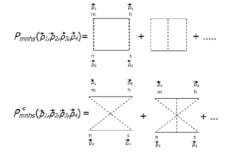
Figure 1: Ladder and maximally crossed diagrams.Dashed line is the correlation function of roughness $W(\vec{\rho}_{1}-\vec{\rho}_{2})$ and the solid line is the averaged over the randomness two-dimensional Green’s function of surface polariton.

It follows from Fig.(1) and the symmetry that $P_{mnhs}(\vec{\rho}_{1},\vec{\rho}_{2},\vec{\rho}_{3},\vec{\rho}_{4})$ can be represented in the form

$$P_{mnhs}(\vec{\rho}_{1},\vec{\rho}_{2},\vec{\rho}_{3},\vec{\rho}_{4})=W(|\vec{\rho}_{1}-\vec{\rho}_{2}|)W(|\vec{\rho}_{3}-\vec{\rho}_{4}|)$$

$$P_{mnhs}\left(\vec{\rho},\vec{\rho}_{1}-\vec{\rho}_{2},\vec{\rho}_{3}-\vec{\rho}_{4}\right)$$ (22)

where $\vec{\rho}=\frac{1}{2}(\vec{\rho}_{3}+\vec{\rho}_{4}-\vec{\rho}_{1}-\vec{\rho}_{2})$. In further we will investigate only the component $P_{zzzz}$ which consists of the diffusion pole and gives the main contribution to the radiation intensity. Using Fig.(1) and Eq.(22) and going to the new variables, see [7], we obtain the following Bethe-Salpeter integral equation

$$\int\frac{d\vec{p}}{(2\pi)^{2}}\left[1-\int\frac{d\vec{q}}{(2\pi)^{2}}f(\vec{q},\vec{K})W(|\vec{p}-\vec{q}|)\right]$$

$$P(\vec{K},\vec{p},\vec{q}^{\,\prime})=f(\vec{q}^{\,\prime},\vec{K})$$ (23)

where $G\equiv G_{zz}$,$P\equiv P_{zzzz}$ and $f(\vec{q},\vec{K})=G(\vec{q}+\frac{\vec{K}}{2})G^{*}(\vec{q}-\frac{\vec{K}}{2})$. Substituting Eqs.(8,22) into Eq.(21) and going to the Fourier transforms, one has

$$I^{D}(\theta,\varphi)=\frac{c}{32\pi^{2}}\frac{(1+n_{\rho}^{2})(1+n_{z}^{2})(1-n_{x}^{2})}{n_{\rho}}\int d\vec{\rho}d\vec{\rho}^{\,\prime}$$

$$\frac{d\vec{p}_{1}d\vec{p}_{2}d\vec{p}_{3}}{(2\pi)^{6}}W(|\vec{\rho}-\vec{\rho}^{\,\prime}|)E_{0z}(0,\vec{\rho})E_{0z}^{*}(0,\vec{\rho}^{\,\prime})P(0,\vec{p}_{1},\vec{p}_{2})$$

$$|G(p_{3})|^{2}e^{i\vec{p}_{3}(\vec{\rho}-\vec{\rho}^{\,\prime})}W(|\vec{p}_{2}+\vec{p}_{3}|)W(|k\vec{n}_{\rho}+\vec{p}_{1}|)$$ (24)

The diffusive propagator $P(\vec{K},\vec{p},\vec{q})$ satisfies the integral equation Eq.(23). In the limit $K\to 0$ one can search its solution in the form [7]

$$P(\vec{K}\to 0,\vec{p},\vec{q})=A(K)\frac{ImG(\vec{p})ImG(\vec{q})}{Im\Sigma(\vec{q})}$$ (25)

where unknown function $A(K)$ should be found from Eq.(23). Substituting Eq.(25) into Eq.(23) and expanding $f(\vec{q},\vec{K})$ up to $K^{2}$ one finds $A(K)$ in the form $A(K)=32/3K^{2}l^{2}$. When obtaining $A(K)$ we calculate integrals in the pole approximation that give main contribution in the weak scattering limit ${\rm Im}\Sigma\to 0$. Substituting Eq.(25) into Eq.(24) and consequently integrating with help of the Word identity Eq.(19) we finally obain for the diffusive contribution

$$I^{D}(\omega,\vec{n})=\frac{4e^{2}}{3\pi^{2}c\beta^{2}}\frac{(1+n_{\rho}^{2})(1+n_{z}^{2})(1-n_{x}^{2})}{n_{\rho}}\frac{L^{2}L_{x}}{l^{2}}$$

$$\frac{{\rm Im}\Sigma(kn_{\rho})}{{\rm Im}\Sigma(k)}F_{1}(\lambda,\sigma,d)$$ (26)

where $L$ is the characteristic size of the system, $L_{x}$ is the system size in the $x$ direction and

$$F_{1}=\left(\frac{dk_{0}}{\gamma}\right)^{2}\int dxdydy^{\prime}\cos(k_{0}x)W(x^{2}+(y-y^{\prime})^{2})$$

$$J_{0}(k\sqrt{x^{2}+(y-y^{\prime})^{2})})\frac{K_{1}(\frac{k_{0}\sqrt{y^{2}+d^{2}}}{\gamma})K_{1}(\frac{k_{0}\sqrt{y^{\prime 2}+d^{2}}}{\gamma})}{\sqrt{(y^{2}+d^{2})(y^{\prime 2}+d^{2})}}$$ (27)

Divergence of diffusive intensity Eq.(24) is caused by the infinite system size , see also [7]. If one takes into account the finite sizes the minimal momentum in the system become equal to $K_{min}\sim 1/L$. We take into account this aspect when obtaining Eq.(26) from Eqs.(24,25).

Comparing single scattering Eq.(4) and diffusive Eq.(26) contributions, one has $I^{D}/I^{0}\sim L^{2}/l^{2}\gg 1$. Hence diffusion of surface polaritons is the main mechanism of radiation.

Note that $F_{1}$ in Eqs.(26,27)does not depend on angle. It is just a number. First we analyze diffusive radiation intensity Eq.(26) in the short wavelength region $k\sigma\gg 1$. Consider the ratio ${\rm Im}\Sigma(kn_{\rho})/{\rm Im}\Sigma(k)\approx\frac{1}{\sqrt{n_{\rho}}}exp\left[-\frac{k^{2}\sigma^{2}}{4}(1-n_{\rho}^{2})\right]$. Because of the exponential function essential intensity is emitted on directions $n_{\rho}\approx 1$, that is parallel to the metal surface. For long wavelengths $k\sigma\ll 1$, on the contrary, maximum is achieved in the direction perpendicular to the surface . Now consider long wavelength region $k\sigma\ll 1$. In this case one can substitute $W_{0}(x^{2}+(y-y^{\prime})^{2})\to\pi\sigma^{2}\delta(x)\delta(y-y^{\prime})$ in Eq.(27). After this simplification, calculating the integrals in Eq.(27), one finds from Eq.(26)

$$I^{D}(\omega,\vec{n})=\frac{2e^{2}}{3c\beta^{2}}\frac{g(1+n_{\rho}^{2})(1+n_{z}^{2})(1-n_{x}^{2})}{n_{\rho}}\frac{L^{2}}{l^{2}}\frac{L_{x}}{d}$$ (28)

Note that we have missed the dimensionless constant $g$ in Eq.(34) of [5] when considering ”white noise” case. Besides that these two expressions differ from each other by a numerical factor. Both these expressions are correct with accuracy up to a numerical factor because the diffusive propagator $P(K\to 0,p,q)$ can be found only with such accuracy.

7 Maximally crossed diagrams contribution

Maximally crossed diagrams, (see Fig.1) contribution to the radiation intensity reads

$$I^{C}(\vec{R})=\int d\vec{\rho}d\vec{\rho}^{\,\prime}d\vec{\rho}_{1}d\vec{\rho}_{2}d\vec{\rho}_{3}d\vec{\rho}_{4}G_{im}^{0}(\vec{R},\vec{\rho}_{1},0)$$ (29)

$$G_{ni}^{*0}(\vec{\rho}_{2},0,\vec{R})P_{mnhs}^{C}(\vec{\rho}_{1},\vec{\rho}_{2},\vec{\rho}_{3},\vec{\rho}_{4})G_{hz}(\vec{\rho}_{3},\vec{\rho})$$

$$G_{zs}^{*}(\vec{\rho}^{\,\prime},\vec{\rho}_{4})W(|(\vec{\rho}-\vec{\rho}^{\,\prime})|)E_{0z}(\vec{\rho},0)E^{*}_{0z}(\vec{\rho}^{\,\prime},0)$$

Due to the time reversal symmetry propagator $P^{C}_{mnhs}$ is related to the diffusive propagator as $P^{C}_{mnhs}(\vec{\rho}_{1},\vec{\rho}_{2},\vec{\rho}_{3},\vec{\rho}_{4})\equiv P_{mshn}(\vec{\rho}_{1},\vec{\rho}_{4},\vec{\rho}_{3},\vec{\rho}_{2})$, see for example,[12]. Calculating analogously to the diffusive contribution case, one has

$$I^{C}(\theta,\omega)=\frac{c}{3\pi^{2}}\frac{(1+n_{\rho}^{2})(1+n_{z}^{2})(1-n_{x}^{2})}{n_{\rho}}\int d\vec{\rho}d\vec{\rho}^{\,\prime}$$ (30)

$$\frac{d\vec{p}_{1}d\vec{p}_{2}d\vec{p}_{3}}{(2\pi)^{6}}W(|\vec{\rho}-\vec{\rho}^{\,\prime}|)E_{0z}(0,\vec{\rho})E_{0z}^{*}(0,\vec{\rho}^{\,\prime})$$

$$\int\frac{d\vec{K}}{(2\pi)^{2}}\frac{{\rm Im}\Sigma(k)}{K^{2}\left[(k^{2}-(\vec{K}-k\vec{n}_{\rho})^{2})^{2}+{\rm Im}\Sigma^{2}(k)\right]}$$

It follows from Eq.(7) that integral over $K$ logarithmically diverges at small $K$. This divergence is manifestation of localisation effects in radiation. It is analogous to the same effects in disordered electronic systems, see for example,[12]. In the weak scattering regime ${\rm Im}\Sigma\to 0$, maximal value of $I^{C}$ is achieved at directions parallel to the surface for which $n_{\rho}$ is close to unity. Cutting integral on $K$ on the bottom limit at $1/L$ and on the upper limit at $1/l$, we finally find from Eq.(7)

$$I^{C}(\theta,\omega)=\frac{2ge^{2}}{3\pi\beta^{2}c}\frac{(1+n_{\rho}^{2})(1+n_{z}^{2})(1-n_{x}^{2})}{n_{\rho}d}\frac{1}{kl}\ln\frac{L}{l}$$ (31)

It follows from Eq.(7) that the peak of angular distribution of $I^{C}$ around the direction $n_{\rho}=1$ has width of order $\sqrt{\lambda/l}$. Remind that the analogous light backscattering peak from a disordered medium in three dimensions has a peak with width $\lambda/l$,see for example, [13]. Remind that our consideration is correct in the weak scattering regime $kl\gg 1$. Therefore maximally crossed diagrams contribution to the radiation intensity is small. However in the light localisation regime $kl\sim 1$ [3] it becomes important because leads to strong frequency dependence of radiation intensity (see below). One can notice the different dependences of single scattering Eq.(4) and diffusive contributions Eqs.(26,7) to radiation intensity on system sizes. The reason of this difference is that in the first case radiation is formed as incoherent sum of intensities from independent scatterers and therefore is proportional to system size or the number of scatterers. In the diffusive radiation case interference terms play important role. They lead to a stronger dependence of the intensity on the system sizes. Therefore diffusive contribution to the radiation intensity can be considered as a type of coherent radiation [15].

8 Spectrum of Radiation

We have assumed that the absorption of electromagnetic field is absent. In this consideration weak $l\ll l_{in}$,where $l_{in}=\varepsilon_{1}^{2}/k\varepsilon_{2}$ is the inelastic mean free path of surface polariton, absorption can be taken into account as follows [14]. When $L>(ll_{in})^{1/2}$, $L$ in Eqs.(26,7) should be substituted by $(ll_{in})^{1/2}$. As was mentioned above in the short wavelength region $k\sigma\gg 1$ the radiation is directed parallel to the surface and its intensity is suppressed compared to the long wavelength $k\sigma\ll 1$ region because the largeness of polariton elastic mean free path. Hence the long wavelength region is more interesting . We will investigate frequency dependence of the radiation intensity in this region. Making the above mentioned substitution and selecting parts depending on the frequency, for the spectral radiation intensity, from Eqs.(15,28,31), one has

$$I_{0}(\omega)\sim g(\omega),\quad I^{D}(\omega)\sim g(\omega)\frac{l_{in}(\omega)}{l(\omega)},$$ (32)

$$I^{C}(\omega)\sim g(\omega)\frac{c}{\omega l(\omega)}\ln\frac{l_{in}(\omega)}{l(\omega)}$$

In order to reveal the frequency dependence of the radiation intensity one has to know the frequency dependences of $g,l$ and $l_{in}$. They depend on dielectric constant $\varepsilon(\omega)$ of isotropic medium which for a single metal is described by Drude formulae $\varepsilon(\omega)=\varepsilon_{1}(\omega)+i\varepsilon_{2}(\omega)=1-\omega_{p}^{2}/\omega(\omega+i\tau^{-1})$, where $\omega_{p}$ and $\tau$ are the plasma frequency and the relaxation time of conduction electrons,respectively. In the optical region we always have $\omega\tau\gg 1$. Therefore, for the real and imaginary parts of dielectric constant one has $\varepsilon_{1}(\omega)\approx 1-\omega_{p}^{2}/\omega^{2}$ and $\varepsilon_{2}\approx\omega_{p}^{2}/\omega^{3}\tau$. Substituting these dependencies into expressions for $g,l$ and $l_{in}$, we find $g\sim constant,\quad l\sim\omega^{-3},\quad l_{in}\sim\omega^{-2}$. Correspondingly, using Eq.(8), one has

$$I_{0}\sim constant,\quad I^{D}(\omega)\sim\omega,\quad I^{C}(\omega)\sim\omega^{2}\ln\omega$$ (33)

It follows from Eq.(33) that the single scattering contribution to radiation intensity does not lead to any frequency dependence $I^{0}(\omega)\sim constant$. In contrary multiple scattering contributions lead to strong dependence of radiation intensity on frequency. Note that strong frequency dependences were observed in early experiments [16] on radiation from rough metallic surfaces. Other radiation mechanisms such as, synchrotron, transition, bremsstrahlung in the optical region do not lead to essential frequency dependence. Only Cherenkov radiation could lead to such dependence. However for the particle moving over a metallic surface in the vacuum it does not exist. This means that the diffusive mechanism can be separated from the other radiation mechanisms. It can be used for monitoring the beam position in the accelerators . Increasing of intensity of the blue part of spectrum would mean that beam have approached to the walls of accelerator. Radiation of non-relativistic electrons from rough surfaces can be used for diagnostic of surface.

9 Summary

We have considered the radiation emission when a charged particle travels above a correlated rough metal surface. It was shown that in the optical region the diffusive mechanism caused by multiple scattering of polaritons on the roughness is the main one. Diffusive radiation is a type of coherent radiation because interference effects play important role in its formation. Both long wavelength $\lambda\gg\sigma$ and short wavelength $\lambda\ll\sigma$ regions were investigated. In the long wavelength region radiation is mainly emitted on the perpendicular to particle velocity direction. In opposite in the short wavelength region maximum of radiation is achieved on the parallel to surface directions. A strong frequency dependence of radiation intensity is found. Its possible application for monitoring of a beam position in accelerators was discussed.

References

• [1] \NameO’Donriel K.A., and Mendez E.R. \REVIEWJ.Opt.Soc.Am. A 4 19871194.
• [2] \NameLi Voti R., Leahu G.L. and et al \REVIEWJ.Opt.Soc.Am. B 26 20091585.
• [3] \NameArya K., Su Z.B. and Birman L. \REVIEWPhys.Rev.Lett. 54 19851559.
• [4] \Name Smith S.J.and Purcell E.M.\REVIEW Phys.Rev. 92 1953 1069.
• [5] \NameGevorkian Zh.S.\REVIEWPhys.Rev.ST Accel.Beams 13 2010 070705.
• [6] \NameMaradudin A.A.and Mills D.L.\REVIEWPhys.Rev.B 11 1975 1392.
• [7] \NameGevorkian Zh.S.\REVIEWPhys.Rev.E 57 1998 2338.
• [8] \NameGevorkian Zh.S.and Nieuwenhuizen Th.M.\REVIEWPhys.Rev.E 61 2000 4656.
• [9] \NameGevorkian Zh.S. and et al\REVIEWPhys.Rev.Lett 97 2006 044801.
• [10] \NameMcGurn A.R., Maradudin A.A. and Celli V. \REVIEWPhys.Rev.B31 19854866.
• [11] \Name Abrikosov A.A.,Gorkov L.P.and Dzyaloshinski I.E. \BookMethods of Quantum Field Theory in Statistical Physics \PublEnglewood Cliffs, New York \Year1963.
• [12] \NameLee P.A. and Ramakrishnan T.V.\REVIEWRev.Mod.Phys.571985287.
• [13] \Namevan Rossum M.C.W. and Nieuwenhuizen Th.M. \REVIEWRev.Mod.Phys.71 1999313.
• [14] \NameAnderson P.W.\REVIEWPhil.Mag521985505.
• [15] \NameTer-Mikaelian M.L. \BookHigh Energy Electromagnetic Processes in Condensed Media \PublWiley and Sons, New York \Year1972.
• [16] \NameHarutunian F.R., Mkhitarian A.Kh.,Hovhanissian R.A., Rostomian B.O. and Sarinyan M.G.\REVIEWSov.Phys.JETP501979895 and references therein.