The mortality of the Italian population: Smoothing techniques on the Lee–Carter model

Abstract

Several approaches have been developed for forecasting mortality using the stochastic model. In particular, the Lee–Carter model has become widely used and there have been various extensions and modifications proposed to attain a broader interpretation and to capture the main features of the dynamics of the mortality intensity. Hyndman–Ullah show a particular version of the Lee–Carter methodology, the so-called Functional Demographic Model, which is one of the most accurate approaches as regards some mortality data, particularly for longer forecast horizons where the benefit of a damped trend forecast is greater. The paper objective is properly to single out the most suitable model between the basic Lee–Carter and the Functional Demographic Model to the Italian mortality data. A comparative assessment is made and the empirical results are presented using a range of graphical analyses.

, and [*]t2Corresponding author.

1 Introduction

In the 20th century, the human mortality has declined globally. Such trends in mortality reduction present risk for insurers which have planned on the basis of historical mortality tables that do not take these trends into account. In this regard, from the life insurance business risk profile point of view, different risk sources have to be evaluated. In particular, life insurance companies and private pension managers deal with the demographic risk, which can be split in two components: the insurance risk and the longevity risk. The insurance risk arises from accidental deviations of the number of the deaths from its expected values, and it is a pooling risk, that is, it can be mitigated by increasing the number of policies.

The longevity risk derives from improvements in the mortality trend, which determine systematic deviations of the number of the deaths from its expected values. These changes clearly affect pricing and reserve allocation for life annuities and represent one of the major threats to a social security system that has been planned on the basis of a more modest life expectancy. The risk is of using mortality tables that do not take these trends into account, thus underestimating the survival probability and determining inappropriate premiums. To face this risk, it is necessary to build projected tables including this trend. Thus, reasonable mortality forecasting techniques have to be used to consistently predict the trends [Brouhns, Denuit and Vermunt (2002)]. In that respect, over the years a number of approaches have been proposed for forecasting mortality using the stochastic model, however, the Lee–Carter model [Lee and Carter (1992)] unquestionably represents a milestone in the literature.

This methodology has become widely used and there have been various extensions and modifications proposed to attain a broader interpretation and to capture the main features of the dynamics of the mortality intensity [e.g., Booth, Maindonald and Smith (2002); Haberman and Renshaw (2003, 2008); Hyndman and Ullah (2007); Renshaw and Haberman (2003a, 2003b)].

The main statistical tool of LC is least-squares estimation via singular value decomposition of the matrix of the log age-specific observed death rates. In fact, the mortality data (death counts and exposures-to-risk) have to fill a rectangular matrix. Henceforth, we will denote with $m_{x,t}$ the observed death rates at age $x$ during calendar year $t$, obtained by the ratio between the number of deaths, $D_{x,t}$, recorded at age $x$ during year $t$, from an exposure-to-risk $E_{x,t}$, that is, the number of person years from which $D_{x,t}$ occurred. As regards the Italian population data set on the basis of the death rates, classified by gender and individual year from $0$ to $100$, plots of fitted values for such models suggest that smoothing is appropriate (see Figures 1 and 2). If we look at Figures 1 and 2, we can notice the random variations in the data, especially for ages between 0 and 10, where the reductions in the death rates are stronger. Moreover, we can notice also for older ages the irregularities are pronounced. These irregularities in fact propagate to the life insurance premiums as well as reserves that have to be held by insurance companies to make them able to pay the future contractual benefit. Consequently, the model fitting on a population has to smooth the random variations in the data, because otherwise the resulting death rates become less reliable.

Figure 1: Italian male death rates, 1950–1965–1985–2000–2005.

The aim of the paper is properly to single out the most suitable model between the basic Lee–Carter (from herein LC) and a variant of this model, the so-called Functional Demographic Model (from herein FDM) by Hyndman–Ullah [Hyndman and Ullah (2007)], to the Italian population demographic trend. In particular, considering the random variations in the data, we can get an extremely accurate fit by using appropriate smoothing techniques. The paper is organized as follows: in Section 2 we describe the LC model and the FDM model; Section 3 shows the traditional P-splines approach for smoothing; in Section 4 a comparative assessment among the basic LC and FDM is performed to the Italian population, by gender separately considered. Concluding remarks are provided in Section 5.

Figure 2: Italian female death rates, 1950–1965–1985–2000–2005.

2 The Lee–Carter model and the Functional Demographic Model

The LC methodology is a milestone in the mortality projections actuarial literature. The model describes the logarithm of the observed mortality rate for age $x$ and year $t$, $m_{x,t}$, as the sum of an age-specific component $\alpha_{x}$, that is independent of time and another component that is the product of a time-varying parameter $\kappa_{t}$, reflecting the general level of mortality and an age-specific component $\beta_{x}$, that represents how mortality at each age varies when the general level of mortality changes:

$$\ln{m_{x,t}}=\alpha_{x}+\beta_{x}\kappa_{t}+\varepsilon_{x,t}.$$ (1)

The $\varepsilon_{x,t}$ component denotes the error term, which is assumed to be homoschedastic and normally distributed. In other words, $\alpha_{x}$ describes the general age shape of the age specific death rates $m_{x,t}$, while $\kappa_{t}$ is an index that describes the variation in the level of mortality to $t$. The $\beta_{x}$ coefficients describe the tendency of mortality at age $x$ to change when the general level of mortality $\kappa_{t}$ changes.

The LC model cannot be fitted by ordinary regression methods, because there are no given regressors on the right-hand side of the equation; thus, in order to find a least squares solution to the equation (1), we use the Singular Value Decomposition (SVD) method, as suggested in Lee and Carter (1992), assuming that the errors are homoschedastic. The parameter uniqueness is specified by a different set of conditions from (1), namely, the sum of the $\beta_{x}$ coefficients is equal to one and the sum of the $\kappa_{t}$ parameters is equal to zero. To forecast mortality by using the LC model, we proceed by following two steps. In the first step, we estimate the parameters $\alpha_{x}$, $\beta_{x}$ and $\kappa_{t}$ using historical mortality data. In the second step, the estimated time-dependent parameter $\kappa_{t}$ is modeled as a stochastic process by an autoregressive integrated moving average (ARIMA p, d, q) model, determined by the standard Box and Jenkins methodology (identification–estimation–diagnosis) [Box and Jenkins (1976); Hamilton (1994)]. Finally, we extrapolate $\kappa_{t}$ through the fitted ARIMA model to obtain a forecast of future death rates and generate associated life table values.

The LC model has become widely used and there have been various extensions and modifications proposed to attain a broader interpretation and to capture the main features of the dynamics of the mortality intensity. Hyndman and Ullah (2007) show a particular version of the LC methodology, the so-called Functional Demographic Model; they propose a methodology to forecast age-specific mortality rates, based on the combination of functional data analysis, nonparametric smoothing and robust statistics. In particular, the approach under consideration allows for smooth functions of age, is robust to outliers and provides a modeling framework easy to fit to constraints and other information.

The modeling framework they propose is a generalization of the LC method. Let $y_{t}(x)$ denote the log of the observed mortality rate for age $x$ and year $t$, $f_{t}(x)$ the underlying smooth function, $\{x_{i},y_{t}(x_{i})\},t=1,\dots,n,i=1,\dots,p$, the functional time series, where

$$y_{t}(x_{i})=f_{t}(x_{i})+\sigma_{t}(x_{i})\varepsilon_{t,i},$$ (2)

with $\varepsilon_{t,i}$ an i.i.d. standard normal random variable and $\sigma_{t}(x_{i})$ allowing for the amount of noise to vary with $x$. The steps for forecasting $y_{t}(x)$ are summarized as follows:

1. The data set is smoothed for each $t$ by applying penalized regression splines. Using a nonparametric smoothing with constraint, we estimate for each $t$ the functions $f_{t}(x)$ for $x\in[x_{1},x_{p}]$ from $\{x_{i},y_{t}(x_{i})\}$ for $i=1,\dots,p$. We assume that $f_{t}(x)$ is monotonically increasing for $x\geq c$ for some $c$ , that is reasonable for mortality data. This constraint allows to reduce the noise in the estimated curves at older ages.

2. The fitted curves are decomposed by using a basis function expansion:

   $$f_{t}(x)=\mu(x)+\sum_{\kappa=1}^{K}{\beta_{t,k}\phi_{k}(x)}+e_{t}(x),$$ (3)

   where $\mu(x)$is a measure of location of $f_{t}(x)$, $\phi_{k}(x)$ is a set of orthonormal basis functions, $\{\beta_{t,k}\}$ are the coefficients and $e_{t}(x)\sim N(0,v(x))$.

3. To each coefficients $\{\beta_{t,k}\},k=1,\ldots,K$, univariate time series models are fitted.

4. On the basis of the fitted time series models the coefficients $\{\beta_{t,k}\},k=1,\dots,K$, are forecasted for $t=n+1,\ldots,n+h$.

5. The coefficients obtained in the previous step are implemented to get the $f_{t}(x)$ as in equation (2). From (2) the $y_{t}(x)$ are projected. In other words, the $y_{t}(x_{i})$ can be expressed as the following formula obtained by combining (2) and (3):

   $$y_{t}(x_{i})=\mu(x_{i})+\sum_{\kappa=1}^{K}{\beta_{t,k}\phi_{k}(x_{i})}+e_{t}(x_{i})+\sigma_{t}(x_{i})\varepsilon_{t,i}.$$ (4)

   In particular, the $h$-steps ahead forecasts of $y_{n+h}(x)$ are given by the formula (5):

   $$\hat{y}_{n+h}(x)=E[y_{n+h}(x)|I,\Phi]=\hat{\mu}(x)+\sum_{\kappa=1}^{K}{\tilde{\beta}_{n,k,h}\hat{\phi}_{k}(x)},$$ (5)

   where $I=\{y_{t}(x_{i});t=1,\dots,n;i=1,\dots,p$, is the observed data, $\Phi$ the set of basis functions, $\tilde{\beta}_{n,k,h}$ corresponds to the $h$-step ahead forecast of $\beta_{n+h,k}$ having been estimated time series $\hat{\beta}_{1,k,},\dots,\hat{\beta}_{n,k,}$.

6. Finally, in order to determine confidence intervals for mortality projections, the variance of error terms in (2) and (3) is calculated. In particular, the forecast variance is written from (4):

   $$\zeta_{n,h}(x)=\operatorname{Var}[y_{n+h}(x)|I,\Phi]=\hat{\sigma}_{\mu}^{2}(x)+\sum_{\kappa=1}^{K}{u_{n+h,k}}\hat{\phi}_{k}^{2}(x)+v(x)+\sigma_{t}^{2}(x),$$ (6)

   where $\hat{\sigma}_{\mu}^{2}(x)$ the variance of the smooth estimate $\hat{\mu}(x)$ depends on the smoothing technique, $u_{n+h,k}=\operatorname{Var}(\beta_{n+h,k}|\beta_{1,k},\dots,\beta_{n,k})$ are obtained by the time series model, being $\sigma_{t}^{2}(x)$ the variance of the $y_{t}(x)$ and the $v(x)$ is the model error variance estimated by averaging $\hat{e}_{t}^{2}(x)$ for each $x$. The prediction interval for $y_{t}(x)$ is represented by the following:

   $$\hat{y}_{n,h}(x)\pm z_{\alpha}\sqrt{\zeta_{n,h}(x)}$$

   assuming normally distributed the sources of error, where $z_{\alpha}$ is the $1-\frac{\alpha}{2}$ standard normal quantile.

   In order to measure the uncertainty in the mortality projections, prediction intervals can be derived applying bootstrap techniques [Efron and Tibshirani (1993)]. They are particularly useful where theoretical calculation with the fitted model is too complex, as in the case where the computation of interval forecast is not straightforward [Koissi, Shapiro and Hognas (2006)].

3 P-splines approach for smoothing

Mortality data are often characterized by the presence of some outlier data. In particular, in the case of older ages, the high variability can be due to the small number of survivors in the population. This represents a common problem when estimating mortality rates for groups aged 90 and more. Techniques of smoothing have been implemented to avoid this shortage of data, because the heavy variance at older ages influences the fitting of mortality models [Delwarde, Denuit and Eilers (2007)].

As suggested by Eilers and Marx (1996), the Penalized splines or P-splines is now well-established as a method of smoothing in Generalized Linear Models. The main characteristics of the methodology under consideration are the following:

1. using B-splines as the basis for the regression;

2. modifying the log-likelihood by a difference penalty on the regression coefficients.

In Currie, Durban and Eilers (2004a, 2004b) the mortality intensity is decomposed as

$$\ln\mu_{x}(t)=\sum_{i,j}{\Theta_{i,j}B_{i,j}(x,t)}$$

for some given 2-dimensional B-splines $B_{i,j}$ in age $x$ and calendar time $t$, with regularly-spaced knots and $\Theta_{i,j}$’s, the parameters to be estimated on the basis of the data set. In order to limit the influence of the knots on the fitted value, Eilers and Marx (1996) suggest to introduce a penality based on finite differences of the coefficients of the adjacent B-spline; this tecnique is called P-spline. For both age and calendar year dimensions, the penalties have to be calculated as sums of $(\Theta_{i,j}-2\Theta_{i-1,j}+\Theta_{i-2,j})^{2}$. For each of these penalties a weight coefficient has to be selected on the basis of the historical data set. Some authors explain that the P-splines are not so transparent to the actuaries, especially because the choice of penalty corresponds to a view of the future pattern of mortality. Currie (2008) shows the limits of using a penalized spline to smooth the mortality data: since the penalty depends on the parameterization, the smoothed value is not invariant with respect to its choice. The solution proposed by Currie is to consider a direct smoothing and replace the penalized differences in the adjacent coefficient with the penalized differences in the adjacent fitted values. Hyndman and Ullah (2007) prefer smoothing the data first, rather than smoothing the fitted values, as it allows to place monotonic constraint on the smoothing more easily.

4 Empirical analysis

We have run the application by considering the Annual Italian male and female mortality rates from $1950$ to $2006$ for single year of age. The data for the Italian population are downloaded from the Human Mortality Database and are described in the Supplementary Material at the end of the paper. We consider death rates for single year of age, for ages from $0$ to $100$. For each gender and for each calendar year, the death rates, given by the ratio between the “Number of deaths” and the “Exposure to risk,” are arranged in a matrix for age and time. By analyzing the changes in mortality as a function of both age $x$ and time $t$, we have seen that mortality has shown a gradual decline over time. To have an idea of this evolution, Figure 1 shows the general drop in the Italian male mortality rates during the period 1950–2005. Improvements in mortality are not uniform across the ages and the years: first of all, reductions in mortality rate are stronger for ages between $0$ and $10$. As it is clear, there is an increasing variance for higher age, especially around $X=100$.

Figure 3: The parameter estimates of basic Lee–Carter model on Italian male mortality data.

The first step of the application consists in fitting the basic LC model and the FDM version to the data under consideration; Figures 3–6 show the estimated parameters.

Figure 4: Basis Functions of FDM and associated coefficients for Italian male population.

Figure 5: The parameter estimates of basic Lee–Carter model on Italian female mortality data.

Figure 6: Basis Functions of FDM and associated coefficients for Italian female population.

The percentage of variation explained by the LC for the male population is 91.6%, while the female is 95.7%. This difference is due to the features of the two data sets: as it is clear from Figures 1 and 2, male death rates show a greater dispersion at older ages than female ones; consequently, the LC model fitted the female data better than the male data. Shifting from the LC to the FDM, the percentage explained by the model increases for both male and female. In particular, if we consider the FDM model, the basis functions explain respectively 91.8%, 3.9%, 1.6%, 0.4% of the variation for male data and 96.0%, 1.6%, 0.4%, 0.3% of the variation for female data. As explained in Hyndman and Ullah (2007), the basis functions model different movements in mortality rates across the ages. In particular, the Basis function 1 mainly models mortality changes for children. Let us have a look at the Figures 3–6, to highlight some differences between female and male death rates. The function fitted on female data has a stronger slope between age $0$ and $10$ than the function fitted on male data, so the reduction in mortality at younger ages is larger for female than for male. Moreover, the fitted coefficient $1$ gives us information about the improvements in mortality at younger age. If we look at the graphs, the mortality rates for children have dropped over the whole period and this phenomenon is captured by the decreasing trend of the first coefficients for both male and female, even if the improvements are stronger for female. Following in the examination of the movements in mortality rates modeled by the basis functions, the Basis function 2 gives us information about the differences between $30$ and $60$ years old, more stressed for female than for male. The other functions are more complex and model differences between all the cohorts; these differences are less significant for female than for male so that the functions $2$ and $3$ show a lower variability between $40$ and $100$. We have implemented the $t$-tests on the standardized residuals for testing the hypothesis of zero mean. The tests run for both male and female and for FDM and LC in all cases have showed $p$-value equal to $1$. On the contrary, the hypothesis of normality of standardized residuals tested with the Shapiro test is always decidedly rejected; this is a well-known limit of this mortality model [Dowd et al. (2010)]. However, either for male or female, there is an improvement in the goodness of the fitting shifting from the LC to the FDM. A good fit is achieved when the residuals are independent and identically distributed. We have verified these conditions using contour maps (see Figures 7 and 8); moreover, we have calculated the error measures shown in Tables 1 and 2 as in Cairns et al. (2009). By comparing the traditional LC model to the FDM one, the percentage of variation explained by the model is higher in the FDM than in LC; in addition, error measures are lower for both the male and female data set.

We keep running the application, in order to verify if the best fitting of FDM depends on the smoothing on the data involved in the model or is due to other causes.

For this reason, we smooth the data using a monotonic P-spline and then we apply the LC method to the smoothed data; we call this procedure LCS. From a first analysis, we can see that the percentage variation explained by applying the LCS model is 93.4% for male and 97.5% for female. In particular, we can notice that the percentage of variance explained increases when we shift from LC to LCS; this is not due to a greater capacity of the model to describe the data, but to a transformation of the same data into data less variable. Nevertheless, the MSE of the LCS is greater than the MSE of the FDM in both data sets.

However, it is quite possible for a model to provide a good in-sample fit to historical data but still produce poor forecasts, that is, forecasts that differ significantly from subsequently realized outcomes. A good model should provide accurate fits to the historical data as well as produce plausible forecasts. Backtesting procedures consider what results would have been produced if the model had been used in the past. We use this approach to test the original LC model, the LCS and the FDM, setting out a backtesting framework that can be used to evaluate the ex-post forecasting performance of the mortality models. The recent literature follows this approach to evaluate the performance of different mortality models. Lee and Miller (2001) evaluated the performance of the Lee–Carter model by examining the behavior of forecast errors comparing some error measures and producing plots of error distributions, although they did not report any formal test. More recently, CMI (2006) included backtesting evaluations of the P-spline model.

In the light of this contribution, we implement a backtesting procedure, based on the following considerations. First of all, it is necessary to select the metric of interest, namely, the forecasted variable that is the focus of the backtest. Possible metrics include the mortality rate, life expectancy, future survival rates, and the prices of annuities and other life-contingent financial instruments. Different metrics are relevant for different purposes, for example, in evaluating the effectiveness of a hedge of longevity or mortality risk an important metrics could be the insurance reserves. In this paper we focus on the mortality rate itself: our aim is to investigate the feasibility of different mortality models rather than quantify the impact of longevity risk on insurance product.

=270pt ME MSE MPE MAPE Average across ages    Male $0.00786$ $0.01947$ $-0.01290$ $0.03697$    Female $0.00190$ $0.01462$ $-$$0.00038$ $0.01694$ Average across years    Male $0.78248$ $1.88518$ $-1.14400$ $3.48655$    Female $0.18968$ $1.40760$ $-$$0.02626$ $1.59764$

Table 1: Lee–Carter model

=270pt ME MSE MPE MAPE Average across ages    Male $0.00001$ $0.00367$ $-0.01037$ $0.02764$    Female $0.00001$ $0.00403$ $-$$0.00070$ $0.01145$ Average across years    Male $0.00101$ $0.30953$ $-0.85270$ $2.48752$    Female $0.00115$ $0.34586$ $-$$0.05956$ $1.02922$

Table 2: Functional Demographic Model

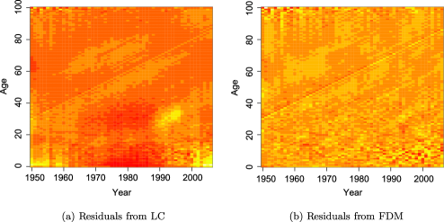
Figure 7: Residuals for male data set.

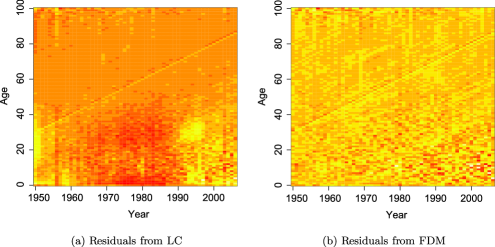
Figure 8: Residuals for female data set.

Another important point is the selection of the historical “lookback” window and the forecast horizon over which forecasts are made. Wang and Liu (2010) highlight that as the fitted period changes, models that better perform change. In the present paper, we focus on long-horizon forecasts, because it is with the accuracy of these forecasts that pension plans and life insurance companies are principally concerned. In particular, we fit the LC, LCS and FDM from $1950$ to $1975$, thereby using a $25$ year in-sample period, then we project the mortality rates with 95% confidence interval from $1976$ to $2005$ according to the fitted models and compare projections with the observed rates. It is necessary to highlight that projections are based only on the evolution of $k_{t}$: errors in $a_{x}$ and $b_{x}$ are not taken into account. In this regard, Lee and Carter (1992) found the standard errors of $a_{x}$ and $b_{x}$ to become less significant over forecast time in comparison to the standard error of $k_{t}$. Moreover, they found that by $10$ years into the forecast of US mortality, $98$ per cent of the standard error of life expectancy at birth was accounted for by uncertainty in $k_{t}$. Figures 9–11 show the forecast error in the LC, LCS and FDM for both male and female. In order to compare the forecast accuracy between LC, LCS and FDM, we calculate the forecasting errors; these are averaged over forecast years to produce mean errors indexed by age. Moreover, we consider mean forecast errors in life expectancy at birth averaging over forecast years.

Figure 9: LC Forecast errors for male and female.

Figure 10: LCS Forecast errors for male and female.

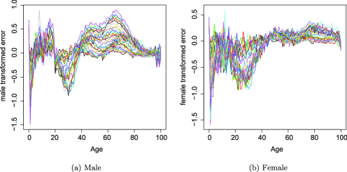
Figure 11: FDM Forecast errors for male and female.

Figure 12 shows the mean forecast error by age. Shifting from LC or LCS to FDM, a large improvement in the male forecasts accuracy in terms of mean forecast error is obtained for ages between $75$ and $98$; improvements also appear for the female data set, where the mean forecast error produced by FDM is smaller than those produced by LC or LCS almost everywhere.

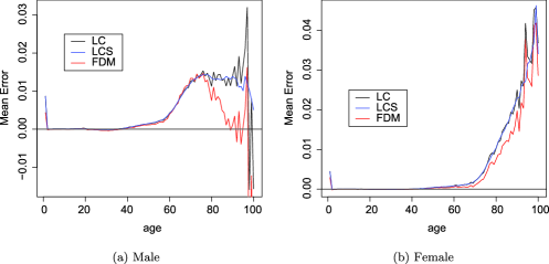
Figure 12: Mean Forecast Error for male and female.

Figure 13 shows the standard deviation of forecast error by age: the variability in the forecasts is smaller in FDM than in LC or LCS for both male and female almost everywhere. Tables 3 and 4 summarize the mean and variance of forecast error in life expectancy. The negative mean error in life expectancy forecast means that the original LC model underestimates the life expectancy and this results in underestimating the capital required for cushioning against longevity risk. However, this underestimation appears smaller for FDM for both male and female data sets; moreover, shifting from LC or LCS to FDM, the variance of forecast errors decreases. Finally, we derive prediction intervals as in Lee and Carter (1992) and Hyndman and Ullah (2005). The confidence interval is calculated at a level of 95%. As shown in Figures 14 and 15, the interval forecasts for the life expectancy at birth from the LC are significantly wider than those from FDM.

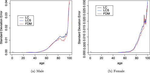
Figure 13: Standard deviation of Forecast Error for male and female.

=255pt LC LCS FDM Mean $-3.210096$ $-3.215095$ $-2.507768$ Variance $-$$1.693628$ $-$$1.691588$ $-$$1.612351$

Table 3: Forecast error in life expectancy at birth for male data set

=255pt LC LCS FDM Mean $-1.632653$00, $-1.637128$ $-1.010379$ Variance $0.6561454$ 0,$0.654672$ ,$0.49403$

Table 4: Forecast error in life expectancy at birth for female data set

5 Concluding remarks

In Life Insurance, primary is the relevance of the demographic uncertainty on the portfolio liability valuations both in its systematic and unsystematic face. The unsystematic component of the demographic risk seems to be a risk source particularly interesting in small portfolios, like the one at issue, for which a weak diversification can be supposed. Unlike the risks deriving from systematic variability, the risk due to the accidental deviations of the number of deaths from the expected values (Mortality risk) is a pooling risk, for which the measure becomes negligible only when the number of contracts in the portfolio tends to infinity. The systematic component originates from the deviations of the number of deaths from the expected values due to the improvement in the survival trend, taking place in the industrialized countries particularly in the last decades. The correct capital constraint, avoiding to reserve more than necessary, derives from the choice of the right mortality table, that is, from the best mortality estimate. This risk source comes true in the survival description choice and it is called Longevity risk. When living benefits are concerned, the calculation of expected present values (needed in pricing and reserving) requires an appropriate mortality projection in order to avoid underestimation of future costs. In order to protect the company from mortality improvements, actuaries have to resort to life tables including a forecast of the future trends of mortality (the so-called projected tables). Different approaches for building these technical bases have been developed by actuaries and demographers.

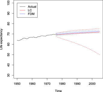
Figure 14: Confidence intervals for male life expectancy.

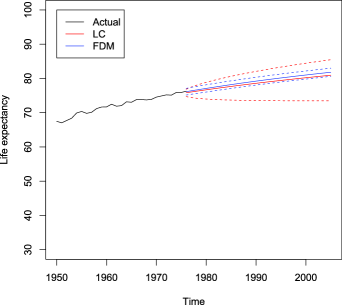
Figure 15: Confidence intervals for female life expectancy.

This paper focuses on a comparative assessment among the original LC model and a variant of the basic methodology, the so-called FDM, for providing accurate mortality forecasting, as regards the Italian survival phenomenon. While it is essential to safeguard against depicting general conclusions on the basis of individual cases, the analysis furnishes a useful insight into the comparative performance of the different approaches under consideration. In order to perform the numerical analysis, we have used the demography R created by Hyndman, Booth Tickle and Maindonald (http://robjhyndman.com/software/demography/).

The empirical results suggest the FDM framework is readily suitable to deal with more complex forecasting problems, including forecasting of the mortality dynamics related to extreme ages. In particular, the FDM methodology utilizes penalized regression to smooth data using a local algorithm which allows for contemporarily the best fitting and a fast computational form. Although the LC is still used as a point of reference [e.g., Renshaw and Haberman (2003b)], it is noted the best performance of the FDM model. According to our analysis applied to male and female Italian data, we have verified that FDM data sets produce a better fitting and more accurate forecasts than LC. We have highlighted that this improvement is not only due to smoothing, introducing a smoothing version of the Lee–Carter (LCS). In fact, we have obtained a better fitting and more accurate forecast also shifting from LCS to FDM and this because FDM explains better movements in the mortality through the basis functions in both data sets.

The study suggests that the FDM forecast accuracy is arguably connected to the model structure, combining functional data analysis, nonparametric smoothing and robust statistics. In particular, the decomposition of the fitted curve via basis functions represents the advantage, since they capture the variability of the mortality trend, by separating out the effects of several orthogonal components. The empirical findings suggest the FDM framework is readily adapted to deal with more complex forecasting problems, including forecasting of the mortality dynamics related to extreme ages.

From the viewpoint of insurance companies, this model feature is more desirable, because of their exposure to the variability of mortality trend at old ages, in particular regards to post retirement annuity-type products. [id=suppA] Supplement A Italy, Exposure to risk [doi]10.1214/10-AOAS394SUPPA [url]http://lib.stat.cmu.edu/aoas/394/supplementA.txt .txt Italian population exposed to risk of death. The data are downloaded from the Human Mortality database and are indexed by calendar year during the period 1950–2005. They are divided by sex and by single year of age for ages from 0 to 100. [id=suppB] Supplement B Italy, Death rates [doi]10.1214/10-AOAS394SUPPB [url]http://lib.stat.cmu.edu/aoas/394/supplementB.txt .txt Italian population death rates. The data are downloaded from the Human Mortality database and are indexed by calendar year during the period 1950–2005. They are divided by sex and by single year of age for ages from 0 to 100. For each gender and for each calendar year, the death rates are given by the ratio between the “Number of deaths” and the “Exposure to risk.”

References

- (1) Booth, H., Maindonald, J. and Smith, L. (2002). Applying Lee–Carter under conditions of variable mortality decline. Population Studies 56 325–336.
- (2) Box, G. E. P and Jenkins, G. M. (1976). Time Series Analysis for Forecasting and Control. Holden-Day, San Francisco. \MR0436499
- (3) Brouhns, N., Denuit, M. and Vermunt, J. K. (2002). A Poisson log-bilinear regression approach to the construction of projected life tables. Insurance Math. Econom. 31 373–393. \MR1945540
- (4) Cairns, A., Blake, D., Dowd, K., Coughlan, G. D., Epstein, D., Ong, A., Balevich I., Brouhns, N., Denuit, M. and Vermunt, J. K. (2009). A quantitative comparison of stochasting mortality models using data from England and Wales and the United States. N. Amer. Actuar. J. 13 1–35.
- (5) CMI (2006). Stochastic projections methodologies: Further progress and P-spline model feature, example results and implications. Working Paper 20, Continuous Mortality Investigation.
- (6) Currie, I. D., Durban, M. and Eilers, P. H. C. (2004a). Smoothing and forecasting mortality rates. Statist. Model. 4 279–298. \MR2086492
- (7) Currie, I. D., Durban, M. and Eilers, P. H. C. (2004b). Generalized linear array models with applications to multidimensional smoothing. J. Roy. Statist. Soc. Ser. B 68 259–280. \MR2188985
- (8) Currie, I. D., (2008). Smoothing overparameterized regression models. In Proceedings of 23rd International Workshop on Statistical Modelling, Utrecht, 194–199.
- (9) Delwarde, A., Denuit, M. and Eilers, P. (2007). Smoothing the Lee–Carter and Poisson log-bilinear models for mortality forecasting. Statist. Model. 7 29–48.
- (10) Dowd, K., Blake, D., Cairns, A. J. G., Eilers, P. H. C. and Marx, B. D. (2010). Facing up to uncertain life expectancy: The longevity fan charts. Demography 47 67–78.
- (11) Efron, B. and Tibshirani, R. J. (1993). An Introduction to the Bootstrap. Chapman and Hall, London. \MR1270903
- (12) Eilers, P. H. C. and Marx, B. D. (1996). Flexible smoothing with B-splines and penalties. Statist. Sci. 11 89–121. \MR1435485
- (13) Haberman, S. and Renshaw, A. E. (2003). On the forecasting of mortality reduction factors. Insurance Math. Econom. 32 379–401.
- (14) Haberman, S. and Renshaw, A. E. (2008). On simulation-based approaches to risk measurement in mortality with specific reference to Poisson Lee–Carter modelling. Insurance Math. Econom. 42 797–816.
- (15) Hamilton, J. D. (1994). Time Series Analysis. Princeton Univ. Press, Princeton, NJ. \MR1278033
- (16) Hyndman, R. J. and Ullah, S. (2007). Robust forecasting of mortality and fertility rates: A functional data approach. Comput. Statist. Data Anal. 51 4942–4956.
- (17) Koissi, M. C., Shapiro, A. F. and Hognas, G. (2006). Evaluating and extending the Lee–Carter model for mortality forecasting: Bootstrap confidence interval. Insurance Math. Econom. 26 1–20. \MR2197300
- (18) Lee, R. D. and Carter, L. R. (1992). Modelling and forecasting US mortality. J. Amer. Statist. Assoc. 87 659–671.
- (19) Lee R. D. and Miller, T. (2001). Evaluating the performance of the Lee–Carter method for forecasting mortality. Demography 38 537–549.
- (20) Renshaw, A. E. and Haberman, S. (2003a). Lee–Carter mortality forecasting: A parallel generalised linear modelling approach for England and Wales mortality projections. Appl. Statist. 52 119–137. \MR1959085
- (21) Renshaw, A. E. and Haberman, S. (2003b). Lee–Carter mortality forecasting with age specific enhancement. Insurance Math. Econom. 33 255–272. \MR2039286
- (22) Wang, C. and Liu, Y. (2010). Comparison of mortality modelling and forecasting—empirical evidence from Taiwan. Lee–Carter mortality forecasting with age specific enhancement. Int. Res. J. Fin. Econ. 37 46–55.