X-ray properties of

the Sun and some compact

objects of our Galaxy

Ph.D. Thesis under the supervision of
Prof. Sandip K. Chakrabarti

Thesis submitted for the degree of
Doctor of Philosophy (Science)
in Physics (Theoretical) of the
Calcutta University

Dipak Debnath

Indian Centre for Space Physics

43-Chalantika, Garia Station Road

Kolkata-700084, India

2010

I want to dedicate this thesis to parents.

ABSTRACT

Sun is the closest and the brightest star from us. Even though its surface temperature is only $\sim 6000$K, it emits X-rays and $\gamma$-rays up to a few Mev. This is primarily because of many non-thermal processes and rapid magnetic reconnections which may produce energetic solar activities. Apart from the thermal electrons which obey Maxwell-Boltzmann distribution, the charged particles, especially electrons are accelerated by shocks and acquire a non-thermal (power-law) distribution. These non-thermal electrons emit energetic synchrotron emissions. With time, the energy is shifted from one wavelength to another. One of our goals is to understand the energy transport processes on the solar surface through detailed observation. It is due to plasma oscillations, or pinching or sausage instabilities in the magnetic field. For the study of temporal and spectral behaviours of the Sun, three detector payloads (two phoswich type payloads (RT-2/S, RT-2/G) and one solid state imaging type payload (RT-2/CZT) with detectors CZT & CMOS) and one control electronic payload (RT-2/E) developed by Indian scientists. As a whole, these four Indian payloads are called RT-2 and have been developed by Tata Institute of Fundamental Research (TIFR), Indian Centre for Space Physics (ICSP) in association with Vikram Sarabhai Space Centre (VSSC). RT-2 onboard Russian CORONAS-PHOTON Mission Satellite was successfully launched on $30^{th}$ January, 2009. These payloads observe the Sun mainly in the X-ray band of 15-150 keV. I have worked on the development of the RT-2 system from its very beginning stage to its final Flight Model stage at ICSP (Kolkata) and at the same time had to visit several national laboratories, namely, VSSC, SAC, PRL, TIFR (Mumbai). My thesis contains the details of the development of RT-2 payloads along with some interesting scientific results what we got so far from these payloads.

RT-2/CZT is the only imaging payload of the RT-2 system with very high spacial and spectral resolutions. For the first time in the history of space-borne instruments, Fresnel Zone Plates (FZPs) were used as an imaging coder in RT-2/CZT. In RT-2/CZT, coded aperture masks (CAMs) were also used as coders for Cadmium Zinc Telluride (CZT) detectors. Before using these shadow cast imaging techniques, we made theoretical simulations (using Monte Carlo method) and experimental set-ups. These results has been discussed in Chapter 2, briefly.

Due to completely different reason, astrophysical black holes (BHs), which are not supposed to emit any radiation, are also sources of very high energy X-rays. It turns out that the matter which falls into the black holes emits the radiation. The process of capturing matter by gravitating objects is called accretion. In steady states, a disk-like structure is formed around black holes. This is called the accretion disk. These disks primarily contain two components: one having a Keplerian angular momentum distribution, emits a multi-colour black body radiation due to its high optical thickness. The other component is sub-Keplerian, which is hot and lesser efficient in emitting radiation. Even though there is no boundary layer of a black hole in the usual sense, the matter between the centrifugal barrier and the horizon behaves as the boundary layer. This is called CENtrifugal pressure supported BOundary Layer or CENBOL. The hot electrons of CENBOL intercept soft photons from the Keplerian disk and the synchrotron radiation from gyrating electrons and re-emit them as hard X-rays or $\gamma$-rays in the form of a power-law component. In my Thesis, I am going to present the results on the stellar mass black holes with its mass ranging from 3 to 20 times the mass of the sun. Out of a dozen of confirmed black hole candidates in our own galaxy, our aim is to study outburst and variable sources such as GRO J1655-40 and GX 339-4, which show flare like events in a much shorter time scale.

In Chapter 1 of my Thesis, we gave an introduction of the subject “Astronomy and Astrophysics”. Also we gave introductions on the X-ray properties, physical processes, theoretical models and missions involved for studying the Sun, the GRBs and the black hole X-ray binaries.

In Chapter 2, we discuss the details of the space instruments (RT-2 for solar science and GRB study & RXTE for black hole study), their data acquisition methods and analysis procedures, whose data we have used during the Ph.D. period.

In Chapter 3, we present the observational results (only solar science) obtained so far using the RT-2 instruments.

Chapter 4 is devoted for the black hole study. In this Chapter, we have discussed the results obtained from our detailed timing and spectral study of 2005 outburst of the black hole candidate GRO J 1655-40.

In Chapter 5, we discuss the results obtained from timing and spectral study of the transient outburst source GX 339-4, during the initial phase of the on-going 2010 outburst.

Finally, in Chapter 6, we make concluding remarks and a brief plan of my future works.

ACKNOWLEDGMENTS

It is great pleasure for me to express my heartiest gratitude to my thesis supervisor Prof. Sandip K. Chakrabarti for his inspiring guidance, constant support and immense patience throughout the years of my Ph.D. period. I am very grateful to him for setting up ambitious goals for me and helping me find out my own way to achieve them.

It is also my pleasure to thank all the academic and non-academic staff of Indian Centre for Space Physics (ICSP) for their enthusiastic support during my studies here. I also thank Prof. J. N. Chakrabarty (Vice President, ICSP).

My sincerest greetings goes to Prof. A. R. Rao of Tata Institute of Fundamental Research (TIFR), Mumbai, PI and Prof. S.K. Chakrabarti (SNBNCBS and ICSP) for giving me opportunity to work as a team member of the RT-2 Developmental team. It is a rare opportunity to develop space instruments which worked well and sent valuable data.

I am thankful to Prof. A. Vacchi of INFN, Trieste, Italy and Director of ICTP for giving me opportunities to work at mlab, the Abdus Salam International Centre for Theoretical Physics (ICTP), Trieste, Italy on Silicon Drift Detector (SDD) during my repeated visits. This also helped me very much for enriching my knowledge for developing large area, high sensitive and high resolution of space borne instrument. I also want to thank Dr. N. Zampa for his kind collaboration at mlab.

I am also thankful to Dr. Anuj Nandi, Dr. Samir Mandal, Mr. Broja Gopal Dutta, Mr. Ritabrata Sarkar and Mr. Partha Sarathi Pal of ICSP for their kind collaboration during my Ph.D. activities at ICSP. My heartiest thanks go to my friends and colleagues at ICSP, with whom I have spend beautiful moments during my Ph.D. period. In this regard, I do not like to mention anyone name or events as they are truly countless. I have shared many ‘unforgettable’ moments and I would like to keep them in my memory forever. But I should mention the name of Dr. Ankan Das whose company enlivened me very often and Mr. Debashis Bhowmick who has shared beautiful moments with me at ICSP and ICTP.

I should thank all my colleagues, past and present, in the astrophysics group of ICSP. Specially I would like to mention the name of Dr. Anuj Nandi whose friendly guidance helped me to carry out my thesis work smoothly. Among the others, I must mention the name of Dr. Samir Mandal, Dr. Sabyasachi Pal and Mr. Tilak Ch. Kotoch of ICSP with whom I had fruitful discussions on various aspects of astronomy and astrophysics.

Finally, I should acknowledge “Council for Scientific and Industrial Research” (CSIR) for giving me full financial support and ICTP, Italy for giving a partial financial support for carry out my thesis work.

I thank my loving parents, Late Nanda Dulal Debnath and Dulali Debnath, for their continuous support from my childhood and making me as a good human. They help me to become an independent person to take all the decisions in my life. But it is a great sorrow to me that I lost my father few months before the submission of this Thesis, who motivated me a lot in doing research. Although he was a good student, did not able to continue his study due to poverty. So, I always tried to reduce his unhappiness with my success. I also thank to my elder brother Hari Har Debnath and my sister-in-law, for their continuous support to my study. Also I want to thank to my niece Hritika Debnath, who gave me a lot of love and pleasure to my life. A special thank goes to my wife Mrs. Moumita Debnath for her constant inspiration. Among the other family members, I want to thank to my grant mother Brojabala Debnath, father-in-law Parimal Debnath, mother-in-law ITI Debnath and brother-in-law Partha Debnath.

Last but not the least I would like to acknowledge ‘myself’, without whose unfailing inner motivation this work could not have been completed.

PUBLICATIONS IN REFEREED JOURNALS

1. Propagating oscillatory shock model for QPOs in GRO J1655-40 during the March 2005 outburst by S. K. Chakrabarti, A. Nandi, D. Debnath, R. Sarkar and B. G. Datta in Indian J. Phys., 79(8), 841-845 (2005) (arXiv: astro-ph/0508024).

2. Evolution of the quasi-periodic oscillation frequency in GRO J1655-40 - - Implications for accretion disk dynamics by S. K. Chakrabarti, D. Debnath, A. Nandi and P. S. Pal in A$\&$A, 489, L41-L44 (2008) (arXiv: astro-ph/0809.0876).

3. Timing and Spectral evolution of GRO J1655-40 during recent 2005 outburst by D. Debnath, S. K. Chakrabarti, A. Nandi and S. Mandal in BASI, 36, 151 (2008) (arXiv: astro-ph/0902.3791).

4. Fresnel Zone Plate Telescopes for X-ray Imaging I: Experiments with a quasi-parallel beam by S. K. Chakrabarti, S. Palit, D. Debnath, A. Nandi and V. Yadav in Exp. Astron., 24, 109 (DOI 10.1007/s10696-009-9144-y) (2009) (arXiv: astro-ph/0910.1987).

5. Fresnel Zone Plate Telescopes for X-ray Imaging II: Results of numerical simulations by S. Palit, S. K. Chakrabarti, D. Debnath, A. Nandi, V. Yadav, V. Girish and A. R. Rao in Exp. Astron., 27, 77 (DOI 10.1007/s10686-009-9176-3) (2009) (arXiv: astro-ph/0910.2353).

6. RT-2 Detection of Quasi-Periodic Pulsations in the 2009 July 5 Solar Hard X-ray Flare by A. R. Rao, J. P. Malkar, M. K. Hingar, V. K. Agrawal, S. K. Chakrabarti, A. Nandi, D. Debnath, T. B. Kotoch, T. R. Chidambaram, P. Vinod, S. Sreekumar, Y. D. Kotov, A. S. Buslov, V. N. Yurov, V. G. Tyshkevich , A. I. Arkhangelskij, R. A. Zyatkov, S. S. Begum, P. K. Manoharan in ApJ, 714, 1142 (2010) (arXiv: astro-ph/1003.3992).

7. Properties of the Propagating Shock wave in the accretion flow around GX 339-4 in 2010 outburst by D. Debnath, S. K. Chakrabarti and A. Nandi in A$\&$A, 520, 98 (DOI 10.1051/0004-6361/201014990) (2010) (arXiv: astro-ph/1009.3351).

8. Instruments of RT-2 Experiment onboard CORONAS-PHOTON and their test and evaluation I: RT-2/S and RT-2/G Payloads by D. Debnath, A. Nandi, A. R. Rao, J. P. Malkar, M. K. Hingar, T. B. Kotoch, S. Sreekumar, V. P. Madhav and S. K. Chakrabarti in Exp. Astron. (in press) (DOI 10.1007/s10686-010-9205-2) (2010) (arXiv: astro-ph/1011.3326).

9. Instruments of RT-2 Experiment onboard CORONAS-PHOTON and their test and evaluation II: RT-2/CZT Payload by T. B. Kotoch, Anuj Nandi, D. Debnath, J. P. Malkar, A. R. Rao, M. K. Hingar, V. P. Madhav, S. Sreekumar and S. K. Chakrabarti, in Exp. Astron. (in press) (DOI 10.1007/s10686-010-9189-y) (2010) (arXiv: astro-ph/1011.3331).

10. Instruments of RT-2 Experiment onboard CORONAS-PHOTON and their test and evaluation III: Coded Aperture Mask and Fresnel Zone Plates in RT-2/CZT Payload by A. Nandi, S. Palit, D. Debnath, S. K. Chakrabarti, T. B. Kotoch, R. Sarkar, V. Yadav, V. Girish, A. R. Rao and D. Bhattacherya in Exp. Astron. (in press) (DOI 10.1007/s10686-010-9184-3) (2010) (arXiv: astro-ph/1011.3338).

11. Instruments of RT-2 Experiment onboard CORONAS-PHOTON and their test and evaluation IV: Background Simulations using GEANT-4 Toolkit by R. Sarkar, S. Mandal, D. Debnath, T. B. Kotoch, A. Nandi, A. R. Rao, S. K. Chakrabarti, in Exp. Astron. (in press) (DOI 10.1007/s10686-010-9208-z) (2010) (arXiv: astro-ph/1011.3340).

12. Instruments of RT-2 Experiment onboard CORONAS-PHOTON and their test and evaluation V: Onboard software, Data Structure, Telemetry and Telecommand by S. Sreekumar, P. Vinod, E. Samuel, J. P. Malkar, A. R. Rao, M. K. Hingar, V. P. Madhav, D. Debnath, T. B. Kotoch, A. Nandi, S. S. Begum and S. K. Chakrabarti, in Exp. Astron. (in press) (DOI 10.1007/s10686-010-9185-2) (2010) (arXiv: astro-ph/1011.3344).

13. Detection of GRB 090618 with RT-2 Experiment Onboard the Coronas - Photon Satellite by A. R. Rao, J. P. Malkar, M. K. Hingar, V. K. Agrawal, S. K. Chakrabarti, A. Nandi, D. Debnath, T. B. Kotoch, R. Sarkar, T. R. Chidambaram, P. Vinod, S. Sreekumar, Y. D. Kotov, A. S. Buslov, V. N. Yurov, V. G. Tyshkevich, A. I. Arkhangelskij, R. A. Zyatkov, S. Naik ApJ (in press) (2010) (arXiv: astro-ph/1012.0461).

14. Onboard performance of the RT-2 detectors by A. R. Rao, J. P. Malkar, M. K. Hingar, V. K. Agrawal, S. K. Chakrabarti, A. Nandi, D. Debnath, T. B. Kotoch, R. Sarkar, T. R. Chidambaram, P. Vinod, S. Sreekumar, Y. D. Kotov, A. S. Buslov, V. N. Yurov, V. G. Tyshkevich, A. I. Arkhangelskij, R. A. Zyatkov (2010, Submitted to Solar System Research).

15. Spectral and Timing evolution of GX 339-4 during its 2010 outburst by D. Debnath, S.K. Chakrabarti and A. Nandi (2010, in preparation).

16. Oscillations of the Compton Cloud During Quasi-Periodic Oscillations in black hole candidates by D. Debnath, S. K. Chakrabarti and P. S. Pal (2010, in preparation).

PUBLICATIONS IN JOURNAL PROCEEDINGS

1. Spectral and QPO Properties of GRO J1655-40 in the 2005 Outburst by S. K. Chakrabarti, A. Nandi, D. Debnath, R. Sarkar and B. G. Datta in VI Microquasar Workshop (Microquasars and Beyond) from September 18-22, 2006 at Società Casino, Como, Italy [POS 103 (2006)].

2. Quasi Periodic Oscillations due to Axisymmetric and non-axisymmetric shock oscillations in black hole accretion by S. K. Chakrabarti, D. Debnath, P. S. Pal, A. Nandi, R. Sarkar, M. M. Samanta, P. J. Witta, H. Ghosh and D. Som in $11^{th}$ Marcel Grossman Meeting on General Relativity from July 23-29, 2006 at Freie Universitaet, Berlin, Germany [World Scientific, 569 (2008)].

3. Solar Science using RT-2 payloads abroad Coronas-photon satellite by D. Debnath, A. Nandi, S. K. Chakrabarti, A. R. Rao and P. K. Manoharan, in Proc. $25^{th}$ meeting of ASI [BASI, 25S, 82 (2008)].

4. Fresnel zone plates: their suitability for X-ray imaging by P. S. Pal, D. Debnath, A. Nandi, V. Yadav, S. K. Chakrabarti, A. R. Rao and V. Girish in Proc. $25^{th}$ meeting of ASI [BASI, 25S, 83 (2008)].

5. Background simulation of the X-ray detectors using Geant4 toolkit by R. Sarkar, S. Mandal, A. Nandi, D. Debnath, S. K. Chakrabarti and A. R. Rao in Proc. $25^{th}$ meeting of ASI [BASI, 25S, 83 (2008)].

6. QPO Evolution in 2005 Outburst of the Galactic Nano Quasar GRO J1655-40 by D. Debnath, A. Nandi, P. S. Pal and S. K. Chakrabarti in proceeding of the Second Kolkata Conference on “Observational Evidence for Black Holes in the Universe” from February 10-15, 2008 at Vedic village and Radisson fFort, Kolkata, India [AIP Conf. Proc. 1053, 171 (2008)].

7. Fresnel Zone Plates for Achromatic Imaging Survey of X-ray sources by S. Palit, S. K. Chakrabarti, D. Debnath, V. Yadav and A. Nandi in proceeding of the Second Kolkata Conference on “Observational Evidence for Black Holes in the Universe” from February 10-15, 2008 at Vedic village and Radisson fFort, Kolkata, India [AIP Conf. Proc. 1053, 391 (2008)].

8. CSPOB - Continuous Spectrophotometry of Black Holes by S. K. Chakrabarti, D. Bhowmick, D. Debnath, R. Sarkar, A. Nandi, V. Yadav and A. R. Rao in proceeding of the Second Kolkata Conference on “Observational Evidence for Black Holes in the Universe” from February 10-15, 2008 at Vedic village and Radisson fFort, Kolkata, India [AIP Conf. Proc. 1053, 409 (2008)].

9. Indian Payloads (RT-2 Experiment) Onboard CORONAS-PHOTON Mission by A. Nandi, A. R. Rao, S. K. Chakrabarti, J. P. Malker, S. Sreekumar, D. Debnath, T. B. Kotoch, Y. Kotov and A. Arkhangelsky, in proceeding of 1st International Conference of Space Technology from August 24-26, 2009 at Electra Palace Hotel, Thessaloniki, Greece (IEEE) (2009) (arXiv: astro-ph/0912.4126).

10. Fresnel Zone Plate Telescopes as high resolution imaging devices by S.K. Chakrabarti, S. Palit, A. Nandi, V. Yadav and D. Debnath, in proceeding of 1st International Conference of Space Technology from August 24-26, 2009 at Electra Palace Hotel, Thessaloniki, Greece (IEEE) (2009) (arXiv: astro-ph/0912.4127).

11. RT-2 Observations of gamma-ray bursts by S.K. Chakrabarti, A.R. Rao, V.K. Agrawal, A. Nandi, D. Debnath, T. B. Kotoch, S. Sreekumar, Y. Kotov and A.S. Buslov, in proceeding of 38th COSPAR Scientific Assembly from 18-25 July, 2010 at Bremen, Germany (2010).

12. RT-2 Observations of solar flares by S.K. Chakrabarti, A.R. Rao, V.K. Agrawal, A. Nandi, D. Debnath, T. B. Kotoch, S. Sreekumar, Y. Kotov, A. Arkhangelsky, A. S. Buslov, E. M. Oreshnikov, V. Yurov, V. Tyshkevich, P. K. Manoharan and S. S. Begum, in proceeding of 38th COSPAR Scientific Assembly from 18-25 July, 2010 at Bremen, Germany (2010).

13. Simultaneous observation of Solar Events by Indian Payload (RT-2) and by ICSP-VLF receiver by A. Nandi, S. K. Chakrabarti, D. Debnath, T. B. Kotoch, A. R. Rao, S. K. Mondal, S. Maji and S. Sasmal in proceeding of Very Low Frequency Radio Waves: Theory $\&$ Observations (VELFRATO-10) from March 13-18, 2010 at S.N. Bose National Centre for Basic Sciences, Kolkata, India [AIP Conf. Proc. 1286, 200 (2010)].

14. Gamma-Ray Bursts from RT-2 payloads and VLF signals by T. B. Kotoch, S. K. Chakrabarti, A. Nandi, D. Debnath in proceeding of Very Low Frequency Radio Waves: Theory $\&$ Observations (VELFRATO-10) from March 13-18, 2010 at S.N. Bose National Centre for Basic Sciences, Kolkata, India [AIP Conf. Proc. 1286, 339 (2010)].

15. The Use of Reconfigurable Virtual Instruments for Low Noise, High Resolution Charge Sensitive Amplification by A. Olufemi, D. Bhowmick, D. Debnath, M. L. Crespo, A. Cicuttin and A. Sen in proceeding of Programme FPGAworld’2010 Stockholm on 2010 September 8 at Electrum Kista, Stockholm, Sweden.

PUBLICATIONS IN GCN CIRCULARS ARCHIVE

1. Detection of GRB 090618 by RT-2 Experiment onboard the CORONAS PHOTON Satellite by A. R. Rao, J. P. Malkar, M. K. Hingar, V. K. Agrawal, S. K. Chakrabarti, A. Nandi, D. Debnath, T. B. Kotoch, T. R. Chidambaram, P. Vinod, S. Sreekumar, Y. D. Kotov, A. S. Buslov, V. N. Yurov, V. G. Tyshkevich, A. I. Arkhangelskij, R. A. Zyatkov in GCN circulars archive, (GCN no. 9665, 2009).
   

2. GRB 090820: detection of a strong burst by RT-2 on board CORONAS PHOTON is reported by S. K. Chakrabarti, A. Nandi, D. Debnath, T. B. Kotoch, A. R. Rao, J. P. Malkar, M. K. Hingar, V. K. Agrawal, T. R. Chidambaram, P. Vinod, S. Sreekumar, Y. D. Kotov, A. S. Buslov, V. N. Yurov, V. G. Tyshkevich, A. I. Arkhangelskij, R. A. Zyatkov in GCN circulars archive, (GCN no. 9833, 2009).
   

3. RT-2 observation of the bright GRB 090926A is reported by S. K. Chakrabarti, A. Nandi, D. Debnath, T. B. Kotoch, A. R. Rao, J. P. Malkar, M. K. Hingar, V. K. Agrawal, T. R. Chidambaram, P. Vinod, S. Sreekumar, Y. D. Kotov, A. S. Buslov, V. N. Yurov, V. G. Tyshkevich, A. I. Arkhangelskij, R. A. Zyatkov in GCN circulars archive, (GCN no. 10009, 2009).
   

4. Detection of a short GRB 090929A by RT-2 Experiment is reported by S. K. Chakrabarti, A. Nandi, D. Debnath, T. B. Kotoch, A. R. Rao, J. P. Malkar, M. K. Hingar, V. K. Agrawal, T. R. Chidambaram, P. Vinod, S. Sreekumar, Y. D. Kotov, A. S. Buslov, V. N. Yurov, V. G. Tyshkevich, A. I. Arkhangelskij, R. A. Zyatkov in GCN circulars archive, (GCN no. 10010, 2009).

Chapter 0 Introduction

“It is difficult to say what is impossible, for the dream of

yesterday is the hope of today and the reality of tomorrow”.

- - Robert Hutchings Goddard

1 Astronomy and Astrophysics: A brief introduction

Astronomy is the scientific study of celestial objects (such as stars, planets, comets, and galaxies) and phenomena that originate outside the Earth’s atmosphere (such as the cosmic background radiation). It also includes the observation of strange and exotic objects and events, such as pulsating stars, flares in stars (e.g. Solar Flares) supernovae, compact objects (e.g. white dwarfs, neutron stars, black holes), Gamma Ray Bursts (GRBs), Active Galactic Nuclei (AGNs), Quasars and the universe as a whole. It concerns the evolution, physics, chemistry, and motion of celestial objects, as well as the formation and evolution of the universe.

There is a considerable difference between the science of astrophysics and the other sciences, such as biology, chemistry and physics. While most of the scientists can perform experiments in laboratory, where they can change the experimental parameters of the system to see what the effect is, astronomers cannot make such a change, they only can observe what is happening to the objects they are studying/observing. In a way, it can be said that the astronomers can treat the whole universe as a laboratory.

Astronomy is one of the oldest sciences. However, the invention of the telescope was required before astronomy was able to develop into a modern science. Historically, astronomy has included disciplines as diverse as astrometry, celestial navigation and observational astronomy. Since the $20^{th}$ century, the field of professional astronomy split into observational and theoretical branches. Astrophysics is the branch of astronomy that deals with the physics of the universe, including the physical properties (luminosity, density, temperature, and chemical composition) of galaxies, stars, planets, exoplanets, and the interstellar medium, as well as their interactions. Rapid progress in Astronomy and Astrophysics over the past several decades have been made possible because of advances in our understanding of fundamental physics and improvement in the equipments like telescopes (ground based as well as space-borne), remote sensing systems, computers etc. With the advent of modern technology and space-age, the space-borne telescopes i.e., satellites are capable of seeing the objects in different energy bands: $\gamma$-rays, X-rays, Ultraviolet (UV), Infrared (IR) and also in Optical, and thus our focus has been intensified to understand the physical processes, which are happening on around or inside the objects. Also, sophisticated ground-based telescopes are used as an effective tool for capturing optical and radio signals which are coming from the same source.

1 Observational astrophysics

The majority of astrophysical observations are made using the electromagnetic spectrum.

$\bullet$ Radio astronomy

Radio astronomy studies radiation with a wavelength greater than a few millimeters. Radio waves are usually emitted by cooler objects, including interstellar gas and dust clouds. The cosmic microwave background radiation is the red-shifted light from the Big-Bang. Pulsars were first detected at microwave frequencies. The study of these waves requires very large radio telescopes.

$\bullet$ Infrared astronomy

Infrared astronomy studies radiation with a wavelength that is too long to be visible but shorter than radio waves. Infrared observations are usually made with telescopes similar to the usual optical telescopes. Star forming regions, planets, etc. are normally studied at infrared frequencies.

$\bullet$ Optical astronomy

Optical astronomy is the oldest kind of astronomy. Telescopes paired with a charge-coupled device or spectroscopes are the most common instruments used. The Earths atmosphere interferes somewhat with optical observations, so adaptive optics and space telescopes are used to obtain the highest possible image quality. In this range, stars are highly visible, and many chemical spectra can be observed to study the chemical composition of stars, galaxies and nebulae.

$\bullet$ Ultraviolet, X-ray and Gamma-ray astronomy

Ultraviolet, X-ray and Gamma-ray astronomy study very energetic processes such as binary pulsars, black holes, magnetars, and many others. These kinds of radiations do not penetrate the Earth’s atmosphere well. There are two possibilities to observe this part of the electromagnetic spectra: either by using space-based telescopes or by using ground-based imaging air Cherenkov telescopes (IACT). Observatories of the first type are the Rossi X-ray Timing Explorer (RXTE), the Chandra X-ray Observatory and the Compton Gamma-Ray Observatory etc. The High Energy Stereoscopic System (H.E.S.S.) and the MAGIC telescope etc. are examples of IACTs.

Other than electromagnetic radiations, few things may be observed from the Earth that originate from great distances. A few gravitational wave observatories have been constructed, but gravitational waves are extremely difficult to detect. Neutrino observatories have also been built, primarily to study our Sun and supernovae explosions. Cosmic rays consisting of very high energy particles, can be observed when they interact with the Earth’s atmosphere and produce cosmic-ray showers.

Observations can also vary in their time scales. Most optical observations take minutes to hours, due to integration time constraints. Hence, phenomena that change faster than this cannot readily be observed. However, historical data on some objects are available spanning centuries or millennia. On the other hand, radio observations may look at events on a millisecond timescale (millisecond pulsars) or combine years of data (pulsar deceleration studies). The information obtained from these different timescales is very different.

The topic of the stellar evolution, is often modeled by placing the varieties of star types in their respective positions on the Hertzsprung-Russell diagram, which can be viewed as representing the state of a stellar object, from birth to destruction.

The study of our nearest star, namely, the Sun has a special place in observational astrophysics. Due to the tremendous distance of all other stars, the Sun can be observed in a kind of detail unparalleled by any other star. Our understanding of the Sun serves as a guide to our understanding of other stars. So, we choose the study of the Sun to be a part of my Thesis work.

Similarly, studying black hole X-ray binaries are equally important and interesting. It is not possible to detect any direct radiations from the black holes, although there have an indirect observational methods. At the time of mass accretion from its companion objects, black hole binaries form an accretion disk and emit electromagnetic radiations in a wide energy bands from radio to $\gamma$-rays. These emitted radiations we can observe and analyze using ground based data and satellite data. From the detailed analysis of these radiation data, we can get an idea about the properties of the emitting object. So, in my Thesis, we have studied a few very interesting and fascinating black hole candidates (BHCs), such as, GRO J1655-40, GX 339-4 & GRS 1915+105.

2 Theoretical astrophysics

Theoretical astrophysicists use a wide variety of tools which include analytical models (for example, polytropes to approximate the behaviors of a star) and computational numerical simulations. Each has some advantages. Analytical models of a process are generally better for giving insight into the heart of what is going on. Numerical models can reveal the existence of phenomena and effects that would otherwise not be seen. Theorists in astrophysics create theoretical models and figure out the observational consequences of those models. This helps allow observers to look for data that can refute a model or help in choosing between several alternate or conflicting models. Theorists also try to generate or modify models to take into account new data. In case of an inconsistency, the general tendency is to try to make minimal modifications to the models to fit the data. In some cases, a large amount of inconsistent data over time may lead to total abandonment of a model.

The goal of my thesis is to study X-ray properties (spectral and timing properties) of Sun and compact objects (mainly black hole candidates GRO J1655-40, GX 339-4 and gamma-ray burst (GRB) objects). This study was done by analyzing the observational data from the space-borne X-ray telescopes. For studying X-ray properties of the Sun and gamma-ray bursts, we used our Solar X-ray payloads (RT-2/S, RT-2/G and RT-2/CZT) data and for the black hole study, NASA’s Rossi X-ray Timing Explorer (RXTE) satellite data was used. Apart from the X-ray study, I participated in the development, test and evaluation and calibration of RT-2 payloads from its very beginning stage to its final flight model stage. For the development of RT-2 systems, I took part in some theoretical works such as: background simulations for three RT-2 detector payloads and theoretical (mainly simulation) and experimental characterizations of Fresnel Zone Plate (FZP) and Coded Aperture Mask (CAM) imaging techniques which was used in RT-2/CZT imaging. Both of these simulations were done by Monte-Carlo methods.

In §1.2, we briefly discuss the life cycle of a star (from its birth to death stages). In §1.3, we present a brief discussion on the Sun and its properties. We also presented a list of X-ray astronomy missions dedicated to the observations of the X-ray properties of the Sun. In §1.4, we discuss X-ray properties of the compact objects (mainly black hole binaries). We also discuss radiative processes involved with it and the accretion processes and the models involved with it. We give a list of the X-ray missions since 1949 to the present era and how these missions developed and strengthen our views about the X-ray observation of compact objects. §1.5, is dedicated to the introduction of the study of gamma-ray bursts, their classifications and theoretical models mostly accepted by the scientific people for describing the origin of the GRBs. In §1.6, we present the method of analysis which was followed in this Thesis for analyzing the data from the Sun, GRBs and black holes.

2 Life Cycle of a Star

At Big Bang, all matters and energies of the observable universe were concentrated in one point of virtually infinite density. After the Big Bang, the universe started to expand and reached its present form. Some heavier isotopes of hydrogen were produced. No heavier elements, known as “metals”, were formed since the universe expanded rapidly and became too cold. The heavier elements were produced through various stages of the stellar evolutions.

Stars are mainly formed in the relatively dense part of the interstellar cloud. These regions are extremely cold (temperatures are about $10$ to $20$ ^∘ K). At these temperatures and densities, gases are mainly in the molecular form. Central region of a collapsing cloud fragment, which is in the process of formation of a star is called a protostar. This has not yet become hot enough and does not have enough mass in the core to initiate the process of nuclear fusion (temperature needed to be $\sim~{}10^{7}~{}^{\circ}$ K) in order to halt its gravitational collapse. When the density reaches above a critical value, stars are formed. As the protostar continues to condense and the rise in temperature continue until the temperature of the star reaches about $10^{7}$ degrees Celsius ($1.8\times 10^{7}$ degrees Fahrenheit). At this point, the nuclear fusion occurs in a process called the proton-proton reaction and the star stops collapsing because the outward force of heat balances the gravity. This stage is known as the main sequence phase. Stars like to spend most of their life in this stable phase but the life span is highly dependent on the size and weight of the star. Massive stars burn their fuel much faster than the lighter stars. In massive stars, the great amount of weight puts a large amount of pressure on their core, raises up the temperature and speeds up the fusion process. These massive stars are very bright, but only live for a short time. Their main sequence phase may last only a few hundred thousand years. Lighter stars will live on for billions of years because they burn their fuel much more slowly. Eventually, the stars fuel will begin to run out. After finishing most of its fuel, lighter star will expand into what is known as a red giant and a massive star will become red supergiant. This phase will last until the star exhausts its remaining fuel. At this point, the pressure of the nuclear reaction is not strong enough to equalize the force of gravity and the star will collapse. Most average stars will blow away their outer atmospheres to form a planetary nebula. Their cores will remain behind and radiate as a white dwarf until they cool down. The left over is a dark ball of matter known as a black dwarf. If the star is massive enough, the collapse will trigger a violent explosion known as a supernova. If the remaining mass of the star is about $\sim$1.44 times that of our Sun ($M_{\odot}$) (the Chandrasekhar limit), the core is unable to support itself and it will collapse further to become a neutron star. The matter inside the star will be compressed so tightly that its atoms are compacted into a dense shell of neutrons. If the remaining mass of the star is more than about $2-3$ times that of the Sun (the Tolman-Oppenheimer-Volkoff limit), it will collapse so completely that it will literally disappear from the universe. What is left behind is an intense region of gravity called a black hole.

Figure 1: Artists conception of a star life cycle. It shows the life cycle of the star birth from Stellar Nebula to its death at White Dwaft/Neutron Star/Black Hole (courtesy: NASA).

Figure 1.1 gives an artistic concept of the life cycle of a star. The nebula that was expelled from the star may continue to expand for millions of years. Eventually, the gravity of a passing star or the shock wave from a nearby supernova may cause it to contract, starting the entire process all over again. This process repeats itself throughout the universe in an endless cycle of birth, death, and rebirth. It is this cycle of stellar evolution that produces all of the heavy elements required for life. Our Solar System was formed from such a second or third generation nebula, leaving an abundance of heavy elements here on Earth and throughout the Solar System. This means that we are all made of stellar material.

3 Sun and its properties

My thesis works are based on the two main sections of a star life cycle: (a) Ordinary star (e.g. Sun) and (b) Massive star end product (Black Holes). In this current section we introduce our nearest star the Sun.

Sun is a Population I G2 star. It is located at the center of our Solar System. The Earth and other objects (including other planets, asteroids, meteoroids, comets, and dust) orbit the Sun, which by itself accounts for about $99.86\%$ of the solar systems mass. Its mean distance from the Earth is $\sim 1.496\times 10^{11}$ m. The Sun consists of hydrogen (about $74\%$ of its mass, or $92\%$ of its volume), helium (about $24\%$ of mass, $7\%$ of volume), and trace quantities of other elements, including iron, nickel, oxygen, silicon, sulfur, magnesium, carbon, neon, calcium, and chromium. Its mass is $1.9891\times 10^{30}$ kg ($332,900$ times the mass of Earth). Solar radius is equal to $6.96\times 10^{8}$ m (109 times Earth’s radius) and its luminosity (power output) is $\sim 3.8\times 10^{26}$ watts ($10$ trillion times the power consumption of all Earth’s nations combined). The Sun has a spectral class of G2V. G2 means that it has a surface temperature of approximately $5,780$ K giving it a white color, which often appears as yellow when seen from the surface of the Earth because of atmospheric scattering.

1 Different layers of the Sun and their brief introductions

In Figure 1.2, different parts of the Sun are shown, which mainly consists of core, raiative zone, convective zone, photosphere, chromosphere, corona and coronal loops etc..

Figure 2: (a) Left panel shows the gross view and the (b) Right panel shows the detailed view of the Solar Cross-Section (courtesy: NASA).

Core :

The core of the Sun is extended from the center to about $0.2$ to $0.25$ solar radius ($R_{\odot}$). It has a density of up to $150$ g/cm³ and a temperature of close to $1.5\times 10^{7}$ K. At the core, about $9.2\times 10^{37}$ protons (hydrogen nuclei) are converted into helium ashes in every second (out of $\sim 8.9\times 10^{56}$ total amount of free protons in the Sun) via the p–p (proton-proton) chain reactions, which release total amount of energy $3.83\times 10^{33}$ ergs per second.

Radiative Zone :

The radiative zone extends about $0.25$ to about $0.7$ $R_{\odot}$. In this zone, there is no thermal convection, while the material grows cooler as altitude increases (from $7\times 10^{6}~{}^{\circ}$C to about $2\times 10^{6}~{}^{\circ}$C). This temperature gradient is less than the value of adiabatic loss rate and hence cannot drive convection. Heat is transferred by radiation-ions of hydrogen and helium, emit photons.

Between the radiative zone and the convection zone, there is a transition layer called the tachocline. This is the region, where the sharp regime changes between the uniform rotation of the radiative zone and the differential rotation of the convection zone, results in a large sheared layer - - a condition where successive layers slide past one another. The flow motion is found in the convection zone above, slowly disappear from the top of this layer to its bottom, matching the calm characteristics of the radiative zone on the bottom. Presently, it is believed that a magnetic dynamo within this layer generates the solar magnetic field.

Convective Zone :

The convection zone is the layer at solar surface, where the solar plasma is not dense enough or hot enough to transfer the heat energy of the interior outward via radiation. As a result, the thermal convection occurs as thermal columns carry hot material to the surface (photosphere) of the Sun. Once the material cools off at the surface, it plunges back downward to the base of the convection zone, to receive more heat from the top of the radiative zone. At the visible surface of the Sun, the temperature has dropped to $\sim 5700$ K and the density to only $0.2~{}g/m^{3}$.

Photosphere :

The visible surface of the Sun, the photosphere, is the layer below which the Sun becomes opaque to visible light. Above the photosphere visible sunlight is free to propagate into space, and its energy escapes the Sun entirely. The change in opacity is due to the decreasing amount of H^- ions, which absorb visible light easily. The photosphere is actually ten to hundreds of kilometers thick, being slightly less opaque than air on Earth. Because the upper part of the photosphere is cooler than the lower part, an image of the Sun appears brighter in the center than on the edge or limb of the solar disk, in a phenomenon known as limb darkening. Sunlight has approximately a black-body spectrum that indicates its temperature is about $6000$ K, interspersed with atomic absorption lines from the tenuous layers above the photosphere. The photosphere has a particle density of $\sim 10^{23}m^{-3}$.

Chromosphere :

The chromosphere layer extends nearly $2\times 10^{4}$ km above the photosphere with gas density gradually thinning out but the temperature rising rapidly upwards. The temperature in the chromosphere increases gradually with altitude, ranging up to around $2\times 10^{4}$ K near the top. In the upper part of chromosphere helium becomes partially ionized. Faculae and solar flares are observable in the chromosphere regime. Faculae are bright luminous hydrogen clouds which form above regions where sunspots are about to form. Flares are bright filaments of hot gas emerging from sunspot regions. Sunspots are dark depressions on the photosphere with a typical temperature of $\sim 4000$ K.

Corona :

The corona is the extended outer atmosphere of the Sun, which is much larger in volume than the Sun itself. The corona continuously expands into the space forming the solar wind, which fills all the Solar System. The low corona, which is very near the surface of the Sun, has a particle density around $10^{15}-10^{16}~{}m^{-3}$. The average temperature of the corona and solar wind is about $1-2$ million Kelvins, however in the hottest regions, it is around $8-20$ million Kelvins. While no complete theory yet exists to account for the temperature of the corona, at least some of its heat is known to be from magnetic reconnection.

Coronal loop :

Coronal loops form the basic structure of the lower corona and the transition region of the Sun. These highly structured and elegant loops are a direct consequence of the twisted solar magnetic flux within the solar body. The population of coronal loops can be directly linked with the solar cycle, it is for this reason coronal loops are often found with sunspots at their footpoints. The upwelling magnetic flux pushes through the photosphere, exposing the cooler plasma below. The contrast between the photosphere and solar interior gives the impression of dark spots, or sunspots.

Coronal loops are a rarity on the solar surface as the majority of closed flux structures are empty i.e. the mechanism that heats the corona and injects chromospheric plasma into the closed magnetic flux, is highly localized. The mechanism behind plasma filling, dynamic flows and coronal heating remains a mystery. The mechanism(s) must be stable enough to continue to feed the corona with chromospheric plasma and powerful enough to accelerate and therefore heat the plasma from $6000$ K to well over $1$ MK over the short distance from chromosphere, transition region to the corona. So, coronal loops are targeted for intense study. They are anchored to the photosphere, fed by chromospheric plasma, protruded into the transition region and they exist at coronal temperatures after undergoing intensive heating.

2 Solar Magnetic Fields

The existence of large magnetic fields in the sunspots probably provides the most important characteristics of an active Sun. It supports a strong, changing magnetic field that varies year-to-year and reverses direction about every eleven years around solar maximum. The solar magnetic field gives rise to many effects that are collectively called the solar activity, including sunspots on the surface of the Sun, solar flares, and variations in solar wind that carry material through the solar system. Effects of solar activity on Earth include auroras at moderate to high latitudes, and the disruption of radio communications and electric power. Solar activity is could have played a large role in the formation and evolution of the Solar System. This activity also changes the structure of Earth’s outer atmosphere.

All the matter in the Sun is in the form of gas and plasma because of its high temperatures. This makes it possible for the Sun to rotate faster at its equator (about 25 days) than it does at higher latitudes (about 35 days near its poles). The differential rotation of the Sun’s latitudes causes its magnetic field lines to become twisted over a length of time, causing the magnetic field loops to erupt from the Sun’s surface and trigger the formation of the Sun’s dramatic sunspots and solar prominences. This twisting action gives rise to the solar dynamo and an 11-year solar cycle of magnetic activity as the Sun’s magnetic field reverses itself about every 11 years.

3 Solar Flare

A solar flare is a explosion in the Sun’s outer atmosphere that can release as much as $6\times 10^{32}$ ergs of energy. Most flares occur in active regions around sunspots, where intense magnetic fields penetrate the photosphere to link the corona to the solar interior. Flares are powered by the sudden (timescales of minutes to tens of minutes) release of magnetic energy stored in the corona. If a solar flare is exceptionally powerful, it can cause coronal mass ejections. Flares produce a burst of continuous radiations across the electromagnetic spectra, from radio waves to X-rays and $\gamma$-rays. Flares are believed to originate in chromosphere but rise far up into the lower corona. The theory about the origin of solar flares and some observational results are discussed in Chapter 3.

Solar flares are classified as A, B, C, M or X according to the peak flux of $100$ to $800$ picometer X-rays near Earth, as measured on the GOES spacecraft (see, Fig. 1.3). Each class has a peak flux ten times greater than the preceding one, with X class flares having a peak flux of order $10^{−4}~{}W~{}m^{-2}$. Within a class there is a linear scale from $1$ to $9$, so an X2 flare is twice as powerful as an X1 flare, and is four times more powerful than an M5 flare. The more powerful M and X class flares are often associated with a variety of effects on the near-Earth space environment. Although the GOES classification is commonly used to indicate the size of a flare, it is only one measure.

Figure 3: Classification of Solar Flares using GOES observation. Upper line shows $1.55-12.5$ keV (Soft X-ray) and lower line shows $3.5-24$ keV (Hard X-ray) light curves respectively (courtesy: www.spaceweather.com).

4 Solar Wind and CME

The solar wind is a stream of charged particles, plasma - ejected from the upper atmosphere of the Sun. It consists mostly of electrons and protons with energies of about $1$ keV. The stream of particles varies in temperature and speed with the passage of time. These particles are able to escape the Sun’s gravity, in part because of the high temperature of the corona.

Solar coronal mass ejections (CMEs), which are caused by release of magnetic energy at the Sun. CMEs are often called “solar storms” or “space storms” in the popular media. They are sometimes, but not always, associated with solar flares, which are another manifestation of magnetic energy release at the Sun.

The Sun appears to have been active for $4.57$ billion years and has enough fuel to live on for another $\sim 5$ billion years or so. At the end of its life, the Sun will start to fuse helium into heavier elements and begin to swell up, ultimately growing so large that it will swallow the Earth. After a billion years as a red giant, it will suddenly collapse into a white dwarf – the final end product of a star like ours. It may take a trillion years to cool off completely.

5 X-ray Astronomy Missions for Solar study

The satellites named Pioneer 6, 7, 8, and 9 were created to make the first detailed, comprehensive measurements of the solar wind, solar magnetic field and cosmic rays. These were NASA’s mission. Pioneer 6 was launched on December 16, 1965 from Cape Canaveral to a circular solar orbit with a mean distance of 0.8 AU. Pioneer 7 was launched on August 17, 1966 from Cape Canaveral into solar orbit with a mean distance of 1.1 AU. Pioneer 8 was launched on December 13, 1967 from Cape Canaveral into solar orbit with a mean distance of 1.1 AU from the Sun. Pioneer 9 was launched on November 8, 1968 from Cape Canaveral into solar orbit with a mean distance of 0.8 AU. Pioneers 6, 7 & 8 were partially communicating with the ground station till end of the last century, but Pioneer 9 has lost its functionality from 1983.

The Solar Maximum Mission satellite (or SolarMax) was designed to investigate solar phenomenon, particularly solar flares. It was launched on February 14, 1980. The SolarMax mission was ended on December 2, 1989.

The Global Geospace Science (GGS) WIND satellite is a NASA science spacecraft launched on November 1, 1994 from launch pad 17B at Cape Canaveral Air Force Station (CCAFS) in Merritt Island, Florida. It was deployed to study radio and plasma that occur in the solar wind and in the Earth’s magnetosphere before the solar wind reaches the Earth. As on April 2008, the mission is still operating.

The Solar and Heliospheric Observatory (SOHO) is a spacecraft that was launched on a Lockheed Martin Atlas IIAS launch vehicle on December 2, 1995 to study the Sun. It is a joint project of international cooperation between the European Space Agency (ESA) and NASA. SOHO currently continues to operate after over ten years in space. In addition to its scientific mission, it is currently the main source of near-real time solar data for space weather prediction. Originally it was planned SOHO as a two-year mission, but currently it continues to operate after over ten years in space. In October 2009, a mission extension lasting until December 2012 was approved.

Advanced Composition Explorer (ACE) is a space exploration mission being conducted as part of the Explorer program to study matter comprising energetic particles from the solar wind, the interplanetary medium, and other sources in situ. Real-time data from ACE is used by the Space Weather Prediction Center to improve forecasts and warnings of solar storms. The spacecraft is still in generally good condition, and has enough fuel to maintain its orbit until 2024.

TRACE (Transition Region and Coronal Explorer) is a NASA space telescope designed to investigate the connections between fine-scale magnetic fields and the associated plasma structures on the Sun by providing high resolution images and observation of the solar photosphere and transition region to the corona. Currently, the mission is in working phase with good conditions of detectors.

Reuven Ramaty High Energy Solar Spectroscopic Imager (RHESSI) is the sixth mission in the line of NASA Small Explorer missions (also known as SMEX). Launched on 5 February 2002, its primary mission is to explore the basic physics of particle acceleration and explosive energy release in solar flares. RHESSI is designed to image solar flares in energetic photons from soft X rays ($\sim 3$ keV) to $\gamma$-rays (up to $\sim 20$ MeV) and to provide high resolution spectroscopy up to $\gamma$-ray energies of $\sim 20$ MeV. Furthermore, it has the capability to perform spatially resolved spectroscopy with high spectral resolution. Currently, this mission is also in good working phase.

Hinode formerly known as “Solar-B”, is a Japan Aerospace Exploration Agency Solar mission with United States and United Kingdom collaboration. It is the follow-up to the Yohkoh (“Solar-A”) mission. It was launched on the final flight of the M-V rocket from Uchinoura Space Center, Japan on September 22, 2006. Hinode was planned as a three-year mission to explore the magnetic fields of the Sun. It consists of a coordinated set of optical, extreme ultraviolet (EUV), and X-ray instruments to investigate the interaction between the Sun’s magnetic field and its corona.

STEREO (Solar TErrestrial RElations Observatory) is a solar observation mission was launched on 26 October 2006. This will enable stereoscopic imaging of the Sun and solar phenomena, such as coronal mass ejections. It has already passed more than three and half years in orbit successfully.

Koronas-Foton, also known as CORONAS-Photon (Complex ORbital Observations Near-earth of Activity of the Sun), is a Russian Solar research satellite. It is the third satellite in the Russian Coronas programme, and part of the international living with a star programme. It was launched on $30^{th}$ January 2009, from the Plesetsk Cosmodrome, aboard the final flight of the Tsyklon-3 rocket. The satellite’s scientific payload includes an array of 12 instruments. Eight instruments were designed for registering electromagnetic radiation from the Sun in a wide range of spectrum from near electromagnetic waves to $\gamma$-radiation, as well as solar neutrons. Two instruments were designed to detect charged particles such as protons and electrons. Coronas-Photon also carries three Indian payloads, namely, Röntgen Telescope (RT-2) instruments: RT-2/S, RT-2/G, and RT-2/CZT. These will be used to conduct photometric and spectrometric research into the Sun, and for low-energy $\gamma$-ray imagery. Unfortunately the mission has lost its functionality after December, 2009, due to power circuit failure.

4 Compact objects

The term Compact Star or Compact object is used to refer collectively to white dwarfs, neutron stars, other exotic dense stars, Gamma-Ray Bursts (GRBs), and black holes. These objects are very dense and massive, although their radius is small.

Compact stars form at the endpoint of stellar evolution. A star shines and thus loses energy. The loss from the radiating surface is compensated by the production of energy from nuclear fusion in the interior of the star. When a star has exhausted all its energy and undergoes stellar death, the gas pressure of the hot interior can no longer support the weight of the star and the star collapses to a denser state: a compact star.

1 X-ray binary

X-ray binaries are a class of binary stars that are luminous in X-rays. The X-rays are produced by matter falling from one component, called the donor (usually a relatively normal star) to the other component, called the accretor, which is compact: a white dwarf, a neutron star, or a black hole. The infalling matter releases gravitational potential energy, up to several tenths of its rest mass as X-rays. There are three types of X-ray binaries: High-Mass X-ray Binary (HMXB), Intermediate-Mass X-ray Binary (IMXB) and Low-Mass X-ray Binary (LMXB).

HMXB:

A HMXB is a binary star system that is strong in X rays in which the normal stellar component is a massive star: usually a O or B star, a Be star, or a blue supergiant. The compact, X-ray emitting, component is generally a neutron star, black hole, or possibly a white dwarf. A fraction of the stellar wind of the massive normal star is captured by the compact object, and produces X-rays as it falls onto the compact object.

In a high-mass X-ray binary, the massive star dominates the emission of optical light, while the compact object is the dominant source of X-rays. The massive stars are very luminous and therefore easily detected. One of the most famous high-mass X-ray binaries is Cygnus X-1, which was the first identified black hole. Other HMXBs include Vela X-1 (not to be confused with Vela X), and 4U 1700-37.

IMXB:

An IMXB is a binary star system where one of the components is a neutron star or a black hole. The other component is an intermediate mass star.

LMXB:

A LMXB is a binary star where one of the components is either a black hole or neutron star. The other, donor, component usually fills its Roche lobe and therefore transfers mass to the compact star. The donor is less massive than the compact object, and can be on the main sequence, a degenerate dwarf (white dwarf), or an evolved star (red giant). Approximately $100$ LMXBs have been detected in the Milky Way, and of these, $13$ LMXBs have been discovered in globular clusters. Recently, the Chandra X-ray Observatory has revealed LMXBs in many distant galaxies.

A typical low-mass X-ray binary emits almost all of its radiation in X-rays, and typically less than one percent in visible light, so they are among the brightest objects in the X-ray sky, but relatively faint in visible light. The apparent magnitude is typically around 15 to 20. The brightest part of the system is the accretion disk around the compact object. The orbital periods of LMXBs range from ten minutes to hundreds of days. GRO J1655-40 (primary mass is $\sim 7.02M_{\odot}$ & companion star mass is $\sim 2.3M_{\odot}$) and GRS 1915+105 (primary mass is $\sim 14M_{\odot}$ & companion star mass is $\sim 1.2M_{\odot}$) are the two well known and well studied LMXBs.

White dwarf

A white dwarf, also called a degenerate dwarf, is a small star composed mostly of electron-degenerate matter. Because a white dwarf’s mass is comparable to that of the Sun and its volume is comparable to that of the Earth, it is very dense. Its faint luminosity comes from the emission of stored thermal energy.

White dwarfs are thought to be the final evolutionary state of all stars whose mass is less than $1.44$ solar mass ($M_{\odot}$) (the Chandrasekhar limit). A white dwarf is very hot when it is formed but since it has no source of energy, it will gradually radiate away its energy and cool down. This means that its radiation, which initially has a high color temperature, will lessen and redden with time.

Neutron Star

A neutron star is a type of remnant that can result from the gravitational collapse of a massive star during a Type II, Type Ib or Type Ic supernova event. Such stars are composed almost entirely of neutrons, which are subatomic particles without electrical charge and roughly the same mass as protons. Neutron stars are very hot and are supported against further collapse because of the Pauli exclusion principle.

A typical neutron star has a mass between $1.35-2.1$ solar masses, with a corresponding radius of about 12 km. In general, compact stars of less than $1.44$ solar masses, the Chandrasekhar limit, are white dwarfs, above $2-3$ solar masses (the Tolman-Oppenheimer-Volkoff limit), produces black hole.

Black Hole

Black hole (BH) is a region of space which is so dense and has a strong gravitational field that not even light or any other kind of radiation can escape: its escape velocity exceeds the speed of light. The black hole has a one-way surface, called an event horizon, into which objects can fall but cannot come out. Black holes are predicted by Einstein’s theory of general relativity, which shows that if a quantity of matter is compressed within a critical radius, no signal can ever escape from it.

Thus, by definition, it is impossible to directly observe a black hole. However, it is possible to infer its presence by its gravitational action on the surrounding environment, particularly with microquasars and active galactic nuclei, where matter falling into a nearby black hole is significantly heated and emits a large amount of X-ray radiation. This observation method allows astronomers to detect their existence. The only objects that agree with these observations and are consistent within the framework of general relativity are black holes. Figure 1.4 shows the binary system of BHC GRO J1655-40.

Table 1: Classes of the blackhole

Class	Mass	Size
Supermassive BH	$10^{5}-10^{9}M_{Sun}$	0.001 - 10 AU
Intermediate-mass BH	$10^{3}M_{Sun}$	$10^{3}km=R_{Earth}$
Stallar-mass BH	$10M_{Sun}$	30 km
Primordial BH	up to $M_{Moon}$	0.001 - 10 AU

Depending on their physical masses, there are four classes of black holes: stellar, intermediate, supermassive and primordial (or mini). A stellar black hole is a region of space into which a star (or collection of stars or other bodies) has collapsed. This can happen after a star massive enough to have a remnant core of more than $2-3$ solar masses (the Tolman-Oppenheimer-Volkoff limit for neutron stars) reaches the end of its thermonuclear life. It collapses to a critical size, overcoming both electron and neutron degeneracy pressure, whereupon gravity overwhelms all other forces. Black holes found at the center of galaxies have a mass up to $100$ million solar masses and are called supermassive black holes. Between these two scales, there are believed to be intermediate black holes with a mass of several thousand solar masses. Primordial black holes, proposed by Stephen Hawking, could have been created at the time of the BIG-BANG, when some regions might have got so compressed that they underwent gravitational collapse. With original masses comparable to that of earth or less, these mini black holes could be of the order of $1$ cm (about half an inch) or smaller. Their existence is, at yet, not confirmed.

Figure 4: Artists’ conception of X-ray binary system “GRO J1655-40” where matters are stripped off and transferred via Roche lobe overflow into an accretion disk around GRO J1655-40 black hole from its companion star. A torus of material is shown spiraling onto the black hole. This torus is the hot inner region of the accretion disk, wherefrom most of the X-rays are produced. It also shows the jet outflow from the binary system (courtesy: NASA).

We can also classify black holes according to their physical properties. The simplest massive black hole has neither charge nor angular momentum. These non-rotating black holes are often referred to as Schwarzschild black holes after the physicist Karl Schwarzschild who discovered this solution in 1915. There are also another two types of black hole which are rotating. One type of this class don’t have any charge, called Kerr black holes. Another type of rotating black holes consist of changes are called Kerr-Newman black holes. These rotating black holes obey exact black hole solutions of Einstein’s equations of General Relativity. These rotating black holes are formed in the gravitational collapse of a massive spinning star or from the collapse of a collection of stars or gas with an average non-zero angular momentum. As most stars rotate it is expected that most black holes in nature are rotating black holes. Well known galactic black hole candidate GRS 1915+105, may be rotating $1150$ times per second.

2 Radiative Processes associated with black hole

All celestial objects in our Universe emit radiations in the entire electromagnetic spectrum from radio to $\gamma$-rays. Although the production mechanism of the radiations of different wave bands, depends on the nature of the surrounding medium and physical processes associated with the object. Most the observed radiations in black holes are in the X-rays and this emission mechanism in this wave band are of mainly two types: Thermal emission and Non-thermal emission (Rybicki & Lightman, 1979).

A. Thermal Emission

Thermal emission is electromagnetic radiation emitted from the surface of an object which is due to the object’s temperature. From observation point of view it is confirmed that are in general four type of thermal radiations emit from black hole, are: blackbody radiation, thermal bremsstrahlung, thermal Comptonization, and line emission.

a$)$ Blackbody Radiation:

In this case, the radiation is emitted by an idealized (i.e. system with thermodynamic equilibrium) perfect medium (object). It has a continuous spectrum that depends only on the temperature of the source. The emission from a black body, known as the black body radiation. Different regions of many astronomical objects emit this type of radiation. Black body radiation follows the Planck distribution law. The peak of the distribution shifts to shorter wavelengths as the temperature increases (Wien’s law). This leads to the common experience that at moderate temperatures objects glow a dull red, then change colour successively through bright red, yellow, white to blue-white as the temperature is increased. The total emitted energy increases rapidly with temperature, leading to the Stefan-Boltzmann law. According to the Planck’s law blackbody spectrum can be described as

$$I(\nu,T)=(\frac{2h\nu^{3}}{c^{2}})(\frac{1}{e^{\frac{h\nu}{kT}}-1}),$$

where, $I(\nu,T)$ is the amount of energy emitted by the black body per unit surface area per unit time per unit solid angle, $h$ is the Planck constant, $c$ is the speed of light in vacuum, $k$ is the Boltzmann constant, $T$ is the temperature in Kelvin and $\nu$ is the frequency of the emitted electromagnetic radiation.

It has been observed that most of galactic black hole candidates emit blackbody radiation as a continuous energy spectrum. This is actually emitted from their hot ($\sim kT$), optically thick moving plasmas from their accretion disks. But observed black body spectrum highly depends on the accretion disk temperature. So, it is the modified version of the black body spectrum. This composite photon spectrum (called disk black body (diskbb) spectrum) emitted from the BH disk at an inclination angle of $\theta$ and inner, outermost disk radii as $r_{in}$ and $r_{out}$ respectively can be defined as (Makishima et al. 1986):

$$f(E)=\int_{r_{in}}^{r_{out}}2\pi r~{}cos\theta~{}I[E,T(r)]dr=\frac{8\pi}{3}r_{in}^{2}cos\theta\int_{T_{out}}^{T_{in}}(\frac{T}{T_{in}})^{-11/3}I(E,T)\frac{dT}{T_{in}},$$

where, $T_{in}$ = $T(r_{in}$) and $T_{out}$ = $T(r_{out}$) are the innermost and outermost disk temperatures, respectively, $E$ is the emitted photon energy, and $I(E,T)$ is the black body photon flux per unit photon energy from a unit surface area of temperature $T$. $I(E,T)$ can be derived from the above mentioned black body equation as $I(E,T)=\frac{2E^{3}}{(hc)^{2}}(\frac{1}{e^{\frac{E}{kT}}-1})$ (using energy equation $E=h\nu$).

b$)$ Thermal Bremsstrahlung:

When an electron is accelerated in the Coulomb field of an ion or other charge particle, it emits a radiation, which is called the bremsstrahlung (or free-free) emission. In astrophysics, thermal bremsstrahlung radiation occurs when the particles are populating the optically thin emitting plasma and are at a uniform temperature. They follow the Maxwell-Boltzmann distribution.

The power emitted per cubic centimeter per second can be written as (Rybicki & Lightman, 1979),

$$\epsilon_{ff}=1.4\times 10^{-27}T^{1/2}n_{e}n_{i}Z^{2}g_{B},$$

where, ‘ff’ stands for free-free, $1.4\times 10^{-27}$ is the condensed form of the physical constants and geometrical constants associated with integrating over the power per unit area per unit frequency, n_e and n_i are the electron and ion densities respectively, $Z$ is the number of protons of the bending charge, $g_{B}$ is the frequency averaged Gaunt factor and is of order unity and $T$ is the global X-ray temperature determined from the spectral cut-off frequency $\hbar\nu=kT$, above which exponentially small amount of photons are created because the energy required for creation of such a photon is available only for electrons belonging to the tail of the Maxwell-Boltzmann distribution.

This process is also known as Bremsstrahlung cooling since the plasma is usually optically thin to photons at these energies and the energy radiated is emitted freely into the Universe.

c$)$ Thermal Comptonization:

Comptonization is a simple radiative process, occurs when a X-ray or $\gamma$-ray photon undergo in a matter and encounters with an electron. The inelastic scattering of photon with electron results decrease of photon energy, called Compton scattering where a part of the photon energy is transferred to the scattered electron. When the photon gains energy, it is called the inverse Compton scattering.

If $E(=h\nu=hc/\lambda)$ and $E^{\prime}(=h\nu^{\prime}=hc/\lambda^{\prime})$ are the incident and scattered photon energies respectively, then $\Delta E=E^{\prime}-E$ can be defined as

$$\Delta E=E^{\prime}-E\simeq\frac{E^{2}}{m_{e}c^{2}}(1-cos\theta),$$

where, $m_{e}$ is the rest mass of electron, $c$ is the velocity of light and $\theta$ is the scattering angle of the incident photon, i.e., angle between its initial final directions. When $\Delta E<0$, i.e., the scattered photon loses its energy, Compton scattering occurs and when $\Delta E>0$, inverse Compton scattering occurs. Inverse Compton scattering is very important in astrophysics. In X-ray astronomy, the accretion disk surrounding a black hole is believed to produce a thermal spectrum. The lower energy photons produced from this spectrum are scattered to higher energies by relativistic electrons in the surrounding matter. This is believed to cause the power-law component in the black hole X-ray spectra.

Thermal Comptonization is the a method of Compton scattering, when it occurs on a thermal plasma full of electrons characterized by temperature $T$ and optical depth $\tau$. The mean relativistic energy gain per collision can be expressed as

$$\frac{\Delta E}{E}\simeq(\frac{4kT}{m_{e}c^{2}})+16(\frac{kT}{m_{e}c^{2}})^{2}~{}~{}~{}~{}~{}~{}~{}~{}~{}~{}~{}~{}~{}~{}~{}~{}~{}for~{}~{}E\ll kT,$$

$$~{}~{}~{}~{}~{}~{}\leq 0~{}~{}~{}~{}~{}~{}~{}~{}~{}~{}~{}~{}~{}~{}~{}~{}~{}~{}~{}~{}~{}~{}~{}~{}~{}~{}~{}~{}~{}~{}~{}~{}~{}~{}~{}~{}~{}~{}~{}~{}~{}for~{}~{}E\geq kT.$$

Number of scatterings depend on the optical depth of the medium. The relation of the number of scatterings ($N$) with optical depth ($\tau$) is $N\simeq(\tau+\tau^{2})$. In the Compton scattering process, there is another important parameter, called Compton ‘$y$’ parameter, which signifies if during the time of traversing through a medium, a photon will be able to change its energy significantly or not. It can be defined as:

$$y\equiv(av.~{}energy~{}change~{}per~{}scattering)\times(number~{}of~{}scatterings),$$

$$=\frac{\Delta E}{E}N\simeq(\frac{4kT}{m_{e}c^{2}})\tau.$$

d$)$ Line Emission:

The emission spectrum of a chemical element or compound is the relative intensity of the frequency of radiation emitted by the element’s atom or the compound’s molecules when they return back to their ground state. Each element’s emission spectrum is unique. So, from the spectral analysis one can easily identify the emitted chemical element or compound.

In X-ray astronomy, the line emission is also an important source of radiation. In a hot gas ($\sim 10^{7}$ K), the elements heavier than hydrogen are not completely ionized except at high temperatures. When a fast electron strikes an ion with bound electrons, it often transfers energy to that ion, causing a transition to a higher energy level. After a short while, the excited ion decays rapidly to the ground state by radiating photons of energy characteristics of the spacing of energy levels through which the excited electron passes. This radiation appears as spectral lines with energies determined by the radiating ion species (material present in the hot gas).

So, for example, in a ‘He-like’ ions, the so-called resonance line is produced when an electron jumps from $1s2p~{}^{1}P_{1}$ level to the $1s^{2}~{}^{1}S_{0}$ level. This emission mechanism is somehow complex whereas the emission of H_α line is rather simple, which requires an electron to jump from $n=3$ to $n=2$ (n is the principle quantum number).

Most of the cases, it is found that the radiation from the thermal gas is a blend of the thermal bremsstrahlung and the line radiation (from different ion species). Line emission appears predominantly in plasmas that have temperature less than $5\times 10^{7}$ K. Above this temperature, almost all the ions are stripped off their bound electrons that causes them to radiate the energy as an X-ray continuum. Thus observing the X-ray spectra, the shape of the continuum and the presence of lines can identify the origin as a hot gas of plasma. The temperature of the gas can be calculated from the particular lines present and from the shape of the high energy end of the bremsstrahlung continuum. The strength and energies of the lines also reveal the elemental composition of the hot gas.

B. Non-thermal Emission

The term ‘non-thermal’ emission generally refers to the radiation from particles whose distribution do not follow the Maxwell-Boltzmann distribution. The non-thermal emissions are very important in high energy astrophysics.

Impulsive particle acceleration and the consequent sudden release of energy through electromagnetic radiation is an important observational aspect in present day astrophysics. The impulsive acceleration takes place in diverse settings like planetary atmospheres, solar active regions, accretion disc surrounding compact objects like neutron stars and black holes, magnetic quakes in magnetars and possibly coalescing compact objects causing the release of large amount of energy at cosmological distances in gamma-ray bursts. One of the common features of such a phenomenon is the emission of hard X-rays and soft gamma-rays from mildly relativistic electrons and gamma-rays from relativistic protons and nucleons. It is the dream of every observational high energy astrophysicist to measure the shape and time evolution of the spectrum of such radiation and get to the basic physics governing the particle acceleration, say, for example, extract the very fundamental Physics going on near the event horizon of a black hole.

In recent times, in the astrophysical context, Compton Gamma-ray Observatory (CGRO), BeppoSAX, Rossi X-ray Timing Explorer (RXTE) have made very important observational studies in the field of accretion on to black holes (stellar mass and super massive), gamma-ray bursts etc. These observations have gone a long way in identifying the sources of emission and associating and correlating emissions in other wave-bands, but, the extraction of the hard X-ray or gamma-ray continuum spectra and deconvolving the source physical processes has made some modest progress.

a$)$ Cyclotron Radiation:

Cyclotron radiation is the electromagnetic radiation emitted by a charged particle circling in a magnetic field substantially below the speed of light (non-relativistic). The Lorentz force on the particles acts perpendicular to both the magnetic field lines and the particle’s motion through them, creating an acceleration of charged particles that causes them to emit radiation (and to spiral around the magnetic field lines). The radiation is circularly polarized and appears at a single frequency, the gyro-frequency, which is independent of the velocity of the particle, but depends on the strength of the magnetic field ($B$), and is given by $\omega_{g}=eB/m_{e}$. The cyclotron makes use of the circular orbits that charged particles exhibit in a uniform magnetic field. Furthermore, the period of the orbit is independent of the energy of the particles, allowing the cyclotron to operate at a set frequency, and not worry about the energy of the particles at a given time. Cyclotron radiation is emitted by all charged particles traveling through magnetic fields, however, not just those in cyclotrons. Cyclotron radiation from plasma in interstellar space or around black holes and other astronomical phenomena are an important source of information about distant magnetic fields.

Cyclotron radiation has a spectrum with its main spike at the same fundamental frequency as that of the particle’s orbit, and harmonics at higher integral factors. Harmonics are the result of imperfections in the actual emission environment, which also create a broadening of the spectral lines. The most obvious source of line broadening is non-uniformities in the magnetic field, as an electron passes from one area of the field to another, its emission frequency will change with the strength of the field. Other sources of broadening include collisional broadening from the electron failing to follow a perfect orbit, distortions of the emission caused interactions with the surrounding plasma, and relativistic effects if the charged particles are sufficiently energetic. In some X-ray binaries, such as Her X-1, $B$ can be order of $10^{12}$ Gauss, so that $\nu_{g}$ corresponds to hard X-rays at $10-30$ keV.

b$)$ Synchrotron Radiation:

Synchrotron radiation is the electromagnetic radiation, similar to cyclotron radiation, but generated by the acceleration of relativistic (i.e. moving near the speed of light) charge particles through magnetic fields. The radiated energy is proportional to the fourth power of the particle speed and is inversely proportional to the square of the radius of the circulating path. The radiation produced in the process may range over the entire electromagnetic spectrum, from radio waves to infrared, visible, ultraviolet, X-rays and high energy $\gamma$-rays. It is distinguished by its two characteristics nature, polarization and non-thermal power-law spectra. It was first detected in the jet of M87 in 1956 by G. R. Burbidge. Environs of supermassive black holes produce synchrotron radiation, especially by relativistic beaming of jets produced by accelerating ions through magnetic fields.

The classical formula for the radiated power from an accelerated electron is

$$P=\frac{2ke^{2}}{3c^{2}}a^{2}.$$

For a non-relativistic circular orbit, the acceleration is just the centripetal acceleration, $v^{2}/r$. However, for relativistic case, the acceleration can be written as $a=\gamma^{2}\frac{v^{2}}{r}$, where $\gamma=\frac{1}{\sqrt{1-\frac{v^{2}}{c^{2}}}}$. So, for the relativistic limit, the radiated power for the synchrotron process becomes

$$P=\frac{2ke^{2}}{3c^{2}}[\gamma^{2}\frac{v^{2}}{r}]^{2}=\frac{2ke^{2}\gamma^{4}v^{4}}{3c^{3}r^{2}}.$$

c$)$ Non-thermal Comptonization:

In the previous section we have discussed thermal Comptonization processes, which occurs in the presence of thermal electrons (obeying Maxell-Boltzmann’s distribution). However, with the presence of non-thermal electrons in the plasma, the process of Comptonization will be modified. This is called non-thermal Comptonization.

In case of thermal distribution, there is a upper limit of the spectral energy at $\sim 400$ keV. However, the effect of non-thermal electrons on Comptonization is to produce a high-energy tail. This is quite above the thermal cut-off. The high-energy tail is simply the characteristics of the superposition of the individual electron spectra of non-thermal electrons which have optical depth $\tau_{es}$ $\ll$ 1. Therefore, the spectral shape depends on the the energy index $p$ of the power-law distribution of the electrons, and the resultant spectrum is of power-law like nature, with an spectral index $s=(p-1)/2$.

Also in this case, the seed-photon flux (compared to the thermal case) will be much higher, so the luminosity in the non-thermal Comptonization spectrum will be more. The high energy tails (beyond 400 keV) in the X-ray spectrum of black holes are modeled as power-law distribution of non-thermal electrons that are present in the hot plasmas of the accretion disks.

3 Accretion processes around a black hole

In an accretion process in a binary system, a black hole attracts matter from its companion. This matter releases energy in different wavelengths (from radio to gamma rays). So, it is very important to know what fraction of gravitational potential energy is released via accretion process and is converted into energetic radiation. On the other hand, studying the energetic radiation one can measure physical properties of the black hole and also its companion object. Here, we will discuss all these effects.

In the process of accretion, matter falls from companion object to black hole due to the gravitational force. In the process, elements of infalling matter gains kinetic energy with the loss of its potential energy. The rate of the radiated energy i.e. luminosity in the accretion process is given by,

$$L=\frac{1}{2}\dot{m}v_{ff}^{2}=\frac{GM\dot{m}}{R}=\frac{1}{2}\frac{(2GM/c^{2})}{R}\dot{m}c^{2}=\frac{1}{2}(\frac{r_{g}}{R})\dot{m}c^{2}=\eta\dot{m}c^{2},$$

where $r_{g}=2GM/c^{2}$ is the Schwarzschild radius, $\dot{m}$ is the accretion rate and $\eta$ is a parameter known as efficiency, which is the measure of the fractional change of gravitational energy into radiation. Again, $\eta$ can be written as,

$$\eta=\frac{1}{2}(\frac{r_{g}}{R})=\frac{G}{c^{2}}(\frac{M}{R}),$$

where, $M/R$ is the measure of the compactness of the star. The calculated values of the efficiency factor ($\eta$) for a white dwarf ($M\sim M_{\odot}$, $R\sim 5\times 10^{3}$ km), a neutron star ($M\sim M_{\odot}$, $R\sim 14$ km) and a black hole ($R=r_{g}=2GM/c^{2}$) are approximately equal to $0.0003$, $0.1$ and $0.5$ respectively.

The characteristic luminosity of any compact object is known as Eddington luminosity ($L_{Edd}$) can be expressed as,

$$L_{Edd}=\frac{4\pi GMm_{p}c}{\sigma_{T}}\simeq 1.3\times 10^{38}(\frac{M_{BH}}{M_{\odot}})~{}{\rm ergs~{}sec^{-1}}\simeq 3.3\times 10^{4}(\frac{M_{BH}}{M_{\odot}})L_{\odot},$$

where, $m_{p}$ is the proton mass, $\sigma_{T}$ is the Thomson scattering cross-section, $M$ is the mass of the gravitating object, $M_{BH}$ is the mass of a black hole and $L_{\odot}(=4\times 10^{33}~{}{\rm ergs~{}sec^{-1}}$), is the solar luminosity. The typical Eddington luminosity for the Galactic black hole candidate GRO J1655-40 of mass $7.02M_{\odot}$, is $9.386\times 10^{38}~{}{\rm ergs~{}sec^{-1}}$. The corresponding mass accretion rate is called the Eddington accretion rate and is given by,

$$\dot{M}_{Edd}\simeq 1.44\times 10^{17}(\frac{M_{BH}}{M_{\odot}})~{}{\rm gm/sec}.$$

In observational astronomy, the Eddington luminosity and the corresponding accretion rate are treated as yardsticks to measure many physical properties of the stars as well as the compact X-ray binary system.

In the following sub-sections, we will briefly discuss the real accretion processes along with the development of accretion disk models, from Bondi flow to Two Component Advective Flow (TCAF) paradigm.

$\bullet$ Spherically symmetric accretion flow: Bondi flow

This is simplest model for the accretion flow dynamics, where the flow is spherically symmetric, and adiabatic in nature. Here, the matter flows sub-sonically at a large distance, and becomes supersonic near a black hole. Under some conditions, it can become supersonic to subsonic. This model was introduced by Sir Hermann Bondi in his 1952 published classic paper (Bondi, 1952). A detailed description of this particular type of flow has been given in the book of Theory of Transonic Astrophysical Flows (1990). The mass accretion rate relationship for the Bondi Flow is given by,

$$\dot{M}=4\pi r^{2}\rho u,$$

which is constant throughout the flow. During the mass accretion process from companion stars towards compact objects, the flow matter velocity ($u$) and density ($\rho$) increases. In the process of Bondi flow on a Schwarzchild black hole, the accreting matter velocity reaches the velocity of light ($c$) at the horizon with density $\sim$ 0 (as most of the matters are sucked in by the black hole at horizon). However, the maximum attainable sound speed for the flow is $c/\sqrt{3}$. At infinity (where matter is at almost rest), the flow velocity and density are characterized by $v_{\infty}\sim 0$ and $\rho_{\infty}$ respectively. The flow thus is essentially transonic in nature. There exists a point between infinity and the horizon, where the flow velocity becomes equal to the sound speed ($a=\sqrt{\gamma P/\rho}$, where $\gamma$, $P$ and $\rho$ are the adiabatic index, pressure and density respectively) of the medium. This is known as the sonic point ($r_{s}$). After integration on the Euler’s equation for adiabatic flows and after using above boundary conditions, $a_{s}$ can be derived as,

$$a_{s}(r_{s})=a_{s}(\infty)(\frac{2}{5-3\gamma})^{1/2},$$

where, $\gamma$ is the adiabatic index. The corresponding mass accretion rate, in terms of $\rho(\infty)$ and $a_{s}(\infty)$, is given by,

$$\dot{M}\approx 1.4\times 10^{44}(\frac{M}{M_{\odot}})^{2}[\frac{\rho(\infty)}{10^{-24}}][\frac{a_{s}(\infty)}{10{\rm km/s}}]^{-3}~{}{\rm gm}~{}{\rm sec^{-1}}.$$

$\bullet$ Disk accretion: Keplerian/sub-Keplerian accretion flows

There are mainly three well known and generally accepted accretion disk models. (a) Shakura-Sunyav disk or Standard Keplerian disk model, (b) Advection Dominated Accretion Flow (ADAF) model and (b) Two Component Advective Flow (TCAF) model. In the following sub-sections, we will briefly discuss about these models.

(a) Shakura-Sunyav disk or standard Keplerian disk model

N.I. Shakura & R.A. Sunyaev proposed the so-called standard Keplerian disk model in their 1973 published classic paper (Shakura & Sunyaev, 1973). This model is also known as the Shakura-Sunyav or SS disk model. In this model, it is assumed that the accreted matter forms a geometrically thin accretion disk around the compact object and the inner edge of the disk truncates at $6GM/c^{2}$, i.e., $\sim$ 3 Schwarzchild radii ($r_{g}$) for a non-rotating Schwarzchild black hole. In the accretion process under this model, the infall velocity of the matter is much smaller than the free-fall velocity. Here, the matter flows towards the black hole in viscous time scale. In this model, it is assumed that the excess angular momentum is transported outward via viscous processes. The viscous stress ($w_{r\phi}$) is proportional to the pressure $P_{tot}$ :

$$w_{r\phi}=-\alpha P_{tot}=-\alpha\rho a_{s}^{2},$$

where, $\alpha$ is the viscosity parameter (always $>$ 1), $\rho$ is the density and $a_{s}$ is the iso-thermal sound speed.

Novikov & Throne (1973) improved this model by including general relativity. However, the basic assumption of a thin and subsonic disk having a cutoff at 3 Schwarzschild radii remained the same.

(b) Advection Dominated Accretion Flow (ADAF) model

The standard Keplerian disk model certainly explains much of the observations. But it is not a global solution for black hole accretion. A self-similar solution was presented by Narayan & Yi (1994) which shows that very low radiative efficiency is possible as very low accretion rates. This is known as the advection dominated accretion flow or ADAF. Since a complete and more accurate transonic flow solution achieves much of the same thing and more (due to the shock formation), the ADAF model will not be discussed here in detail.

As the accretion rate increases, the optical depth ($\tau$) to absorption also increases. Consequently, matter travel time also increases as it is roughly proportional to $\tau^{2}$. The photon escape time exceeds the advection time (Jaroszy$\acute{\rm n}$ski et al. 1980) and so a fraction of radiation is advected through the black hole event horizon. In 1988, Abramowicz et al. in their so-called ‘slim accretion disk’ model tried to show that as a result of advection a new stationary equilibrium solution is possible at the super-Eddington accretion rates.

(c) Two Component Advective Flow (TCAF) model

About three decades ago, Paczyński & Wiita (1980), Jaroszy$\acute{\rm n}$ski et al. in (1980) and others tried to introduce a general transonic flow solution as they realized that the flow from a Keplerian disk must become supersonic close to a black hole, However, they succeeded only partially as only the inner sonic point was studied. In order to achieve global and complete black hole matter accretion solution, Chakrabarti and his collaborators (Chakrabarti, 1990, Chakrabarti & Molteni, 1993, Chakrabarti & Titarchuk, 1995, Chakrabarti, 1996a, 1996b, Molteni, Sponholz & Chakrabarti, 1996, Ryu, Chakrabarti & Molteni, 1997) in the nineties introduced a globally complete solution which is known as the two component advective flow or TCAF model. They included all the physical processes while solving the most general and basic flow equations. It has been observed that the flow remains stable under TCAF model in most of the parameter space even when nuclear reactions is turned on. Two Component Advective Flow (TCAF) is the combination of two types of flows: Keplerian and sub-Keplerian. In the Keplerian component, the matter flows in Keplerian orbit and it radially flows toward the black hole slowly in the viscous time scale. However, in the sub-Keplerian flow, matter does not follow the Keplerian orbit and the matter flow velocity is faster.

In an advective disk, the flow advects (or carries) some physical quantities e.g., mass, energy, angular momentum, entropy etc. It is assumed that matter flow velocity at a large distance from the black hole near about zero (subsonic), but before entering into the black hole, its velocity would have to be supersonic (i.e., Mach Number $M=u/a>1$, where $u$ is the average radial flow velocity and $a$ is the sound speed of the medium). So, the matter has to cross in its flow path at least one sonic point (where $M=1$). From the previous discussion, we know that the sub-Keplerian flow moves in almost free-fall time scale which carries less angular momentum than the Keplerian flow (carries more angular momentum and moves in viscous time scale). It is known that the centrifugal force ($\sim 1/r^{2}$) grows much faster than the gravitational force ($\sim 1/r$), so for a stable flow solution a standing shock wave is required, which indeed forms a ‘boundary layer’. This shock may be present and may be oscillating in nature or absent altogether, depending on the physical conditions. This shock oscillation creates the temporal variability in the form of ‘quasi periodic oscillations’ (QPOs) which have been observed for many black hole candidates. In this boundary layer, the kinetic energy of the flow is converted into the thermal energy. This forms a hot Compton cloud region above the disk which can inverse-Comptonize soft photons into hard photons and produce outflows and winds (Chakrabarti, 1999). This boundary layer is the CENtrifugal pressure supported BOundary Layer (CENBOL) and is an essential component of the accretion process.

The propagating and oscillating shock (POS) model (derived from this general TCAF model) is able to explain QPO evolutions in the transient black hole candidates (Chakrabarti et al. 2005, 2006a, 2008a, 2009a, Debnath et al. 2008a, 2010a) in many outburst sources. These results will be discussed in subsequent Chapters.

4 X-ray Astronomy Missions for Black Hole Study

The Astronomical Netherlands Satellite (ANS) was a space-based X-ray and Ultraviolet telescope. It was launched into Earth orbit on 30th August $1974$ from Vandenberg Air Force Base, United States. The mission was on for 20 months until June 1976, and was jointly funded by the Netherlands Institute for Space Research and NASA.

Cos-B was the first European Space Research Organization mission to study $\gamma$-ray sources. The mission consisted of a satellite containing $\gamma$-ray detectors, which was launched by NASA on behalf of the ESRO on August 9, 1975. The mission was completed on April 25, 1982.

Einstein Observatory (HEAO-2) was the first fully imaging X-ray telescope put into space and the second of NASA’s three High Energy Astrophysical Observatories. HEAO-2, was launched on November 13, 1978, from Cape Canaveral, Florida. The mission was completed on March 25, 1982.

The Exosat satellite was operational from May 1983 until April 1986 and in that time made 1780 observations in the X-ray band of most classes of astronomical object including active galactic nuclei, stellar coronae, cataclysmic variables, white dwarfs, X-ray binaries, clusters of galaxies, and supernova remnants.

ASTRO-C, renamed Ginga (Japanese for ‘galaxy’), was an X-ray astronomy satellite launched from the Kagoshima Space Center on 5 February 1987. Ginga reentered the Earth’s atmosphere on 1 November 1991.

ROSAT was a German X-ray satellite telescope. It was named in honour of Wilhelm Röntgen. It was launched on June 1, 1990 with a Delta II rocket from Cape Canaveral.

ASCA (formerly named ASTRO-D) was Japan’s fourth cosmic X-ray astronomy mission, and the second for which the United States provided part of the scientific payloads. The satellite was successfully launched February 20, 1993. The mission has lost its life in 2001.

The Array of Low Energy X-ray Imaging Sensors (ALEXIS) USA X-ray telescopes feature curved mirrors whose multi-layer coatings reflect and focus low-energy X-rays or Proportional Counter Array (PCA), the High-Energy X-ray Timing Experiment (HEXTE), and one instrument called the All Sky Monitor (ASM). The RXTE observes X-rays from black holes, neutron stars, X-ray pulsars and X-ray bursts. RXTE was launched from Cape Canaveral on 30 December 1995 on a Delta rocket. RXTE is a great successful mission. The discovery list of the Satellite is huge. On the basis of RXTE results, as of late 2007, more than 1700 scientific papers have been published.

BeppoSAX was an Italian-Dutch satellite for X-ray astronomy. This was launched in 1996, the expected operating life of two years was extended to April 30, 2002. One of BeppoSAX’s main achievements was the identification of numerous gamma-ray-bursts with extra-galactic objects.

The Chandra X-ray Observatory is a satellite launched on STS-93 by NASA on July 23, 1999. It was named in honor of Indian-American physicist Subrahmanyan Chandrasekhar who is known for determining the mass limit for white dwarf stars. Chandra Observatory is the third of NASA’s four Great Observatories. Chandra is sensitive to X-ray sources 100 times fainter than any previous X-ray telescope, due primarily to the high angular resolution of the Chandra mirrors. It is a highly successful mission and the list of its discoveries is already very big.

The XMM-Newton (X-ray Multi-Mirror Mission - Newton) is an orbiting X-ray observatory, named in honor of Sir Isaac Newton. It was launched by the European Space Agency from the Guiana Space Centre at Kourou on 10 December 1999.

The European Space Agency’s INTErnational Gamma-Ray Astrophysics Laboratory (INTEGRAL) is detecting some of the most energetic radiation that comes from space. It is the most sensitive $\gamma$-ray observatory ever launched. INTEGRAL was launched from Baikonur spaceport, Kazakhstan in 2002.

Astro-E2 (presently known as SUZAKU) is Japanese X-ray astronomy satellite was launched on July 10, 2005. It has a high spectroscopic resolution together with a very wide energy band, ranging from soft X-rays up to $\gamma$-rays (0.3 - 600 keV). High resolution spectroscopy and wide-band are essential factors to physically investigate high energy astronomical phenomena, such as black holes and supernovae. One such feature, the broad Iron K line, may be the key to more direct imaging of black holes.

AGILE is an X-ray and $\gamma$-ray astronomical satellite of the Italian Space Agency (ASI). It was launched successfully into orbit on April 23, 2007 by the Indian PSLV-C8 launch vehicle, developed by the ISRO. AGILE is capable of imaging distant celestial objects in the X-ray and $\gamma$-ray regions of the electromagnetic spectrum.

5 Gamma-Ray Bursts (GRBs)

Gamma-Ray Bursts (GRBs) are short-lived bursts of $\gamma$-ray photons, associated with extremely energetic explosions in distant galaxies. They are the most luminous electromagnetic events occurring in the universe. GRBs can last from milliseconds to nearly an hour, although typical burst lasts a few seconds. The initial burst is usually followed by a longer-lived afterglow emitting at all types of electromagnetic wavelengths (X-ray, ultraviolet, optical, infrared and radio etc.). GRBs were first detected by the U.S. military Vela satellites in 1967. Klebesadel et al. (1973) published first scientific paper on the detection of short GRBs using Vela 5 & 6, which were observed in July, 1969 and in July, 1972 in a wide hard X-ray energy band (0.2 - 1.5 MeV). The detection of GRBs has opened up a new interesting and challenging domain of astrophysical field of research in a wide energy bands of electromagnetic spectra from high energy gamma-rays to radio wavelengths (Gehrels et al. 2009). Also isospheric disturbances caused by the high-energy GRB sources can be measured with very low frequency (VLF) receivers. GRB830801 (Fishman & Inan, 1988) is the first GRB observed by this technique.

1 Classification of GRBs

It is observed that the lightcurves of any two GRBs are not identical, with large variation in almost every property: the duration of the observable emission can vary from milliseconds to tens of minutes, there can be a single pulse or several individual sub-pulses, and individual peaks can be symmetric or with fast brightening and very slow fading. Some bursts are preceded by a “precursor” event, a weak burst much before the actual burst. Many classification schemes have been proposed, but these are often based solely on differences in the appearance of the lightcurves and may not always reflect the reality.

From the duration of the observed GRBs, it is clear that there are mainly two types of GRBs: 1. “long GRBs”, and 2. “short GRBs”. The average duration of the short lived GRBs is about $0.3$ seconds, where as the average duration of the long lived GRBs is about $30$ seconds.

1. Most of the observed GRBs which have a duration of greater than $2$ seconds are termed as long gamma-ray bursts. Long GRBs are well studied because of their frequent occurrence and of their brightest long duration afterglows than their counter parts. Almost every well studied long GRB has been associated with a star forming galaxy and in many cases a core-collapse supernova as well, unambiguously linking long GRBs with the death of massive stars.

2. The GRB events having duration less that $2$ seconds are classified as short gamma-ray bursts. The true nature of these events remained unknown so far, although the leading hypothesis is that they originate from the merger of binary neutron stars. A small fraction of short GRBs are probably associated with giant flares from soft gamma-ray repeaters in nearby galaxies.

2 Origin of GRBs and theoretical models

After around four decades of the discovery, so far exact origin of GRBs are not very much clear. At present, many theoretical models are available in literature, but people generally accept ‘Fireball’ (FB) and ‘Cannonball’ (CB) models (see Dar, 2006 and references therein). Although these two models sound similar, they are completely different. FB model is the more accepted model by the GRB scientific community.

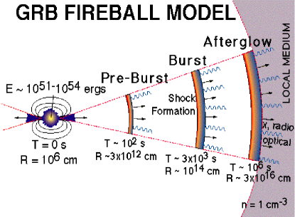
Figure 5: (a-b) Left panel (a) shows artists concept of the FB model with its internal/external shock formation and afterglow radiations in different energy bands and their time scales. Right panel (b) also shows artists concept of the CB model with its rotating accretion disk around the newly formed compact object in a result of core-collapse via supernova explosion and fall back matter (Dar 2006).

$\bullet$ Fireball (FB) model

FB model (Fig. 1.5a) was first proposed by Paczyński (1986) and Goodman (1986). But the present FB model is the vastly modified version of the old FB model (see, review articles of Zhang & Mészáros, 2004 and Piran, 2005). Most of scientific community believe that GRBs emit from the highly relativistic conical fireballs (Mészáros & Rees, 1992, Levinson & Eichler, 1993). These fireballs are produced by a rare class of massive energetic supernovae (SNe type Ic) explosions due to direct collapse of massive stars to black holes (Paczyński, 1988). In this case, observed GRB pulses are supposed to be produced by synchrotron emission due to the collisions between highly relativistic fireballs (conical shells), while GRB afterglow is also due to synchrotron radiation, but emits when the merged shells collide with the interstellar medium (ISM).

$\bullet$ Cannonball (CB) model

Present CB model (Dar & De Rújula, 2000, 2004) is modified version of the theorem introduced by De Rújula (1987) and his collaborator. In the CB model (Fig. 1.5b), it is assumed that long GRBs and their afterglows are produced by bipolar jets of cannonballs, which are believed to be produced due to the supernova explosions caused by the core collapse of ordinary stars. It is also believed that in the CB model, an accretion disk is formed around the newly borne compact object (like BH) by stellar materials near the surface of the collapsing core or by distant stellar mass fall into its passage (De Rújula, 1987).

6 Observational Data Analysis

The data analysis is essential to carry out work in observational astronomy. The observational study of astrophysical objects in any electromagnetic energy bands can be classified mainly in two types: $i)$ time series study/timing analysis and $ii)$ spectroscopic study/spectral analysis.

1 Timing Analysis

Timing analysis is the statistical study of measurements (equally) spaced over time. There can be various aims which include understanding the phenomenon represented in a single series, forecasting the future, and explaining the relationships between variables that change over time. The major feature of time-series data is that observations are not independent of previous observations. The pattern of serial dependence, or auto-correlation, must be accounted for in statistical analysis for inferences regarding the relationships between variables to be valid. In the astrophysical study timing analysis means the study of the astrophysical objects in time domain, i.e., how physical properties (luminosity, density, temperature, and chemical composition etc.) of the objects change with time. In our study of the X-ray properties of Sun and black holes, we concentrated on lightcurves, power density spectra, quasi-periodic oscillations, hardness softness diagrams for the timing analysis.

Light curve

Light curves (Fig 1.6a) are the graphs of the intensity or photon counts of astronomical objects as they change with time. The information contained in the lightcurve includes the timing of events, such as eclipses or pulses, and the amplitude of changes in the radiation received at Earth. For black holes the intensity of the light curve depends on the mass accretion rate (i.e. flow of matter from its companion objects).

Figure 6: (a-b) Left panel (a) shows GRO J1655-40 lightcurve (LC) and right panel (b) shows its Fourier transformed power density spectrum (PDS), observed on March 10, 2005. The LC shows periodicity, but oscillation frequency is not clear. From the PDS it is clear that LC has oscillation at 2.313 Hz. It also has a harmonic at frequency 4.599 Hz.

Each data point in a lightcurve is a photometric measurement, recorded at a particular time. These points represent measurements of the amount of radiation from the source received at the detector per second per area in a particular energy band.

Power Density Spectra

Power spectra (Fig 1.6b) tell us how the power is distributed at different frequencies. In the frequency domain, this is the square of the magnitude obtained by Fourier Transform. The power spectrum is computed either by a Fast Fourier Transform (FFT) algorithm or a direct Fourier algorithm on a lightcurve.

Quasi-Periodic Oscillations/Pulsations

In X-ray astronomy, quasi-periodic oscillations/pulsations (QPOs/QPPs) refer to the way the X-ray light from the vicinity of an astronomical object (white dwarf, neutron star or black hole) oscillates. The QPO phenomenon helps us to understand the innermost structure of accretion disks, nature of the accretion flow. Also from thorough study of this timing feature one can get an idea about the masses, radii and spin periods of the compact objects. A QPO is identified by performing a power spectrum on the lightcurve. A periodic pulsation appears in the power spectrum at exactly one frequency (a Dirac delta function), but on the other hand, a QPO appears as a broader peak of Lorentzian shape (see Fig. 16b).

There are many theories of the origin of QPOs, but it is generally accepted that the X-ray pulsation occurs due to an oscillating shock wave, generated by the infalling matter at the accretion disk of the compact object (Chakrabarti et. al. 2005, 2008a, Debnath et al. 2010a). According to the theory, the oscillation frequency is inversely proportional to the infall time scale of the matter from region of oscillation (i.e. shock location) to black hole. For the black hole candidates, observed QPO frequencies vary from mHZ to kHZ. The highest QPO frequency observed for any black hole candidate is 450 Hz (for GRO J1655-40). It showed QPO frequencies in the range of $0.01$ Hz - $450$ HZ (Remillard et. al. 1999, Strohmayer 2001, Debnath et. al. 2008a). For the Sun, people also have observed low frequency QPPs at the time of solar flares whose periods may vary from $10$s to $150$s (Young et al. 1961, Aschwanden 1987, Rao et. al. 2010a etc.).

As an alternative explanation for the origin of QPOs, some scientific people believe that the QPOs are caused by hot spots orbiting around a compact object. Since such a physical process is not sustainable for days after days, it is difficult to conceive that this is what is going on.

2 Spectral Analysis

Spectral analysis means the study of the astrophysical objects in energy domain. X-ray spectroscopy offers an important channel of information about our Universe. It is receiving increasing importance as X-ray astronomy has matured and technology is well developed. Now, we have the ability to make measurements not just of the X-ray continua, but of the discrete line features as well. From the analysis of the X-ray line spectra of an astrophysical object we can get an idea about the elemental composition and abundances, the temperature and electron temperature and density, magnetic field etc. Spectral analysis also tells us the physical processes occurring around (e.g. accretion disk around a compact object) or inside a celestial object.

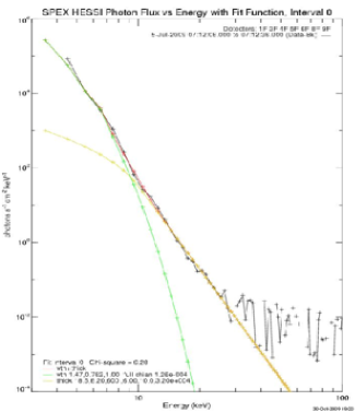
Figure 7: (a-b) Left panel (a) shows RXTE PCA 3 - 10 keV 2005 GRO J1655-40 outburst spectrum, observed on March 10, 2005 and the right panel (b) shows RHESSI observed spectrum of 5th July, 2009, C2.7 class solar flare.

A black hole spectrum contains mainly two components: thermal (black body nature) and non-thermal (power-law nature) (see, Fig. 1.7a). According to two component advective flow model (TCAF), thermal component is dominated by Keplerian photons (below, $\sim$ 10 keV), whereas the non-thermal component is dominated by sub-Keplerian photons (above $\sim 10$ keV). Based on the degree of importance of the black body and the power-law components black hole spectra can be divided into few classes. such as, hard, soft, intermediate etc.

Similarly, a solar spectrum also consists of two components: thermal and non-thermal. The thermal component consists of black body photons, where as the non-thermal component contains power-law photons due to bremsstrahlung or synchrotron emission (see Fig. 1.7b).

Chapter 1 Space Instruments, Data Acquisition and Analysis Procedure

The goal of my thesis is to study X-ray properties (spectral and timing properties) of Sun and some compact objects (mainly black hole candidates GRO J1655-40, GX 339-4 and gamma-ray bursts (GRBs)) of our Galaxy. These studies were done by analyzing the observational data from the space-borne X-ray telescopes. For studying X-ray properties of the Sun and gamma-ray bursts, we used X-ray data of the Indo-Russian collaborative RT-2 payloads (RT-2/S, RT-2/G and RT-2/CZT) and for the black hole study, NASA’s Rossi X-ray Timing Explorer (RXTE) satellite data were used. Apart from the X-ray data analysis, I participated in the development, test and evaluation and calibration of RT-2 payloads from its very initial stage to its final flight model stage. For the development of RT-2 systems, I also took part in some theoretical works such as: characterization of the detectors of RT-2/CZT imaging detectors using Fresnel Zone Plate (FZP) and Coded Aperture Mask (CAM) as coders for the hard X-ray imaging. This characterization was done by using Monte-Carlo simulation methods. In this Chapter, we will discuss about the descriptions of the RT-2 and the RXTE space instruments and their data acquisition, analysis procedures.

2.1 RT-2 Experiment: A mission for solar science

Sun occupies a special place in astrophysical studies as it can be more closely studied than any other star. Several dedicated satellites (RHESSI, SOHO, GOES etc.) have been launched to understand its behavior in a wide energy band of electromagnetic radiations. Even though its surface temperature is only $\sim$6000 K, it emits X-rays and $\gamma$-rays up to a few MeV. This is primarily because of rapid magnetic reconnection which produces energetic solar activities. Apart from the thermal electrons which obey Maxwell-Boltzmann distribution, the charged particles, especially electrons, are accelerated by shocks and acquire a non-thermal (power-law) distribution. These non-thermal electrons emit energetic synchrotron emissions. With time, the energy shifts from one wavelength to another. One of our goals is to understand the energy transport processes on the solar surface. It is due to plasma oscillations, or pinching or sausage instabilities in the magnetic field.

RT-2 (named after Röntgen) payload (Debnath et. al. 2008b, 2010b, Nandi et. al. 2009, 2010, Kotoch et. al. 2010, Sarkar et. al. 2010, Sreekumar et. al. 2010, Rao et al. 2010c) is a part of Russian Solar mission satellite named Coronas-Photon (Kotov et al. 2008, Nandi et al. 2009.). It was launched into $\sim$550 Km polar LEO (Low Earth Orbit) on 30^th January, 2009 from Plesetsk Cosmodrome, Russia. The mission is dedicated to study mainly the solar flares in a wide energy band of electromagnetic spectrum ranging from UV to high-energy $\gamma$-rays ($\sim$2000 MeV).

The main objective of the RT-2 Experiment is to study (i) time resolved hard X-ray spectra of solar flares, (ii) galactic and extra-galactic sources near the ecliptic plane, (iii) gamma ray bursts (GRBs) and (iv) diffused cosmic X-ray background, in a wide energy band of 15 keV to $\sim$ 1 MeV.

Figure 2.1: A realistic diagram of the CORONAS-PHOTON satellite.

The RT-2 payloads have been developed by Tata Institute of Fundamental Research (TIFR), Indian Centre for Space Physics (ICSP) in association with Vikram Sarabhai Space Centre (VSSC). I worked on the development of the RT-2 system as a team member, in laboratories of different Indian institutes, namely, VSSC (Thiruvananthapuram), SAC (Ahmedabad), PRL (Ahmedabad), TIFR (Mumbai) and ICSP (Kolkata).

2.2 RT-2 scientific payloads

RT-2 is an Indian Space Research Organization (ISRO) sponsored X-ray and low-energy $\gamma$-ray (up to 1 MeV) solar experiment in collaboration with MPhei, Russia. It consists of three scientific payloads (RT-2/S, RT-2/G & RT-2/CZT) and one master control electronic payload (RT-2/E). Both RT-2/S and RT-2/G payloads consist of identical NaI(Tl) and CsI(Na) scintillation crystals in a phoswich combination, having the same diameter ($116$ mm) but different thicknesses (Debnath et. al. 2010b). RT-2/CZT consists of solid state imaging detectors CZT (Cadmium Zinc Telluride) and CMOS (Complimentary Metal Oxide Semiconductor) (Kotoch et al. 2010). Main working energy range of RT-2/S & RT-2/G is of 15 - 100 keV (higher energy limit is extendable up to $\sim 1$ MeV) and for RT-CZT is of 20 - 100 keV.

All the three payloads are placed outside the hermetically sealed vessel of the satellite and co-aligned with the Sun pointing axis. The instruments have different viewing angles with Field of View (FOV) $4^{\circ}\times 4^{\circ}$ for RT-2/S, $6^{\circ}\times 6^{\circ}$ for RT-2/G and ranging from $6^{\prime}\times 6^{\prime}$ to $6^{\circ}\times 6^{\circ}$ for RT-2/CZT-CMOS.

Figure 2.2: Schematic diagram of RT-2 system (Sreekumar et al. 2010).

1 RT-2/S (RT-2/G) payload

RT-2/S and RT-2/G payloads consist of NaI(Tl) and CsI(Na) crystals mounted in a scintillator-phoswich assembly viewed by a photo-multiplier tube (PMT). The NaI crystal is of $3$ mm thickness and $116$ mm diameter is coupled with the CsI crystal of $25$ mm thick and of same diameter, to provide mechanical stability of the phoswich detector. These two crystals are optically coupled and hermetically sealed with an entrance window on NaI(Tl) side and a viewing glass window coupled to the PMT through an appropriate light guide on the CsI(Na) side. The NaI(Tl) crystal is sensitive to X-ray photons of $15-100$ keV, whereas CsI(Na) is effective for high energy X-rays/$\gamma$-rays of $30-1000$ keV as well as to charge particle background.

Both the detector assemblies sit behind a mechanical slat collimator surrounded by a uniform shield of Tantalum material and having different viewing angles of 4^∘ x 4^∘ (RT-2/S) and 6^∘ x 6^∘ (RT-2/G). As per design and scientific requirement, RT-2/S will work in the energy range of 15 keV to 100 keV, extendable up to 1 MeV, whereas aluminum filter is used to cut-off low energy photons ($\leq$ 20 keV) for RT-2/G payload.

Another important use of both the crystals in the Phoswich mode is for the background rejection. The light signal from the CsI(Na) crystal has a different scintillation decay time (650 ns) than that from the NaI(Tl) crystal (250 ns) and this distinction is used to eliminate non X-ray background in the NaI crystal. The charge particle background will be removed by the upper energy threshold. The Phoswich assembly is viewed by a $76.2$ mm diameter photomultiplier through a $10$ mm thick light guide.

Figure 2.3: A Schematic drawing of Phoswich assembly (NaI and CsI crystals) along with the PMT (Debnath et al. 2010b).

The interaction of X-ray photons of energy up to 100 keV with NaI and CsI crystals is fully dominated by the photo-electric process and thus absorbed radiation (secondary electron-hole pair absorbed by the impurities) converts into light photons (due to the decay of the excited impurities). These light photons eventually strike the photo-cathode of the PMT (Knoll 1999) (gain $\sim$10⁶) and converted into narrow electrical pulse whose magnitude (pulse height) is proportional to the energy of the incident radiation. Light outputs from NaI and CsI crystals have decay time scales of 250 ns and 650 ns respectively. Pulses from the detector (crystal) are amplified in a pre-amplifier and two post amplifiers (G1 and G2). Simultaneously, the pulse shape discriminator (PSD) is also measured as the width of the pulse. Output from one of the amplifier is selected based on the outputs from a Lower Level Discriminator (LLD) and an Upper Level Discriminator (ULD). If ULD is triggered, G2 is selected, otherwise G1 is selected. The output from the selected amplifier is digitized using an analog to digital converter (ADC). The ADC is 12 bits wide and has a typical conversion time of 10 $\mu$s.

The energy resolution (FWHM) of the scintillator Phoswich is expected to be $18\%$ at $60$ keV and the pulse height variation across the crystal will be less than $3\%$. The radioactive isotopes ²⁴¹Am (13.95, 17.74, 26.35 & 59.54 keV), ⁵⁷Co ($122$ keV), isotopes ²⁴¹Am ($13.95$, $17.74$, $20.8$, $26.35$ & $59.54$ keV), ⁵⁷Co ($122$ keV), ${}^{109}Cd$ ($22$ & $88$ keV) were used for laboratory calibration. The entire system

Electronics of both the instruments are identical, the only difference is that, RT-2/G has one Al sheet (thickness $\sim 2~{}mm$) above its collimator to increase its low energy cutoff. Both RT-2/S & RT-2/G detectors have 8 timing counters. Out of these 8 counters first 4 counters consist of G1-NaI(Tl) spectral information, next 2 counters consist of G1-CsI(Na) spectral information and the remaining 2 counters consist of G2 spectral information. The default spectral channel numbers of the counters and their calibrated energies are shown in Tab. 2.1.

Table 2.1: RT-2/S (RT-2/G) channel boundary (default) and energy ranges

Amplifiers	Counters	Channel ranges	Energy Ranges (keV)
		(default)	RT-2/S	RT-2/G
	C1	0 - 140	$<$ 13	$<$ 13
	C2	141 - 280	13 - 27	13 - 27
G1-NaI	C3	281 - 560	27 - 55	27 - 56
	C4	561 - 1023	55 - 102	56 - 104
	C5	0 - 256	$<$ 33	$<$ 34
G1-CsI	C6	257 - 1023	33 - 209	34 - 209
	C7	0 - 64	$<$ 48	$<$ 246
G2	C8	65 - 255	65 - 570	246 - 1000

2 RT-2/CZT payload

The RT-2/CZT payload consists of three CZT detector modules (OMS40G256, procured from Orbotech Medical Solutions Ltd., Israel) and one CMOS detector (RadEye-1, Rad-icon Imaging Corp., USA) arranged in a $2\times 2$ array. Each module of CZT detector consists of 256 individual pixels (detectors) of $2.5~{}mm\times 2.5~{}mm$, which are controlled by 2 ASICs and one CMOS detector consists of $512\times 512$ pixels of individual pixel dimension of $50\mu m$. The entire CZT-CMOS detector assembly sits behind a collimator with two different types of coding devices, namely Coded Aperture Mask (CAM) and Fresnel Zone Plate (FZP), surrounded by a uniform shield of Tantalum and has varying viewing angle of 6^′ - 6^∘. For the four detectors of the RT-2/CZT payload, four different combinations of imaging techniques has been used (Nandi et al. 2010).

RT-2/CZT payload is the only imaging device in the CORONAS-PHOTON mission to image the solar flares in hard X-rays of energy range from $20$ to $100$ keV. The effective area of 3 CZT modules is 48 cm² with an average energy resolution of 8$\%$ @60 keV (at 10^∘C). All three CZT detectors have the spectral information along with high resolution imaging capabilities. On the other hand, the CMOS detector has an effective area of 4.5 cm² with high resolution imaging capability only.

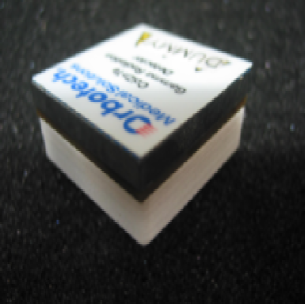
Figure 2.4: (a-b): Left panel (a) shows that the isometric view of a CZT Module used in RT-2/CZT of dimension 3.96 cm $\times$ 3.96 cm $\times$ 5 mm and right panel (b) shows the RedEye1 CMOS Detector, used in RT-2/CZT (Kotoch et al. 2010).

• Configuration 1 (CONFIG-1) contains CAM1 as coder and CZT1 as a detector. Spacing between CAM1 and CZT1 is $40~{}cm$, the angular resolution is $21.5~{}arcmin$ and FOV is 5.72^∘.

• Configuration 2 (CONFIG-2) contains CAM2 as coder and CZT2 as detector. The detector-coder spacing, angular resolution and FOV for this configuration is same as Configuration 1.

• Configuration 3 (CONFIG-3) contains dual FZP (FZP1) with diameter $3.0~{}cm$ as coder and CZT3 as detector. The spacing between the two zone plates is $32~{}cm$ and the angular resolution is $64~{}arcsec$. The FOV for this configuration is found to be $409~{}arcsec$ wide.

• Configuration 4 (CONFIG-4) is designed with dual FZP (FZP2) as shadow-caster of diameter $2.4~{}cm$ and a high spatial resolution pixilated CMOS as a detector. The spacing between two FZPs is $32~{}cm$, the angular resolution is around $54~{}arcsec$ and FOV is 4.29^∘.

In the following sub-section, we will discuss the physibility studies made for RT-2/CZT payload. In Nandi et al. (2010), we showed these results in details. Here I will discuss the Monte-Carlo simulation results made for only two combinations (CONFIG-1 & CONFIG-4) imaging detectors and coders out of four.

$\diamond$ Monte Carlo simulations for CAM and FZP

All the RT-2/CZT detectors along with coders will receive parallel rays of radiation as the sources are effectively at infinite distance when satellite is at its orbit. In general, it is difficult to make an experimental arrangement to keep source at infinite distance so that the shadow caster can receive parallel beam of X-rays. The only way we can verify that all the characteristics of the coders explained in above are true and examine their efficiency in reproducing exact replica of what they observe in their field of view is to simulate extensively all the required cases for all four configurations keeping all the parameters and environment intact (Nandi et al. 2010, also see, Chakrabarti et al. 2009b, 2009c, Palit et al. 2008, 2009).

Simulations using Monte Carlo method are done for every configuration and for all cases involving varying number of sources, with large off-axisness of source for the verification concerning FOVs and for closely placed sources to verify the mathematically obtained angular resolutions. The infalling photon number on the front coders (CAM1, CAM2, FZP1 and FZP2) for all four configurations is chosen to be 5$\times$$10^{5}$, while considering a single source. For double or multiple sources with varying intensity, photon numbers for the brightest source remain the same. The photon numbers for relatively lower intensity sources are mentioned in respective sections. This number is sufficient for hundred second (onboard accumulation time for each frame) data accumulation by the imager (4 different configuration for imaging in RT-2/CZT payload) from a $C$ class flare (and above) that occurred in the surface of the Sun.

Simulation results are interpreted based on the two-dimensional (2D) and three-dimensional (3D) representations of the reconstructed source positions and relative strength of the peaks. Source intensity variation in reconstructed image plane is plotted in arbitrary units. Detailed simulation results for CONFIG-1 & CONFIG-4 are presented in the following sub-sections.

$\bullet$ RT-2/CZT CONFIG-1 (CAM1 + CZT1):

CONFIG-1 consists of a single coder CAM (CAM1) and a CZT (CZT1) module and both are placed at $40~{}cm$ apart in the first quadrant of the collimator. CAM pattern for this configuration is shown in Fig. 2.5(a). A source position is generated at a position of $\theta$ = 42^∘ and $\phi$ = $1^{\circ}47^{\prime}$. The shadow of the CAM due to this source on detector plane is shown in Fig. 2.5(b). The shift of shadow pattern of the CAM from the central position codes the information on the position of source with respect to the central point in FOV. Reconstruction of the image (source position) from the CAM pattern is done in accordance with the method discussed above. In Fig. 2.5(c) and Fig. 2.5(d), we show the 2D and 3D views of the reconstructed source (image). In both Figs. of the reconstructed sky plane, the FOV is 5.72^∘ wide along in each sides. The reconstructed source position as we evaluated from Fig. 2.5(c), exactly matches with the actual source position assigned during simulation.

Figure 2.5: (a-d) shows, from left: (a) simulated picture of CAM1 pattern, (b) shadow pattern obtained in the CZT detector for CONFIG-1 for a single source, (c) 2D view of reconstructed sky plane, and (d) 3D picture of the source plane obtained by reconstruction (Nandi et al. 2010).

From Fig. 2.5(d), we get an estimation of the relation between the height of the peak of the reconstructed source and the actual intensity of the source.

In Fig. 2.6(a-c), we present the double source simulation results to verify the accuracy of the mathematically obtained angular resolution of the configuration containing CAM1 and CZT1. For this, we placed two sources at an angular separation of 21.5 arc minute from each other. The number of photons falling on the CAM from the brighter source is 5$\times$$10^{5}$ and that from the lighter one is 2.5$\times$$10^{5}$. In Fig. 2.6(a), we showed the shadow pattern obtained for two sources which are placed very close to each other. The reconstructed source (image) in 2D and 3D view of both the sources are shown in Fig. 2.6(b) and 2.6(c) . It can be seen from the Figs. that two sources are separated by one pixel between them. So the sources can be said to be just resolved.

Figure 2.6: (a) Shadow pattern obtained for two sources placed very closed to each other with CAM1 and CZT1 (left panel) configuration. (b) 2D view of reconstructed sky plane (middle panel). (c) 3D view of the source intensities obtained by reconstruction (right panel) (Nandi et al. 2010).

The CONFIG-1 and CONFIG-2 are identical as both configurations use CAM and CZT except that the CAM patterns are different in CAM1 and CAM2. Therefore, the FOV and angular resolution in both configuration are mathematically the same.

$\bullet$ RT-2/CZT CONFIG-4 (FZP2 + CMOS):

CONFIG-4 is the best possible configuration for imaging a hard X-ray source in terms of the achievable angular resolution. This configuration consists of dual FZP (FZP2) coder with a finest zone width of $0.0041$ cm and high position sensitive CMOS detector with the smallest pixel size of $0.005$ cm. The FZP coder is of negative cosine type. Inner zone radius of each zones is $0.1$ cm and the number of zones is $144$.

Figure 2.7: (a) Fringes obtained on a CMOS detector with a pair of zone plates as coded aperture (left). (b) 3D picture of the reconstructed source along with pseudo source which also appears in the reconstructed source plane. The central DC offset is chopped out (Nandi et al. 2010).

The Moire fringe pattern for the source with offset $\phi$ = 2.145^∘ is shown in Fig. 2.7(a). In Fig. 2.7(b), 3D view of the reconstructed source plane is shown along with the pseudo source (ghost source). Reconstructed source plane shows that the source is at extreme end of the FOV of the collimator, which confirms that the FOV is actually 4.29^∘ (twice the $\phi$ value).

Figure 2.8: (a) Fringes obtained (left) with a pair of sources at an angular distance from each other equal to the calculated angular resolution (54”) of the FZP2-CMOS combination. (b) 3D view of the reconstructed sources. To get a closer view, the part of the reconstructed plane containing the sources is zoomed, so that out of 600 pixels along each sides only 200 pixels are observed (Nandi et al. 2010).

The most important aspect of this configuration is the best possible angular resolution which could be around 54”. To verify the mathematically calculated angular resolution value, we simulate with two sources placed 54” apart and less than that. From simulation it is found that the sources which are placed less than 54” apart are not resolvable at all. In Fig. 2.8(a,b), we showed the fringe pattern and reconstructed the sky plane of two sources which are separated by 54”. The double pseudo source (ghost image) is also seen in the 3D view. Separation between the two closely placed sources are found to be equal to one detector pixel dimension.

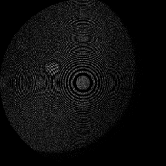
Figure 2.9: (a) Fringes obtained with a pairs of zone plates on CMOS detector for multiple sources (extended source) (left panel). (b) 2D view of the reconstructed sources (middle panel). (c) 3D view of reconstructed sources of the sky plane (right panel) (Nandi et al. 2010).

So far, we considered a point source to do the simulation. In principle, it is also possible to do simulation for extended sources. Simulation is done for the same configuration (CONFIG-4) with large number of point sources, which can be conveniently taken as an extended source. The fringe pattern along with 2D and 3D views of reconstructed sources are given in Fig. 2.9(a-c). The amplitude of individual reconstructed sources gives their relative intensities in the extended source distribution.

2.3 RT-2 data acquisition

RT-2/E contains master control electronics for the RT-2 system. It receives various operational commands from satellite ground communication system (SSRNI) and sends these commands to the RT-2 scientific payloads. It also sends ‘sec’ data send command to the detectors and receives data in every second. It also packetizes and compresses the RT-2 data and sends to the SSRNI. Finally satellite data can be downloaded from SSRNI, normally twice in a day. In the following sub-sections we will discuss about the RT-2 data structures and the modes of operations.

1 Data structure

Because the on-board memory size is 10MB, RT-2 data are sub-divided into two telemetry channels: 18 & 19, of each memory size 5MB. Channel 18 contains RT-2/S and RT-2/G spectral and timing data along with the health parameters of the payloads. Similarly channel 19 consists of RT-2/CZT spectral, timing and imaging data along with its health parameters.

$\bullet$ Data specifications of RT-2/S (RT-2/G):

Data specification for the two phoswich detector payloads RT-2/S & G are the same. Each photon event at RT-2/S (RT-2/G) detector generates 32 bit data: 12 bit ADC data, 1 bit for selecting G1/G2, 7 bit Pulse Shape (PS) and 12 bit Timing. These 32 bit event data along with the health parameters encoded in VCO, are packaged by FPGA and kept in a memory page. They contain a header block containing health parameters and counts, a spectrum block, a timing block with high time resolution counting and an event block. In detector Event mode maximum events that can be stored in memory per sec are 7360 events. The detailed data specifications for the RT-2/S and RT-2/G in Normal and Event mode (Sreekumar et. al, 2010, Debnath et al. 2010b) are given in the following Tab. 2.2.

Table 2.2: RT-2/S (RT-2/G) data specifications

VCO data: (2 bytes):
D15	D14-D12		D11-D0
Mode Id (0/1)	VCO Channel Numbers (0-7)		VCO Counts (values)
Scientific Data in NORMAL Mode:
	G1-NaI	2048 bytes	1024 spectral ch. $\times$ 1 word
Spectrum	G1-CsI	2048 bytes	1024 spectral ch. $\times$ 1 word
	G2	512 bytes	256 spectral ch. $\times$ 1 word
	PSD	256 bytes	128 spectral ch. $\times$ 1 word
TIMING	800 words	1600 bytes	8 ch. $\times$ 100 blocks $\times$ 1 word
COUNTERS	16 words	16 bytes	8 counters $\times$ 1 word
		Total 6480 bytes
Scientific Data in EVENT Mode: (4 bytes/event):
D20-D31	D13-D19	D12	D0-D11
Time	PSD	G1/G2 sel.	ADC

Detector data are send to RT-2/E for processing as ‘sec’ command is received. Header, spectral and timing blocks are sent in the Normal mode and header, event block are sent in the Event mode. These modes could be decided by ground command (Sreekumar et al. 2010).

$\bullet$ Data specifications of RT-2/CZT:

RT-2/CZT can be operated in two main detector modes: Event Mode and Normal Mode. Each photon event generates two words (32 bit) information. From these 32 bit data, we got header, spectral, image and timing data blocks. Data stored in the detector FPGA memory, are send to the RT-2/E at every second in response of ‘sec’ data send command. A CZT detector can accumulate maximum 4032 events. In Tab. 2.3, RT-2/CZT data specification (Kotoch et al. 2010) are given.

Table 2.3: RT-2/CZT data specifications

Event Mode: (4 bytes/event):
D31-D20	D19-D10	D9-D2	D1-D0
Time	ADC value	Pixel Id	Detector Id (0-2)
Normal Mode: CZT
Image	3072 words	1K words per CZT	4 ch. $\times$ 256 pixels $\times$ 1 word
Spectrum	1536 words	512 words per CZT
Timing	1200 words	400 words per CZT	4 ch. $\times$ 100 timing words
Counter	24 words	8 words per CZT	4 counters $\times$ 2 words
VCO	1 word	D15 (Mode Id: 0/1), D14-D12 (ch. No.), D11-D0 (counts)
Special	8 words	Telemetry, Temperature, Command sent, Data read against
		command, event number, CMOS line number, Calibration
		result identification word and Calibration status
Normal Mode: CMOS
Image	4096 words	(256 $\times$ 256) pixels $\times$ 1 bit
Sum	512 words	Vertical sum and horizontal sum (256 words each)

2 RT-2 operational modes

Depending upon different processor commands and detector commands, RT-2 system can work in different solar modes. Detectors can work mainly in two modes: NORMAL and EVENT (or Test). The processor can work in five different solar modes (which involve different data packets): Bad Mode, Test Mode, Debug Mode, Solar Quiet Mode (SQM), Solar Flare Mode (SFM).

RT-2 system mainly works on SQM and SFM. In both these operational modes, RT-2 detectors work on NORMAL mode. Only difference is that in SFM data comes from RT-2 scientific payloads (only RT-2/S & RT-2/G) to RT-2/E in 10 times faster rate.

Solar Quiet Mode - SQM (100 sec/frame)

This is the primary accumulation mode since the Sun is quiet in hard X-rays most of the time. In this mode, spectrum is obtained for every $100$ sec and count rates for every second in RT-2/S & RT-2/G. Similarly, from CZT detectors, the spectrum and the image are obtained in every $100$ sec and count rates are obtained in every second. From CMOS detectors, only image is obtained in every $100$ sec.

Solar Flare Mode - SFM (10 sec/frame)

The major science requirement for this experiment is the availability of high temporal and spectral resolution data during solar flares. Since such flares occur randomly, the onboard software has a built-in mechanism for checking the current count rate against the present thresholds to detect the flares. The flare search is carried out at every second. In this mode, data frame structure is identical to the solar quiet mode except that both the time resolutions are reduced by a factor of 10, i.e. in this mode count rates are every 0.1 sec and spectra are stored at every 10 sec. So, in this mode RT-2/S & RT-2/G data comes after every 10 sec, but RT-2/CZT data comes in every 100 sec since it does not have this operational mode.

Other than these two main operational modes, RT-2 system can also work in Test Mode (detectors work on EVENT mode, data comes in every second), Debug Mode (detectors work on NORMAL mode, but data comes in every one second). Apart from all these scientific functional modes, there have one safe mode (Bad Mode) and night mode (Shadow Mode). When the satellite enters into high flux region (SAA, North and South polar regions), satellite generates a BAD signal and depending on that signal, the whole RT-2 system operates into the BAD Mode. In this mode, data comes in every $100$ sec. Shadow Mode is activated when the Sun is out of satellite’s field of view, i.e., during the instruments night time and also at solar occultation time. In this mode data comes mainly in every $100$ sec.

2.4 RT-2 data analysis procedure

The scientific data from the three RT-2 detector payloads is stored temporarily in the memory of RT-2/E. After proper packetization, data is compressed with the onboard software (Sreekumar et al., 2010). The compressed data is transferred to the satellite system (SSRNI) for down-link to the ground station as soon as the telecommand is received.

RT-2 scientific and satellite telemetry data normally downloaded to the ground station twice a day. Scientific telemetry data contains scientific timing, spectral and imaging (only for RT-2/CZT) data for all the three detectors. Similarly satellite telemetry data contain every $4$ sec monitored satellite health status, i.e., physical parameters (temperature, memory, Flare, Corona, HV status etc). RT-2 data comes from the satellite via two telemetry channels: 18 & 19. The allotted memory size for each channel is $5MB$. The Channel 18 contains RT-2/S & G data, where as 19 channel contains RT-2/CZT data.

RT-2 scientific data which comes from the satellite are compressed. So, before analyzing scientific data we need to run the task ‘decomp’ to decompress the downloaded compressed data, which could be 10 to 12 times more in size than the compressed data depending on the mode of operation. This decompressed data is analyzed using a software written in LabVIEW. These LabVIEW programs can analyse and save health parameters, timing, spectral and image data of the three detectors in ASCII formatted files.

Figure 2.10: (a-c) Left, middle and right panels show (a) RT-2/S, (b) RT-2/G and RT-2/CZT lightcurves for the 4048 CORONAS-PHOTON orbit data, observed on $26^{th}$ October, 2009.

1 Timing Data Analysis

RT-2/S & RT-2/G has 8 timing counters, bear different energy bands of spectral channel/energy informations. Default pre-launch counter energy ranges for RT-2/S & RT-2/G have been given in Tab. 2.1. For SQM and SFM we get respectively 1 sec and 0.1 sec time resolution for RT-2/S & RT-2/G detectors. Figure 2.10(a-b) shows RT-2/S & RT-2/G lightcurves of the flight data of orbit 4048. The observation date of the data is $26^{th}$ October, 2009. RT-2/S & RT-2/G channels 1-5 have detected a B1.0 class solar flare on this data at 07:52:00 UT, are shown in Figure.

RT-2/CZT has 12 timing counters (4 for each CZT detectors). Counters 1-4 are allocated for CZT module 1, 5-8 are for CZT 2 and rest 9-12 are for CZT 3. Each counter corresponds to some specific channels of CZT1, CZT2 & CZT3 spectra. Default channel ranges for counters 1, 5 & 9 are: 0 - 64 channels; for counters 2, 6 & 10 are: 65 - 128 channels; for counters 3, 7 & 11 are: 129 - 192 channels; and for counters 4, 8 & 12 are: 193 - 511 channels. Fig. 2.5 (c) shows RT-2/CZT lightcurve of the satellite orbit 4048 (observed on $26^{th}$ October, 2009). Due to the noise at the CZT pixels, we have not been able to detect the solar flare observed by RT-2/S & RT-2/G in RT-2/CZT lightcurve data.

Figure 2.11: (A-B) Top panel four spectra are of RT-2/S detector: (a) PSD spectrum, (b) G1-NaI(Tl) spectrum, (c) G1-CsI(Na) spectrum and (d) G2 spectrum and lower panel four spectra are of RT-2/G. Onboard calibration source peak of ⁵⁷Co (122 keV) is detected at G1-CsI & G2 spectra and $I^{121}$ decay peak (58 keV) is detected at G1-NaI spectra.

2 Spectral Data Analysis

Both RT-2/S and RT-2/G have 3 energy spectra (G1-NaI, G1-CsI & G2) and one PSD spectrum. PSD spectrum shows the pulse shape of the events from NaI and CsI crystals and the channel value at the ‘valley’ of the PSD spectrum is applied to separate the NaI & CsI photon counts, which are registered in G1 amplifier as NaI and CsI spectra. PSD spectrum is of total 128 channels. Pulse Shape (PS) cut value for RT-2/S is 26 channel and for RT-2/G is 28 channel. The spectra of G1-NaI & G1-CsI has 1024 channel informations, whereas G2 has spectral information in 256 Channel. Energy calibrated G1-NaI spectrum is capable of detecting photons up to $\sim$ 100 keV. G1-CsI & G2 spectra are capable of detecting high energy photons up to 1 MeV. The strong peak in the G1-NaI spectrum is of emission from ²⁴¹Am radio-active source (59.5 keV). Other strong peaks in the G1-CsI and G2 spectra are of emission from ⁵⁷Co radio-active source (122 keV), which is used as onboard calibration source. The energy resolution of both the instruments (RT-2/S & RT-2/G) are found to be around $18.72\%$ (RT-2/S) and $18.36\%$ (RT-2/G) at 60 keV.

Figure 2.12: (a-c) Top panel (a) shows CZT module 2 spectrum of the satellite orbit 441, observed on $28^{th}$ February, 2009. Bottom left panel (b) shows the CZT 2 image and right panel (c) shows CMOS background image for the same satellite orbit. In the images, Y & X axes indicate pixel numbers of the detector modules.

In Fig. 2.11(a-b), the spectra of PSD, G1-NaI, G1-CsI & G2 for RT-2/S and RT-2/G detectors of the satellite orbit 2051 (observed on $15^{th}$ June, 2009) are plotted. From the PSD spectra it is clear that PS cutoff value of RT-2/G1-NaI(Tl) & G1-CsI(Na) spectra for RT-2/S & RT-2/G detectors are at 26 & 28 channels respectively.

RT-2/CZT payload consists of three solid state imaging CZT detectors and one CMOS detector. All the three CZT detectors (CZT1, CZT2 & CZT3) can acquire both solar spectral and image informations but the CMOS has only imaging capability. The energy range for the CZT detectors are $20-100$ keV. RT-2/CZT spectrum for CZT 2 module is shown in Fig. 2.12(a), for the in-flight RT-2 data of the satellite orbit 441 (first RT-2/CZT high voltage switch ON orbit, was observed on $28^{th}$ February, 2009).

3 Image Data Analysis

As mentioned before, all the three CZT detectors and the CMOS detector of the RT-2/CZT payload receive imaging information. In Fig. 2.12(b), CZT module 2 image of $28^{th}$ February, 2009, orbit 441 is plotted. In Fig. 2.12(c), CMOS background image has been plotted. Image of the CZT detector contains $16\times 16$ pixel matrix (total 256 pixels) of each pixel size $2.5~{}mm$ and CMOS detector contains $256\times 256$ pixel matrix of pixel size $50~{}\mu m$.

2.5 RXTE: A mission for compact object study

My thesis work for the observational black holes study is based on Rossi X-ray Timing Explorer (RXTE) data. RXTE is a NASA’s astronomy mission satellite, was launched from Cape Canaveral on 30 December, 1995, on a Delta rocket. This mission gives a huge bust in our understanding about the astrophysical objects. This satellite was launched to study the most luminous sources of our Galaxy (i.e. X-ray binaries), Active Galactic Nucleies (AGNs), quasars, pulsars etc. Major advantage of this satellite over previous X-ray instruments is due to its unparalleled detector characteristics and wide energy range (2 - 200 keV). RXTE detectors have unique capability of acquiring X-ray photons with $\mu$s time resolution over a wide energy band, which is quite able to probe temperature, magnetic fields and other fundamental physical properties close to the observed sources (mostly compact objects) as well as the geometry of the systems, nature and characteristics of the compact object itself (e.g., masses, spin rotation periods and size of the compact objects etc.). RXTE consists of three main scientific instruments: the All-Sky Monitor (ASM) (Levine et al. 1996), the Proportional Counter Array (PCA) (Jahoda et al. 1996), the High Energy X-Ray Timing Experiment (HEXTE) (Rothschild et al. 1998).

RXTE is a polar satellite which orbits the earth at an altitude of $\sim$580 km with an inclination angle 23^∘ and a period of $\sim$100 min. Therefore it passes over the South Atlantic Anomaly (SAA) region in 6 of its daily 14 - 15 orbits for each time duration of 10-20 min. During SAA region time, all instruments are put into the safe mode to protect them against the highly charge particle SAA flux.

The satellite already has worked more than 13 years and still it is working. More than 1700 scientific papers have published on the basis of RXTE data, near about 100 Ph.D thesis have been submitted on the basis of the study of RXTE data. Also it has discovered more than 50 astrophysical X-ray sources.

2.6 Brief discussion about RXTE scientific payloads

NASA astronomy satellite RXTE consists of three scientific payloads: ASM, PCA and HEXTE. In this Section we will discuss briefly about the configurations of these three instruments.

1 All-Sky Monitor (ASM)

The ASM (Fig. 2.13) of RXTE has been designed to monitor the sky in 1.5 - 2.0 keV energy band. The ASM consists of three Scanning Shadow Cameras (SSCs). A motorized drive assembly is used to rotate these SSCs for viewing different parts of the sky. Each SSC contains a Position Sensitive Proportional Counter (PSPC) system which views the sky through coded aperture mask. The mask is of a thin Al sheet of 15 transparent (open) and 16 opaque (closed) matrix elements of equal dimensions. Each PSPC contains 8 resistive carbon-coated quartz fiber anodes, each end of which is connected to a dedicated electronic measurement chain.

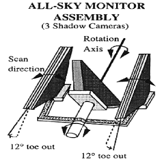
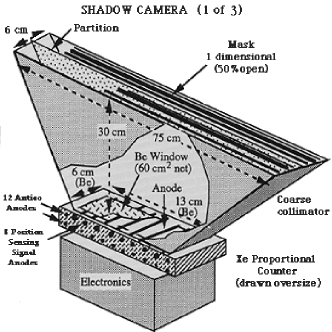
Figure 2.13: (a-b): Left panel (a) shows the ASM assembly with 3 shadow cameras and right panel (b) shows the detailed cross-sectional view of one shadow camera (courtesy: NASA).

Observing X-ray source intensity and direction, measurements are derived from the displacements and strengths of the shadow patterns cast by the X-ray sources with the camera’s field of view (FOV). Each camera has FOV of $6^{\circ}\times 90^{\circ}$ FWHM and detection sensitivity up to 30 mCrab (1 Crab = 75.5 SSC cts/sec). The X-ray events detected by ASM are normally processed on-board by two ASM Event Analyzers (EAs) in the Experiment Data System (EDS). Typically, a source is observed $5-10$ times a day, and the full coverage is obtained in a series of 90 sec stationary exposures known as ‘dwells’. The ASM also provides the unequally sampled data in one-day average from a number (typically $5-10$) of individual ASM dwells. ASM has proved to be a unique instrument on-board RXTE due to its fascinating first-results or quick look capability, such as detection of a new transient in the sky, state change of known sources and quasi-periodic or highly flux variations in a longer time scale etc.

The ASM archival data for the observed sources are available at the NASA site (http://xte.mit.edu/ASM_lc.html). Data are available in three different energy bands: a-band (1.5 - 3.0 keV), b-band (3 - 5 keV) and c-band (5 - 12 keV).

2 Proportional Counter Array (PCA)

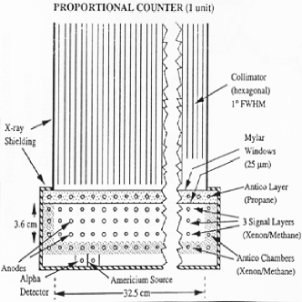
Figure 2.14: (a-b): Left panel (a) shows the PCA assembly with five PCUs and right panel (b) shows the detailed cross-sectional view of one PCU (courtesy: NASA).

The PCA (Fig. 2.14) of RXTE has been designed mainly to study timing properties of bright galactic sources and also for faint extra-galactic sources in 2 - 60 keV X-ray energy band with unique time resolution of 1 $\mu$sec. PCA consists of 5 Proportional Counter array Units (PCUs). Each detector has an effective area of $\sim~{}1300~{}cm^{2}$. PCA has a good energy resolution of $18\%$ @ 6 keV.

Each PCU consists of a hexagonal beryllium copper made collimator with $1^{\circ}$ FWHM FOV and two gas-filled chambers mounted on top of each other. The first chamber is filled with propane (veto layer) and it protects the other from background radiations. The second chamber is filled with a mixture of Xenon/Methane (90/10) gas and it is the main X-ray detector for each PCU. This chamber contains 4 layers of anode grids separated by cathode wires (per grid 20 anodes are present). The upper 3 layers, each splitted into two (left and right), are used for X-ray detection. The X-rays impacting on a Xenon atom generate a cascade of electrons and they are collected by the high voltage anode. The higher the X-ray photon energy, the more electrons are generated, and thus the higher the electron pulse-amplitude. The anodes in the grid of the last layer serve as a discriminator i.e., veto layer for charged particles entering through the detector walls.

My thesis work for the observational study of black hole candidates are mainly on the basis of this PCA data analysis results. The PCA archival public data for the observed sources are available at the NASA site (http://heasarc.gsfc.nasa.gov/cgi-bin/xte/all_too.pl).

3 High Energy X-Ray Timing Experiment (HEXTE)

Figure 2.15: HEXTE cluster assembly with eight ($2\times 4$) phoswich detectors, each cluster contains 4 phoswich detectors are shown (courtesy: NASA).

The HEXTE (Fig. 2.15) of RXTE has been designed to study the timing and the spectral properties of bright sources in hard X-ray regime of 15 - 250 keV. The HEXTE consists of 2 independent clusters (A or 0 and B or 1) of detectors, whereas each cluster contain 4 NaI(Tl)/CsI(Na) phoswich scintillation counters sharing a common 1^∘ FWHM FOV. Total detection area of the 8 detectors is 1600 $cm^{2}$. Each detector covers the whole energy range of 15 - 250 keV with an average energy resolution of 15.4% FWHM @ 60 keV. The cluster orientation of the HEXTE instrument permits effective immunity to systematic background variations through the use of continuous gain control, chopping of the source signal and anti-coincident shielding for the charge particle events.

The HEXTE has provided important spectral information in the high energy band, but the nominal count rates (e.g., 289 counts/sec for the Crab) and low sensitivity (1 Crab = 360 count/sec per HEXTE cluster) limit its use for timing studies. HEXTE archival data can be downloaded from the same NASA site of PCA data.

2.7 RXTE data analysis procedure

RXTE archival public data for all observed astrophysical sources are available at NASA RXTE TOO page (http://heasarc.gsfc.nasa.gov/cgi-bin/xte/all_too.pl). All the data are in fits format. Data analysis FTOOLS (HEASoft) software package is also available at NASA site (http://heasarc.gsfc.nasa.gov/docs/software/lheasoft).

Satellite on-board processor which processes ASM, PCA and HEXTE event data is called Experiment Data System (EDS). EDS consists of 8 Event Analyzers (EAs): six for PCA & HEXTE data system and two for ASM, winch can process incoming event data into 8 different modes. Two preset EAs of PCA data are:

1. the Standard-1 data mode provides data in the energy range of $2-60$ keV with a time resolution of 0.125 sec and no energy resolution since all 256 channels are combined into one channel,

2. the Standard-2 data mode provides data in the same energy range of $2-60$ keV with a time resolution of 16 sec and high spectral resolution (the pulse height is recorded in 129 channels covering the $2-60$ keV energy range, although maximum energy limit changes from one Epoch to another Epoch).

Other four EAs for PCA data can be set by the principal investigator (PI) of the observation or by the RXTE ground operation staffs. In general most used EAs’ are ‘Event’,‘Binned’ and ‘Single-Bit’. In Event mode, data is transferred to the ground station as a time series of unevenly spaced events described by arrival time, pulse height, PCU ID etc. and this mode has different configurations like: Generic event ($E\_62us\_32M\_36\_1s$ or $E\_125us\_64M\_0\_1s$), Good Xenon (Good_Xenon1_2s), Transparent. In a Binned mode, the actual photon arrival time is lost. The events are binned with respect to time, photon energy and detector number. The Generic binned ($B\_8ms\_16A\_0\_35\_H$), Standard-1 and Standard-2 are different configurations of Binned data mode. Data of Single-Bit mode consists of a stream of ones and zeros representing detector events and clock ticks (set the time resolution). The generic Single-Bit configurations are designated with a character string beginning with SB ($SB\_500us\_50\_249\_2s$) and it has the same format as that of the Binned mode with higher time resolution between the two events.

The data analysis is to be done for data obtained in ’good time’ of the detector. We need to make a good time intervals (GTI) file. The GTI file is created with ftool task maketime. The ftool task xtefilt is needed to create the filter file, automatically consulting the appropriate housekeeping files. This task requires the Observation Id no., FITS Master Index (FMI) file and a file listing the Application IDs (appids) as input. For normal science binned data ftools task saextrct is used to create lightcurve (.lc) and for the same purpose task seextrct is needed for event mode data. To run these commands pca SAA information file is needed to pass. Also for the spectral study creating spectral file (.pha), it is needed to run task saextrct on Standard-2 data. For the spectral study, the background file in very important. For creating the background file from raw data task runpcabackest is required to run. For this purpose pca background calibration file of data epoch is needed to pass.

Similarly for HEXTE data, the ftools task hxtback is needed to create the background file. Since HEXTE instrument is designed to study the high energy data, the dead time correction is essential. For that purpose, ftools task hxtdead is required to run. Other commands are the same as for PCA, such as making GTI files (using maketime), creating lightcurves (.lc) and spectral (.pha) files (using saextrct) etc.

2.8 Models used in fittings of RXTE timing and spectral data

Data reduction and analysis for the black hole candidates were carried out with the FTOOLS version of HEADAS-6.1.1 software and XSPEC version 12.3.0. For the detailed timing and spectral analysis we used FTOOLS inbuilt package models. In the following sub-sections we will discuss about nature of the fitting models, which we used for the temporal and spectral studies of black hole X-ray binaries.

1 Timing analysis models

After making the lightcurves for the source data using saextrct or seextrct commands we load (or plot) the lightcurves into the “PLT” (pgplot) mode. Then we can fit them using standard FTOOLS XRONOS package models or user defined local models. In general for the timing analysis, we fit power density spectra using CONS (frequency independent constant factor), POWR (due to non-thermal power-law emissions), LORE (Lorentzian line profile) and GAUS (Gaussian line profile). The best fit results are obtained by using the least square fit technique. To find $\chi^{2}$ fit value, we need to run command ‘stat’ and to find model parameters’ uncertainties, we need to run ‘uncer’ command (for e.g., ‘uncer 1’ to see uncertainty for fitted parameter 1). Also to calculate $\pm$ error values for the fitted model parameters, we use “fit err” task, which gives us the $90\%$ confidence range of any fitted parameter. Now, we will discuss about the above fitted models in details.

$\bullet$ CONS

The model $``CONS"$ represents nothing but an energy independent multiplicative constant factor, needs for improving fit statistics. It can also be defined as power-law model (POWR) with ‘zero’ slope value.

$\bullet$ POWR

This model represents the power-law nature of the radiating photon distribution. This power-law nature of the emitted photons occurs mainly due to the non-thermal radiative processes. The $``POWR"$ model uses two parameters: power-law slope index ($\alpha$) and normalization (PN). The power-law distribution can be defined by the following simple relation:

$$A(\nu)=K~{}\nu^{-\alpha},$$

where $\alpha$ is the dimensionless power-law slope index and $K$ is the power-law normalization factor PN.

$\bullet$ LORE

This model indicates the Lorentzian line profile. In our analysis, we used this model to find QPO centroid frequencies. It uses three parameters: line frequency (LC), line full width at half maximum (FWHM) and line normalization (LN). The $``LORE"$ model profile with frequency ($\nu$) can be defined as:

$$A(\nu)=\frac{LN}{(1+[\frac{2(\nu-LC)}{LW}]^{2})}.$$

The sharpness of the QPO peak is calculated by the quality (Q) factor, which is defined as

$$Q=\frac{\nu_{0}}{FWHM}=\frac{\nu_{0}}{2\Delta}=\frac{LC}{LW},$$

where $\nu_{0}$ is the QPO centroid frequency and $\Delta$ is the half width at half maximum.

Also rms amplitude of the Lorentzian fit profile can be calculated by the relation:

$$rms~{}amplitude=100(\sqrt{I/{\rm mean~{}count~{}rate}}),$$

where $I$ (=$\pi*LN*LW/2$) is the integral of the Lorentzian.

$\bullet$ GAUS

The model $``GAUS"$ represents Gaussian line profile. It has also three model parameters: line frequency (GC), line full width (GW) and line normalization (GN). This model profile with frequency ($\nu$) can also be defined as

$$A(\nu)=GN~{}exp[-0.5(\frac{\nu-GC}{GW})^{2}]=GN~{}exp[-Z^{2}/2],$$

where $Z=(\nu-GC)/GW$. Also we can calculate the integral value of this Gaussian model profile by the factor $\sqrt{2\pi}*GN*GW$.

2 Spectral analysis models

In the same manner we extract spectral .pha files from the source and corresponding background “Standard-2” mode data files using FTOOLS task saextrct. These pha files are first rebinned using command rbnpha and then loaded in the XSPEC along with energy response file. Now this loaded spectrum can be fitted by using default XSPEC models or by user defined local models. In general for the spectral data fittings, we fit energy spectra for the black hole candidates by using wabs (photo-electric absorption due to intermediate media between source and observer), diskbb (black body model modified for the black hole accretion disk), powerlaw (non-thermal power-law distribution), gauss (Gaussian peak for line emissions) and compST (Sunyaev-Titarchuk Comptonization model). The best-fit can be obtained by using appropriate combination of models and by observing the value of the reduced $\chi^{2}$, which can be defined as

$$\chi^{2}=\sum_{i=1}^{N}(\frac{\Delta_{i}}{\sigma_{i}})^{2}=(\frac{\Delta_{1}}{\sigma_{1}})^{2}+(\frac{\Delta_{2}}{\sigma_{2}})^{2}+\ldots+(\frac{\Delta_{N}}{\sigma_{N}})^{2},$$

where $\Delta$s are the difference between observed and theoretical values, $\sigma$s are the size of the error bars. The reduced $\chi^{2}$ value is calculated by the relation $\chi^{2}_{red}$ = $\chi^{2}$/$DOF$, where Degrees of Freedom ($DOF$) = $N-P$; $N$ is the number of data points and $P$ is the number of free model parameters required to fit the data. For the best-fit, this $\chi^{2}_{red}$ value should be $\sim 1$. Sometimes to obtain the best-fit results we need to add extra model component and that addition of extra model can be verified via F-test by using ftest command, which requires to pass $\chi^{2}_{red}$ values. In the following sub-sections we will discuss about the nature of the above mentioned fitting models.

$\bullet$ wabs

The $``wabs"$ model, uses photo-electric absorptions using Wisconsin cross-sections (Morrison & McCammon 1983). Energetic radiations from the astrophysical sources get absorbed by the intermediate media between observers and sources. This absorption mainly occurs due to the photo-electric process. This model uses only one fitting parameter and can be defined by the following simple relation:

$$M(E)=exp[{-{n_{H}}~{}\sigma(E)}],$$

where $\sigma(E)$ is the photo-electric Wisconsin cross-section (not including Thomson Scattering) and fitted parameter ($n_{H}$) is equivalent to the hydrogen column density in units of $10^{22}~{}atoms~{}cm^{-2}$.

$\bullet$ diskbb

The $``diskbb"$ model represents the multi-colour black body spectrum comes from the accretion disk. This model is known as the disk black body model. It basically represents the modified version of the black body model spectrum which is radiated from the black hole accretion disks. The Eqn. 1.2 of the introductory Chapter 1, is the governing equation of this model and there we also briefly discussed about this model. This model uses two parameters: disk black body temperature ($T_{in}$) at inner disk radius in keV and disk black body normalization. This normalization factor is the value of $(r_{in}~{}in~{}km/D~{}in~{}10kpc)^{2}cos\theta$, where $r_{in}$ is the apparent inner disk radius, $D$ is the distance of the source, and $\theta$ is the disk inclination angle (see, Mitsuda et al. 1984, Makishima et al. 1986 and Kubota et al. 1998). So, from the model fitting we can easily calculate the inner disk radius and temperature.

$\bullet$ powerlaw

This model represents the power-law nature of the non-thermal radiating nature of the accretion processes. This may occur by the processes non-thermal inverse Comptonization, synchrotron or cyclotron emissions (discussed in the introductory Chapter 1). This model uses two parameters: power-law photon index ($\Gamma$) and power-law normalization ($K$). The power-law distribution spectrum can be defined as:

$$A(E)=K~{}E^{-\Gamma},$$

where $\Gamma$ is the dimensionless power-law photon index and $K$ is the power-law normalization factor. This $\Gamma$ value increases as the spectrum becomes softer. For the hard state spectra this $\Gamma$ value is less than $\sim 2$ and for the soft state this value is above $\sim 3$.

$\bullet$ gauss

This model indicates the simple Gaussian line profile. We use this model to fit Iron emission line $\sim 6.5~{}keV$. This model uses three parameters: line energy in keV, line width in keV and normalization in unit of $photons~{}cm^{-2}~{}s^{-1}$. The $gauss$ model spectral distribution can be defined as:

$$A(E)=K\frac{1}{\sigma\sqrt{2\pi}}exp[-(E-E_{l})^{2}/2\sigma^{2}],$$

where $E_{l}$ is the parameter 1 (line energy) in keV, $\sigma$ is the parameter 2 (line width) in keV and $K$ is the parameter 3, normalization factor. This $K$ represents the value of the total number of photons in $cm^{-2}~{}s^{-1}$ at the line.

$\bullet$ compST

This $compST$ model is the Sunyaev-Titarchuk (1980) Comptonization model. This model indicates the presence of the Comptonized cool photon cloud on the disk. This model also uses three parameters: Compton cloud temperature ($kT$) in keV, optical depth ($\tau$), and normalization. The normalization represents the value of the function $Nf/4\pi d^{2}$, where $N$ is the total number of photons from the source, $d$ is the distance to the source, and $f$ is the factor $z(z+3)y^{z}/\Gamma(2z+4)\Gamma(z)$. In the factor $f$; $z$ is the spectral index, $y$ is the injected photon energy in units of temperature, and $\Gamma$ is the incomplete gamma function.

Chapter 2 Solar Science using RT-2

RT-2 instruments onboard CORONAS-PHOTON mission satellite was launched on $30^{th}$ of January, 2010 into a $\sim$550 Km polar LEO orbit mainly for the detailed timing and spectral study of the Sun in soft and hard X-ray regime. So far, RT-2 has detected a few hard X-ray solar flares and gamma-ray bursts. In this Chapter, we will discuss about the results obtained due to the solar flares.

3.1 Solar flares and physics behind its origin

A flare is defined as a sudden, rapid, and intense variation of brightness in the timing data of an astrophysical object. A solar flare occurs when the magnetic energy that has built up in the solar atmosphere is suddenly released. Radiation is emitted across the entire electromagnetic spectrum, from radio waves to high energy X-rays, $\gamma$-rays. The first solar flare recorded in astronomical literature was on September 1, 1859. Two scientists, Richard C. Carrington and Richard Hodgson, were independently observing sunspots at the same time, when they were viewing a large flare in white light.

Solar flares are the most powerful emissions in the entire solar system and they release energies of $10^{32}$ to $10^{33}$ ergs in $100$ to $1000$ seconds. It is also found that during the flare, electrons are accelerated up to $10-100$ keV using a significant fraction of this energy budget.

There are typically three stages of a solar flare. First is the precursor stage, where the release of magnetic energy is triggered. Soft X-ray emission is detected in this stage. In the second impulsive stage, protons and electrons are accelerated to energies exceeding 1 MeV. During the impulsive stage, radio waves, hard X-rays, and $\gamma$-rays are emitted. The gradual build up and decay of soft X-rays can be detected in the third, decay stage. The duration of these stages can be as short as few seconds or as long as an hour.

Solar flares extend out to the layer of the Sun called the corona. The corona is the outermost atmosphere of the Sun, consisting of highly rarefied gas. Inside a flare, the temperature typically reaches 10-20 million degrees Kelvin, and can be as high as 100 million degree Kelvin. The corona is visible in soft X-rays. In general corona is not uniformly bright, but concentrated around the solar equator in the loop-shaped features. These bright loops are located within and connect areas of strong magnetic filed called active regions. Sunspots are located within these active regions. Solar flares are also occur in these active regions.

The frequency of the flares coincides with the Sun’s 11 year cycle. When the solar cycle is at a minimum, active regions are small and rare and few solar flares are detected. The increase in number occurs as the Sun approaches the maximum part of its cycle. The Sun is expected to reach maximum activity period in the year 2011.

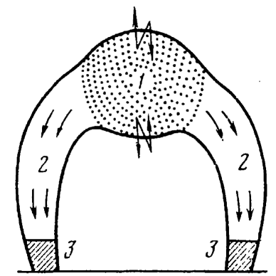
Figure 3.1: A model for hard X-ray emissions and quasi-periodic pulsations during solar flare in the coronal loop. $1)$ is the region of the initial energy release, where fast magnetic-reconnection process occurs and a fraction of hard X-ray emission comes out, $2)$s are regions of modulated fast electron streams, $3)$s are the regions, from where maximum hard X-ray radiations are emitted (Zaitsev & Stepanov 1982).

In most observed solar flares, the hard X-ray radiation comes from the footpoints of the magnetic loops (regions marked as $3$ in Fig. 3.1) (Krucker et al. 2008, Duijveman et al. 1982), presumably as the the thick-target bremsstrahlung of fast electrons stopped in the cold and collisionally dense chromosphere (Brown 1971, Hudson 1972). Recent RHESSI observations have revealed a new class of events in which the hard X-ray emission comes predominantly from the coronal flare loop (region marked as $1$ in Fig. 3.1) itself, with little or no emission from the footpoints (Veroing & Brown 2004, Sui et al. 2004, Goff et al. 2005).

According to Krucker et al. (2008), the coronal hard X-ray sources can be divided into two classes. The first class concentrates on properties of hard X-ray sources produced only by transport effects (e.g., binary collisions, magnetic mirroring etc.), leaves coronal acceleration as a “black box”. This theory is known as the classical thick-target theory (Brown 1971, Hudson 1972). Alternatively, one can include self-consistent particle acceleration processes.

X-ray spectra provide a way to distinguish the radiation emitted by hot, thermal electrons from that emitted by accelerated, non-thermal electrons. The shape of the X-ray spectrum emitted by thermal electrons is distinct from that emitted by the non-thermal electrons. The radiation observed at soft X-ray energies is typically from thermal plasma with a temperature on the order of 10 - 30 million degrees Kelvin.Recent RHESSI observational results (Hudford et al. 2002, Battaglia & Benz 2006) tell us that the spectrum consists of a combination of thermal bremsstrahlung and spectral lines (e.g., Fe, O, Mg etc.) from the elements in the hot plasma. The hard x-ray spectrum is dominated by bremsstrahlung from the accelerated electrons and, at the lower hard x-ray energies, thermal bremsstrahlung from plasma with a temperature above around 30 million degrees Kelvin. Also, one may observe soft-hard-soft spectral evolution at the impulsive phase of coronal footpoint sources (Krucker et al. 2008). This spectral evolution strongly suggests the presence of the acceleration mechanism rather than to the coronal transport.

In some rare occasions, quasi-periodic pulsations (QPPs) can be observed during the solar flare. There are theoretical models in literature for the QPP, out of them two models are most popular: $1)$ plasma model, in which the modulation of emitted radiation is related to periodic regimes of plasma instabilities, and $2)$ magneto-hydrodynamic (MHD) model, in which the emitted radiation is modulated by the source (magnetic tube) MHD oscillations (Zaitsev et al. 1984).

From RHESSI observations, it has been established that the particle acceleration and the energy release process (Lin et al., 2003) are linked together. Therefore, it is a unique opportunity to investigate the energetic solar flares with RT-2/S & RT-2/G (Debnath et al. 2010) mainly in the energy range $15$ to $150$ keV in Phoswich mode and $\sim 100$ keV to $1$ MeV in spectroscopic mode during the next $24^{th}$ solar cycle. At the same time, it is also possible to image the hard X-ray solar flares with the RT-2/CZT payload, which has been designed to work in the energy range of $20-150$ keV (Kotoch et al. 2010). It has very good spectral as well as spatial resolutions.

3.2 Solar flares observed with RT-2

After its successful launch on January 30, 2009, RT-2 has detected several hard X-ray solar flares. Both RT-2/S & RT-2/G instruments of the RT-2 Experiment, onboard CORONAS-PHOTON mission satellite detected the GOES C2.7 class solar flare on 5th July, 2009 (Rao et al., 2010). In this solar flare, we have observed hard X-ray Quasi-Periodic Pulsations (QPPs) of time period $\sim 12$ seconds. We have also detected a series of low energetic solar flares during the recent solar eruptions from $22^{nd}$ October, 2009 to $2^{nd}$ November, 2009. These flares were detected mostly in the low energy X-ray band ($<$ 25 keV). In this week, we observed two solar flares on $26^{th}$ October, 2009. On $26^{th}$ October, at 07:52:00 UT, a B1.0 class solar flare was detected by RT-2/S and at 22:48:00 UT, a C1.3 class solar flare was detected by the both RT-2/S & RT-2/G detectors. In the following sub-Sections we will discuss the results obtained from the first detected, $5^{th}$ July, 2009 solar flare (in details) and some preliminary results of the later (October 26, 2009) observed low energetic solar flares.

1 Hard X-ray QPPs observed in $5^{th}$ July, 2009 solar flare

The C2.7 class solar flare was detected by the both phoswich detectors (RT-2/S & RT-2/G) of the RT-2 experiment. The flare was observed mainly in the hard X-ray energy band ranging from 15 - 59 keV (see Fig. 3.2a). During the flare time both of the RT-2/S and RT-2/G detectors were in Solar Quiet Mode (frames per 100 sec (spectra per 100 sec and timing per sec) and detectors are in NORMAL Mode). Light curves of RT-2/S & RT-2/G in the energy range below 35 keV shows multiple peaks, with some signature of periodic pulses. These periodic nature in the lightcurves motivate us to make deeper analysis in timing as well as spectral domain. The strongest peak count rate for RT-2/S is $\sim 325$ counts/sec and that of RT-2/G is $\sim 90$ counts/sec. We carry out the Fourier analysis of these lightcurves and found hard X-ray Quasi-Periodic Pulsations (QPPs) of period $12$ seconds. We augmented these results using the publicly available data from the $RHESSI$ satellite. Also, we made spectral analysis and measured the spectral parameters.

Figure 3.2: (a,b) Left panel (a) indicates RT-2/S and RT-2/G lightcurves in different energy band (marked). In the energy range below 35 keV RT-2/S shows indication of a stronger flare than what is observed in RT-2/G. This is because RT-2/G detector has a $2$ mm Aluminium filter above its collimator and is effective only above $\sim$ 25 keV. The data bin size is 1 s and T₀ is UT 07:08:50 on July 5, 2009. Right panel (b) indicates GOES and RHESSI lightcurves of the flare. Top panel: GOES lightcurves in the bands 1 - 8 $\AA$ (3.1 - 24.8 keV) and 0.5 - 4 $\AA$ (1.6 - 12.4 keV) (from top) with the time resolution of 1 minute. Bottom panel: RHESSI light curves in the energy bands: 6-12 keV, 3-6 keV and 12-25 keV (from top). Bin size is 4 seconds and T₀ is UT 07:08:50 on 5th July, 2009 (Rao et al. 2010).

The satellite was at high latitudes at the beginning of the observations and the background rates slowly stabilized when the satellite approached towards low background equatorial region. Since the detectors (RT-2/S & RT-2/G) use the Phoswich technique, the changing background has negligible impact on the $<$ 35 keV lightcurves. For example, the background rate during the first $200$ second of observation (in this energy band) is 36.6$\pm$0.4 s^-1 and it is 36.4$\pm$0.4 s^-1 towards the end of observation.

The RT-2/G detector has an Aluminium window to block X-rays below $\sim$25 keV (Chapter 2). The lightcurves from RT-2/S and RT-2/G detectors in two channels are shown in Fig. 3.2(a). The bin size is 1 second and T₀ is UT 07:08:50 on 2009 July 5. Quasi-periodic pulsations are clearly seen in the lightcurve. We define the rising phase of the flare as between 125 to 225 s (07:10:55 to 07:12:35) and the falling phase as between 225 s to 325 s (07:12:35 to 07:14:15).

GOES and RHESSI Observations

The data from GOES and RHESSI satellites are shown in Fig. 3.2(b). According to RHESSI, the flare is dominated mainly in the X-ray band of 12-25 keV range which correspond to channel 2 data of our RT-2/S, RT-2/G payloads. The flare started at 07:08:28 UT and ended at 07:21:32 UT with peak at 07:12:22 UT on July 5, 2009. Total duration of the flare is 784 sec, average counts is $\sim 84$ and sum counts is $113983$. This is the first major hard X-ray (above 12 keV range) observed by RHESSI in 2009 and also after the launch of our CORONAS-PHOTON Satellite. Fig. 3.2(b) clearly shows that both in RHESSI and GOES hard X-ray photons dominate over soft X-ray photons. Also from the GOES lightcurves we can classify the flare as of C2.7 class.

Quasi-Periodic Pulsations

Quasi-Periodic Pulsations (QPPs) during solar flares have been observed for many years (Young et al. 1961) and their periodicities vary from milliseconds to several seconds. The fast QPPs of millisecond durations are generally attributed to some wave-particle interactions (Aschwanden 1987). On the other hand, the long period QPPs (periodicity $>$ 10 s) observed in the microwave emission of solar flares are also seen in hard X-rays (Nakariakov et al. 2003) and they could be resulting from some MHD oscillations in the source region or due to modulation of electron acceleration and injection mechanisms. Jakimiec and Tomczak (2009) have investigated QPPs in about 50 flares using $Yohkoh$ and $BATSE$ hard X-ray data and have derived a correlation between the QPP periods (ranging from 10 s to 150 s) and sizes of loop-top sources. They conclude that the hard X-ray oscillations are confined to the loop-top sources and the observations are described with a model of oscillating magnetic traps. Fleishman et al. (2008) have made a detailed analysis of the 2003 June 15 solar flare (GOES X1.3 class) and detected hard X-ray (based on $RHESSI$ data) and microwave oscillations with periods ranging from 10s to 20s. They, however, conclude that QPPs are associated with quasi-periodic acceleration and injection of electrons.

Since the basic cause of QPPs have implications for particle acceleration mechanism, it is important to investigate QPPs at diverse source intensities. we observe QPP in the C2.7 solar flare, detected by RT-2 on 2009 July 5 (Rao et al. 2010). In the next sub-sections spectral and temporal characteristics of the flare will be discussed.

Timing Analysis

In the lightcurves of RT-2/S and RT-2/G (Fig. 3.2a), we observe multiple peaks, which motivate us to make Fourier transformed power density spectra and find periodicities. To find the modulation power and the periodicities, we follow the method used in Fleishman et al. (2008). If $C(t)$ is the count rate at time $t$, the normalized modulation is

$$S(t)=\frac{C(t)-<C(t)>}{<C(t)>}$$

where $<C(t)>$ is the running average taken over a number of bins, which is 20 s in our case. The modulation power over a period of time is equal to the average of S²(t) and the square root of modulation power is the modulation amplitude (see, Fleishman et al. 2008).

Figure 3.3: (a,b) Left panel (a) shows RT-2/S low energy lightcurves with normalized modulation in the four energy bands, shown in Fig. 3.2(a) and right panel (b) shows the power spectra of these lightcurves (Rao et al. 2010).

In Fig. 3.3(a), we plotted the normalized modulation along with the count rates. The top panel shows the count rates in the RT-2/S 20 – 35 keV range and the successive panels downwards show the normalized modulation for RT-2/S 20 - 35 keV, 35 - 59 keV and similarly for RT-2/G, respectively. To estimate the errors in the modulation power, we calculated the modulation power in the background regions for a period of $100$ sec, and the RMS deviation is deemed as the error in the measured values. The background subtracted modulation powers, for 4 second integration time, are given in Tab. 3.1, for the rising and falling phase of the flare, respectively.

In Fig. 3.3(b), we showed the Fourier transform of the normalized modulation, for RT-2/S 20 - 35 keV total lightcurve (top panel) and rising phase (35 - 59 keV) of the flare (second panel from top). The third and fourth panels show similar power spectra for the RT-2/G lightcurves. The periods of the highest peaks in the power spectra are also shown in Tab. 3.1.

Table 3.1: Modulation amplitudes and QPP Periods of the solar flare

Observation	Rising Phase		Falling Phase
	Amp. (%)	Period (sec)	Amp. (%)	Period (sec)
RT-2/S 20 – 35 keV	13.5$\pm$0.4	15.3$\pm$0.1	5.2$\pm$0.4	12.2$\pm$0.2
(2nd peak)	- -	11.9$\pm$0.2	- -	- -
RT-2/S 35 – 59 keV	4.6$\pm$2.8	- -	$<$ 5.6	- -
RT-2/G 25 – 35 keV	6.6$\pm$0.4	12.1$\pm$0.2	$<$ 0.8	15.6$\pm$0.3
(2nd peak)	- -	15.5$\pm$0.3	- -	- -

Spectral Analysis

Solar hard X-ray spectrum is of isothermal and power-law type, can be fitted with the combination of isothermal and double-power-law (or broken power-law) models (Lin et al. 2003, Krucker et al. 2008). At the same time, the black hole X-ray spectrum is a combination of black body and power-law types (This will be discussed in the following Chapters in detail.). In this Section, we will discuss the model fitted spectrum of the 5th July, 2009 solar flare.

Before going to fit RT-2/S & G spectra, we generated appropriate response matrices for the detectors which were generated using FTOOLS ‘genrsp’ task. For the channel - energy calibration we used the background line at 58 keV (due to ¹²¹I decay) of the on-board calibration source ⁵⁷Co. The values of energy resolution function measured during the ground calibration and the effective areas from the known geometrical properties of the detectors are used for response matrix generation. Background spectrum obtained away from the solar flare is used. The XSPEC tool of the $ftools$ package is used for spectral fitting. The deconvolved 20 - 35 keV spectra are shown in Fig. 3.4 (a) for RT-2/S (filled circles) and RT-2/G (open circles). The spectrum is very steep and it is best fitted by a simple bremsstrahlung function of energy 3.43$\pm$0.30 keV. This model is shown as a dashed line in the Figure.

Figure 3.4: (a-b) Left panel shows (a) the deconvolved spectra from RT-2/S (filled circles) and RT-2/G (open circles) along with a simple bremsstrahlung spectrum (dashed line) and right panel shows (b) the RHESSI photon energy spectra during the rising phase of the flare (07:11:40 to 07:12:30). The two component thin and thick target bremsstrahlung model is also shown in the Figure (Rao et al. 2010).

We also made spectral study of the flare using RHESSI archival data. Fig. 3.4(b) shows the background subtracted and spatially integrated 3 - 100 keV spectra from RHESSI observations for the rising phase and the falling phase of the flare. We used the standard RHESSI software of Solar SoftWare (SSW) for the creation of spectrum and the RHESSI OSPEX package is used for the spectral fitting of the count spectra.

The RHESSI spectrum was fitted with a two component power-law model, consisting of an optically thin thermal bremsstrahlung radiation function, parametrized by the plasma temperature $kT$ and the emission measure (EM) and a thick target bremsstrahlung, characterized by the electron flux and the power law index ($\Gamma$) of the electron distribution function below the break energy. It can be seen that the 20 - 30 keV RHESSI spectrum agrees quite closely with the RT-2 data.

2 Low energy solar flare detected on $26^{th}$ October, 2009

A series of low energy solar flares was detected by the RT-2 instruments during the recent solar eruptions from $22^{nd}$ October, 2009 to $2^{nd}$ November, 2009. These observed flares are mostly in the low energy X-ray band ($<$ 25 keV). During this week, RT-2 has detected two solar flares on $26^{th}$ October, 2009.

(a) A very weak flare of B1.0 class was detected by RT-2/S detector at 07:52:00 UT. The flare was so weak that it was detected only by the channels 1 & 2 of the RT-2/S detector (see Fig. 3.5). RT-2/G signature is very weak (signal to noise ratio $\sim$ 1). This is because RT-2/G detector has an extra $2~{}mm$ Aluminium sheet (for low-energy cutoff) above its collimator (Chapter 2). During the flare time, both of our RT-2 phoswich instruments (RT-2/S & RT-2/G) were at Solar Quiet Mode. So, we got a highest time resolution of 1 sec.

Figure 3.5: (a-b) Left panel shows (a) the RT-2/S lightcurves for channels 1-4 and right panel shows (b) the RT-2/G lightcurves for channels 1-4 of the B1.0 class solar flare, was detected at 07:52:00 UT on $26^{th}$ October, 2009. Channels 1 & 2 of RT-2/S show the clear detection of the flare.

(b) A flare of C1.3 class was also detected by the both phoswich detectors of the RT-2 experiment (RT-2/S and RT-2/G) at 22:48:00 UT on $26^{th}$ October, 2009. At the low energy bands (below 25 keV), flare was detected by the energy channels 1 & 2 of the RT-2/S detector and by the channel 1 & 5 of the RT-2/G detector (see Fig. 3.6). Here also during the flare time both the instruments were at Solar Quiet Mode.

Figure 3.6: (a-b) Left panel shows (a) the RT-2/S lightcurves for channels 1-4 and right panel shows (b) the RT-2/G lightcurves for channels 1-4 of the C1.3 class solar flare, was detected at 22:48:00 UT on $26^{th}$ October, 2009. Channels 1 & 2 of RT-2/S and Channel 1 & 5 of RT-2/G show the clear detection of the flare.

Detailed analysis of the above mentioned solar flares and other flares are continuing. The detailed timing and spectral analysis results will be published in near future (Debnath et al. 2010d).

Chapter 3 GRO J1655-40: An Outbursting Galactic Black Hole Candidate

The Galactic black hole candidates are the most fascinating objects to study in X-rays, as these sources undergo peculiar timing and spectral changes during their transient as well as the persistent phases. GRO J1655-40 is a well studied Galactic black hole candidate. The soft X-ray transient GRO J1655-40 was first observed by BATSE onboard CGRO on 27th July, 1994 (Zhang et al. 1994). This source was extensively observed with RXTE during its outburst of 1996-1997 and also in 2005 (Fig. 4.1). In 1996-97 outburst, it showed a very complex timing and spectral behaviour and was X-ray active at least for $16$ months. We made a detailed timing and spectral studies of the full 2005 outburst using publicly available RXTE archival data (Debnath et al. 2008a, Chakrabarti et al. 2005, 2006a, 2008a). These analysis results will be discussed in this Chapter.

GRO J1655-40, an enigmatic Low Mass X-ray Binary (LMXB) system is located at $(l,b)=(344.98^{\circ},2.45^{\circ})$ (Bailyn et. al. 1995) with R.A.=$16^{h}54^{m}00^{s}$ and Dec.= $-39^{\circ}50^{m}45^{s}$. Its mass (M = $7.02\pm 0.22~{}M_{\odot}$, Orosz & Bailyn 1997) distance (D = $3.2\pm 0.2$ kpc, Hjellming & Rupen 1995), and inclination angle ($\theta=69.5^{\circ}\pm 0.1^{\circ}$, Orosz & Bailyn 1997) are well determined. The mass of its companion star is = $2.3~{}M_{\odot}$ (Bailyn et. al. 1995). GRO J1655-40 may also showed signatures of the ejection of the superluminal radio jet (Tingay et. al. 1995, Hjellming & Rupen 1995). The maximum speed of the jet was found to be $\sim 0.37c$. Recent VLT-UVES spectroscopic observations suggest that the distance to the source is $\leq 1.7$ kpc (Foellmi et. al., 2006) with a secondary star of spectral type of F6IV, making it one of the closest known black hole candidates.

4.1 Major results obtained from the past outbursts

The transient black hole candidate GRO J1655-40 showed two well studied X-ray outbursts in 1996-97 and 2005. These two large outbursts were quiet extensively observed by RXTE satellite. In the following sub-sections, we will briefly discuss the major results obtained so far from the above two outbursts. In particular, we studied the detailed timing and spectral properties of the 2005 outburst.

1 1996-97 GRO J1655-40 outburst

The transient Galactic black hole GRO J1655-40 showed a major outburst in the years 1996-97 for a total duration of $\sim$ 16 months (see, Fig. 4.1A). The ASM lightcurve of the outburst shows a double peak profile and it is quite different from other black hole candidates. During the first peak in May, 1996, the source showed a strong flaring activity with non-thermal emission, whereas during the second peak in August, 1997, the source spectrum was softer and thermal, except near the end of the outburst when its spectrum was hard (Sobczak et. al. 1999). At least three distinct spectral states, namely, very high state, high/soft state and low/hard state (Sobczak et al. 1999) have been reported. The luminosity variation of the outburst was of fast rise and exponential decay (Chen et. al. 1997). Investigation of X-ray timing properties of GRO J1655-40 during the 1996-97 outburst revealed QPOs varying from $0.1$ Hz to $300$ Hz (Remillard et. al. 1999). Two very important discoveries were found there: one is the superluminal radio jet (Tingay et. al. 1995, Hjellming & Rupen 1995) and the other is the existence of very high QPO frequencies ($300$ & $450$ Hz) (Remillard et. al. 1999, Strohmayer 2001).

Figure 4.1: (A,B) Left panel (A) shows the 1996-97 GRO J1655-40 outburst and right panel (B) shows the 2005 outburst. In both the Figures, (a) 2-12 keV ASM lightcurve and (b) hardness ratio (5-12 keV vs. 2-5 keV count ratio) as a function of the Modified Julian Day (MJD) of the event are plotted. In the right panel, the vertical dashed lines indicate the spectral transition of states and dotted horizontal points are our analyse days (Fig.B: Debnath et al. 2008a).

2 2005 GRO J1655-40 outburst

After remaining ‘dormant’ for almost eight years, GRO J1655-40 showed a renewed X-ray activity in the late February 2005 (Markwardt & Swank 2005, Chakrabarti, Nandi, Debnath et al. 2005, Shaposhnikov et al. 2007, Chakrabarti, Debnath, Nandi & Pal 2008a, Debnath, Chakrabarti, Nandi & Mandal 2008a, Debnath et al. 2008c). The source remained active in X-rays for the next $260$ days and during this period it was extensively observed with the RXTE satellite (see Fig. 4.1B).

In our communication (Debnath et al. 2008a), we presented a detailed analysis of the RXTE (ASM and PCA) archival data of 122 days which spread over the full period of the outburst and present the results for both the timing & the spectral properties of GRO J1655-40 during this outburst phase, which reveal several very important aspects of the nature of the transient accretion process around a black hole.

From the lightcurves, hardness/softness diagrams, spectral slopes and most importantly the variation of the QPO frequency, one can come up with a very comprehensive picture of what might be happening when such an outburst takes place. In the entire outburst phase, we identified four spectral states characterized by the presence or absence of a soft multi-color disk black body component at low energy and the power-law component at higher energies above $\sim 10$ keV. The four identified states are termed as the hard, soft, very-soft and intermediate states. During the total outburst we observed the transitions in the sequence: hard $\rightarrow$ soft/very soft $\rightarrow$ intermediate $\rightarrow$ hard. In each of these spectral states, we carried out detailed timing and spectral analysis and find QPO frequencies.

In the previous communications (Chakrabarti et al. 2005, Chakrabarti et al. 2008a), the evolution of the QPO frequencies with time was shown in the initial and final outburst stages. The rapid variation in QPO frequencies was explained by using an oscillating and propagating shock.

Shaposnikov et. al. (2007) also carried out a multi-wavelength study for the early stage (beginning with 21st of February, 2005) of the outburst of GRO J1655-40 for a total of 25 days of data using instruments like RXTE & INTEGRAL for X-rays, VLA for radio study and ROSTE & SMARTS for optical region. On the basis of their multi-wavelength campaign they classified the spectral states of the observed period in four spectral states, namely, low-hard, hard intermediate, soft intermediate, high-soft. After correlating X-ray and radio fluxes they concluded that the physical origins of the radio emission and the X-ray emission are not the same. The evidence of a closer coupling between the power-law component and QPO as also observed by Vignarca et. al. (2003) is totally consistent with the shock propagation model of Chakrabarti et al. (2005, 2008a) as the shock does not propagate in the disk as they mentioned, but through the sub-Keplerian flow which surrounds the disk (e.g., Chakrabarti & Titarchuk, 1995).

Our study, on the other hand, covers 122 days of the observational data spreading over the full period of the outburst. On the basis of the results of RXTE data, we classified the total outburst in a slightly different way with four distinct spectral states. Furthermore, we thoroughly studied the QPO behaviour. We got QPOs in a total of $67$ observations out of a total of $150$ observations. We also studied the photon count variation in different energy bands for different spectral states via hardness and softness intensity diagrams. We identify the energy band in which QPOs are predominantly seen. We show spectral components and their flux variations. We claim that two components of the flow, namely, the Keplerian (disk) and the sub-Keplerian (halo) are necessary to explain the mass accretion dynamics. We theoretically estimate the disk and the halo rates from spectral fits of several observations.

In the following Sections, we will discuss the major results obtained from our study in the both timing and spectral domains.

4.2 Timing Analysis

Timing analysis of 2005 GRO J16555-40 outburst depends on the data analysis results on the publicly available observational data from the RXTE instruments, the All Sky Monitor (ASM) and the Proportional Counter Array (PCA) covering the entire eight months of the outburst. Our analysis covers from the 25^th of February, 2005 (Modified Julian Day (MJD) = 53426) to 16^th of October, 2005 (MJD = 53659). The ASM data has four energy bands corresponding to $2-3$ keV, $3-5$ keV, $5-12$ keV and $2-12$ keV. PCA contains five proportional counter units (PCUs 0-4). We used only PCU 2 data for both the timing and spectral analysis due to its reliability and it is on for $\sim 100\%$ of the good time. Data reduction and analysis were carried out with the FTOOLS version of HEADAS-6.1.1 software and XSPEC version 12.3.0.

We used the PCU2 data from the Event mode ($E\_125us\_64M\_0\_1s$) and Science Array mode ($B\_8ms\_16A\_0\_35\_H$) data for the timing analysis. Our timing analysis is mainly to study the lightcurves with hardness and softness variations and the power density spectra (PDS) of each data. Out of these observations, we find QPOs in a total of $67$ observations made in $43$ days. Timing analysis results are discussed in the following sub-sections.

1 ASM Light Curve

We extracted and analyzed the ASM (Levine et al. 1998) data of different energy bands for the entire observations. In Fig. 4.1(B), the total 2-12 keV ASM lightcurve (counts/sec) and the ASM hardness ratio (ratio of the photon count rates in 5-12 keV and 2-5 keV bands) are plotted. The origin of the time axis is MJD 53420 ($19^{th}$ February, 2005), which is six days before the initial rise of the X-ray intensity. The hardness ratio variation distinctly reflects the state transitions. The hard to soft transition takes place on the $13^{th}$ of March, 2005 (MJD = 53442), the soft to intermediate transition on the $16^{th}$ of May, 2005 (MJD = 53506), and the intermediate to hard transition takes place on the $12^{th}$ of September, 2005 (MJD = 53625). These are marked on the plot, using vertical dashed lines. However, the local changes in the spectral features of different states are not evident from this plot. This leads us to conduct a robust spectral analysis using the PCA data and the results are discussed in the next sub-sections.

2 Hardness-Intensity Diagram

We extracted and analyzed the PCA (Jahoda et al., 1996) data of the full outburst from February 25, 2005 (MJD = 53426) to October 16, 2005 (MJD = 53659). Figure 4.2(a-b), shows RXTE ASM and PCA hardness-intensity diagrams (HIDs) respectively. In Fig. 4.2(a), the ASM 2-12 keV count rates for the full period of 2005 GRO J1655-40 outburst are plotted against hardness ratio of 5-12 keV and 2-5 keV ASM photon counts. In the same way, in Fig. 4.2(b), the PCA 3-20 keV count rate of the 2005 outburst against X-ray color (PCA count ratio between 6-20 keV and 3-6 keV energy bands) are plotted. It is evident that the pre and post-outburst phases tend to appear and disappear from the low count region having harder spectrum. In this GRO J1655-40 outburst, the transition occurs from the spectral states hard $\rightarrow$ soft (very soft) $\rightarrow$ intermediate $\rightarrow$ hard. It is observed that the rapid changes in the hardness ratio occurs only in the hard states, whereas in the soft and intermediate states the hardness ratio changes very slowly. Both rising & falling arms of the diagram corresponds to the hard state. In both the cases, we found the presence of QPOs.

Figure 4.2: (a-b) The Hardness Intensity Diagrams (HIDs) observed with RXTE ASM & PCA. For ASM HID, count rates are plotted (in y-axis) in the energy range of 2-12 keV and in the x-axis hardness ratio of the photon counts between 5-12 and 2-5 keV are plotted. Similarly in the PCA HID, the y-axis represents the PCA count rates in 3-20 keV energy band and the x-axis represents the hardness ratio between the count rates of the energy bands of 6-20 keV and 3-6 keV bands, are plotted (Fig.b: Debnath et al. 2008a).

In the first phase of the hard state from the 25^th of February, 2005 (MJD = 53426) to the 12^th of March, 2005 (MJD = 53441), we found QPOs from $34$ mHz to $17.78$ Hz. The observed QPO frequencies were found to be increased monotonically with time (day) from 0.082 Hz to 17.78 Hz (on the first day another QPO at $34$ mHz was also seen). This QPO frequency rise was observed up to $\sim 15$ days from the initial observed day. This was because, after 12^th of March 2005, the Keplerian component became dominant over the sub-Keplerian component and could been able to cool down the disk, which in fact stopped the shock oscillations and observed QPO signatures. So, we observed hard to soft state transition on 13^th March, 2005 (MJD = 53442). The soft state started from the March 13, 2005 and continued till 15^th of May, 2005 (MJD = 53505). In this region no QPO was observed. The intermediate state was seen from the 16^th of May, 2005 (MJD = 53506) to 11^th of September, 2005 (MJD = 53624). Interestingly, in this state, we observed QPOs only for $8$ days, from 16^th of May, 2005 (MJD = 53506) to 20^th of May, 2005 (MJD = 53510) and from 25^th of May, 2005 (MJD = 53515) to 27^th of May, 2005 (MJD = 53517). In between, for four days we observed no signature of QPOs. The QPO frequencies varied were from $13.17$ Hz to $19.04$ Hz. In the PDS, we also found one broad QPO bump at frequencies near $7$ Hz. The final hard state observed was from the 12^th September, 2005 (MJD = 53625) to October 16, 2005 (MJD = 53659). The QPOs of $0.023$ Hz to $20.20$ Hz were observed in this state. If we follow one of the QPO frequencies (of sharp peak and high “Q” value), we found it to decrease monotonically from $13.14$ Hz to $0.034$ Hz within $20$ days.

3 Light curves and Hardness, Softness diagrams

For the detailed study of the photon count variations over the outburst, we extracted 2 - 15 keV (0-35 Channels) PCA lightcurves with a time bin of 1 sec also studied both the hardness and softness ratio variations. Also for the power density spectra (PDS), we extracted PCA lightcurves with 0.01 sec time bins. These lightcurves were extracted using FTOOLS task “saextrct” on Science data and tasks “sefilter” & “seextrct” on Event mode data. To plot the lightcurves “fplot” task was used. The hardness and the softness ratio diagrams were made by extracting lightcurves for three energy bands: $A:0-8$ channels ($2-4$ keV), $B:9-35$ channels ($4-15$ keV) and $C:36-138$ channels ($15-60$ keV). A hardness diagram is the plot between $C/A$ vs. $B/A$ while the softness diagram is the plot between $B/C$ vs. $A/C$. Our motivation of splitting the energies in this way stems from the fact that the Keplerian disk primarily emits at a low energy ($\lower 2.15277pt\hbox{$\;\buildrel<\over{\sim}\;$}4$ Kev) for the mass of the black hole, we were interested in. Thus, $A$ would be emitted mostly from the Keplerian component. The component $B$ would be emitted from the region where the moderate thermal Comptonization of the Keplerian photons took place. The component $C$ would be emitted from the region which was definitely depleted or enhanced during state transitions as it was represented at the higher energy side of the pivotal energy [$\sim 15$ keV] in the spectrum. Thus, these diagrams were not directly connected to the spectral states - - rather, they were connected to the geometry, i.e. the number of soft photons produced by the Keplerian disk ($\sim A$) and the seed photons intercepted by the ‘Compton cloud’ [$\sim(B+C)$] and the number of scatterings they undergo ($\sim B$ or $\sim C$).

Figure 4.3: (a-d):In the lower panel, 2 - 15 keV (0-35 Channels) PCA lightcurve and in the upper panel the hardness and softness diagrams are plotted. In hardness diagrams, the dashed horizontal ($B=A$), vertical ($C=A$) and the dotted line ($B=C$) are for reference purpose. In softness diagram they represent $C=A$, $B=C$ and $A=B$ respectively. Observation dates are: (left to right) (a) on 10th of March, 2005 (Obs ID:90704040100) at the initial rising hard state phase, (b) on 20th March, 2005 (Obs ID:91702-01-08-00) at the Soft/Very soft state, (c) on 17th of May, 2005 (Obs ID:91702015700) at the intermediate state, and (d) on 17th of September, 2005 (Obs ID:91702017900) at falling hard state phase of the outburst (Debnath et al. 2008a).

From Figs. 4.3(a-d) and 5.4 (a), we obtain an approximate idea on the evolution of high energy and low energy seed photons i.e. about the supply the Keplerian (disk) and the Sub-Keplerian (halo) matter/photon rates.

(a) Hard State in the rising phase:

Figure 4.3(a) shows initial hard state lightcurve and hardness-softness intensity diagrams of 10th March, 2005. From the Figure, it is clear that $B>A>C$. So, here the intensity of the intermediate energy photons is stronger than low and hard X-ray photons. Here we observed QPOs of frequencies 2.313 & 4.59 Hz. During the full initial hard state observations, we observed QPOs with monotonically increasing frequencies. But just after three days (on 13th of March) of the present observation, QPO vanished and the spectrum became softer and moved towards the soft/very soft state.

(b) Soft/Very soft State:

Figure 4.3(b) shows soft/very soft state lightcurve and hardness-softness intensity diagrams of 20th March, 2005, when the source was in the soft state. From the Figure, we can interpret that $B>A>>C$. The $C$ component is further reduced while $A$ and $B$ continue to go up with $A$ approaching $B$. So, as the day progresses, the supply of the Keplerian component $B\&A$ increased and the spectrum became softer. No QPO signature was observed in this state.

(c) Intermediate State:

Figure 4.3(c) represents the lightcurve and the hardness/softness diagram in the intermediate state as observed on 17th May, 2005. Here the $C$ component is increased very rapidly while the others increasing very slowly. This state shows some evidence of QPOs on certain days. Here also $B>A>C$.

(d) Hard State in the decline phase:

Figure 4.3(d) shows the lightcurve and the hardness-softness intensity diagrams when the source was in the hard state again on a typical day, 17^th of September, 2005. Here, both the slopes of the hardness and the softness diagrams are flatter as compared to those in the intermediate state and have a similar characteristics as that of the hard state. In this case, the components $B$ and $C$ became dominant and the more than the photon counts in $A$. Here, $B>C>A$. The tendencies of the ratios $C/A$ and $B/A$ in relation to the count rate are consistent with that shown in Fig. 4.3(a-b). Again, QPO has started appearing in this state and the frequency went down as the days progressed.

Figure 4.4: (a-b) Left panel (a) shows the variation of the hardness ratios during first two weeks (i.e. rising hard state phase) of the outburst from $25^{th}$ of February, 2005 to $11^{th}$ of March, 2005. It clearly shows the increasing dominance of the soft photons (the Keplerian flows) over hard photons (the sub-Keplerian flows) as time passes by. The observation Ids, date and the QPO frequencies are also been written inside the individual plots. Right panel (b) shows the variation of the PDS with QPO frequencies marked in the initial hard state of the outburst. The dates (dd/mm), the observation ID and the frequency of the QPOs are in the inset. Arrows indicate the direction in which the dates are increasing (Chakrabarti et al. 2006a, Debnath et al. 2008a).

The day-wise variations of the hardness ratios and power density spectra (discussed in details in the next sub-section) for the initial rising hard state of the outburst are shown in Fig. 4.4(a-b). For studying the rising hard state hardness ratio evolution, we divided 0-60 keV PCA data into 3 new intervals: $A:0-7$ channels ($2-3.5$ keV), $B:8-24$ channels ($3.5-10.5$ keV) and $C:25-138$ channels ($10.5-60$ keV). We extracted lightcurves for 16 days PCU2 PCA data in the above intervals in between February 25, 2005 to March 11, 2005. Then in Fig. 4.4(a) we plotted HR1 (B & A band photon count ratio, B/A) vs. HR2 (B & C band photon count ratio, B/C) for all the 16 days data. From the hardness ratio evolution diagram it can be concluded that as initial few days ratio is stable (i.e. change of all the components are around same), but in the simultaneous days, as the day progressed $B$ & $A$ components (i.e. low & intermediate energy photon numbers) raised rapidly over $C$ component (very high energy photon numbers). This means that as as the day progressed Keplerian (soft) flow component became stronger over the hard component sub-Keplerian part.

4 Power Density Spectra

To generate the Power Density Spectrum (PDS), we used “powspec” task of XRONOS package with a normalization factor of ‘-2’ to have the ‘white’ noise subtracted rms fractional variability. The power obtained has the unit of rms²/Hz. The lightcurve of X-ray variability from which PDS was obtained were binned at $0.01$ sec time resolution so that the Nyquist frequency is $50$ Hz. QPOs are generally Lorentzian type (Nowak 2000, van der Klis 2005) and thus each PDS was fitted with a power-law plus Lorentzian profile to derive the central frequencies and widths of each observed QPO. One has to be careful in rebinning the frequency scale (Papadakis and Lawrence 1993) as it may mis-represent the behaviour especially at low frequencies. In our case, we rebinned the PDS with a geometrical factor of $-1.02$ to have a nearly equispaced logarithmic frequency bins. For this choice, any QPO below $0.0122$ Hz would not be detectable. For the best fitting of the PDS as well as QPO profiles we used the least square fit technique. After fitting PDS, we used “fit err” task to calculate +/- error for QPO frequencies and widths. This task calculates the 90% confidence range of any fitted parameter. For the best fit, we occasionally used another broad Lorentzian component at the break frequency position.

Figure 4.5: (a-d): (a) The model fitted PDS of $10^{th}$ March, 2005 (ID: 90704-04-01-00), a typical day of initial hard state. QPO was found at $2.313$ Hz, with $0.363$ Hz break frequency. (b) The model fitted PDS of $20^{th}$ March, 2005 (ID: 91702-01-08-00). No QPO was observed in this case. In this observation day source was at soft/very soft state. (c) The model fitted PDS of $17^{th}$ May, 2005 (ID: 91702-01-57-00G), a typical day of intermediate state. The QPO was observed at $18.94$ Hz with a bump at $7.65$ Hz. This time source was at intermediate state. (d) The model fitted PDS of $17^{th}$ September, 2005 (ID: 91702-01-79-00). In this observation day source was at final declining hard state. QPOs are found at $0.203$ Hz, $8.71$ Hz with a break frequency at $1.77$ Hz (Debnath et al. 2008a).

In Tab. 4.1, we present a summary of the results, where we put the centroid frequency ($\nu$) of the QPO, its width ($\Delta\nu$) (both in Hz), the coherence parameter $Q$ (= $\nu$/$\Delta\nu$). The RMS amplitudes $R$ of the fitted QPOs are also included which were calculated from $R=100~{}\sqrt{(PW\pi/<\phi>)}$, where, $P$, $W$ and $\phi$ are the power, half-width ($\Delta\nu/2$) of the Lorentzian fitted QPO and the mean count rate of the source respectively. If $Q>2$, it is considered to be a strong QPO, otherwise it is not strong and looks more like a bump on the PDS. Since we are interested only in the QPO properties, namely, the frequencies associated with the QPO, bump and the break, only these are included in the Table and not the power-law features which may been used for the best fit. In our study for the full outburst of total $150$ observations (spreaded over $122$ days), we observed QPOs in only $67$ observations (spreaded over $43$ days). We observed these QPOs in three spectral states (initial rising phase hard, intermediate and final declining hard), out of four classified spectral states. No QPOs were observed in soft/very soft spectral state (see Fig. 4.5b).

Figure 4.6: (a-b) The variation of the PDS with QPO frequencies marked in the intermediate state (a) (from 16^th of May, 2005 to 27^th of May, 2005) and declining phase hard state (b) (from 15^th September, 2005 to 5^th October, 2005) of the outburst. In the intermediate state observed QPO frequencies varied from $13-19$ Hz with a bump at $\sim 7$ Hz, whereas in the declining hard state, the observed QPO frequencies are seen to decrease monotonically from $13.14$ Hz to $0.034$ Hz (Debnath et al. 2008a).

(i) QPOs of the rising hard state:

This hard state starts from 25^th of February, 2005 (MJD = 53426) (the day when RXTE/PCA first observed the source in 2005) and ends at 12^th of March, 2005 (MJD = 53441). In this phase, QPOs were observed in a wide range of $34$ mHz to $17.78$ Hz. QPOs were observed from the very first day of the outburst. The observed QPO frequencies were found to be increased monotonically with time (day) from 0.082 Hz to 17.78 Hz (on the first day another QPO at $34$ mHz was also seen) (see Figre 4.4b). The increasing nature of the QPO frequency fits well with the propagating (towards the black hole) oscillating shock model (Chakrabarti et. al. 2005, 2006a, 2008a). This theoretical explanation has been discussed in the sub-section follow.

(ii) QPOs of the intermediate state:

The intermediate state is seen from the 16^th of May, 2005 (MJD = 53506) to 11^th of September, 2005 (MJD = 53624). Interestingly, we found QPOs only for $8$ days, from 16^th of May, 2005 (MJD = 53506) to 20^th of May, 2005 (MJD = 53510) and from 25^th of May, 2005 (MJD = 53515) to 27^th of May, 2005 (MJD = 53517). In between, for four days we observed no signature of QPOs (see Fig. 4.5a). The QPO frequencies varied from $13.17$ Hz to $19.04$ Hz. In the PDS, we also found one broad QPO bump at frequency near $7$ Hz.

(iii) QPOs of the declining hard state:

The final hard state of the declining phase of the outburst was observed from the 12^th of September, 2005 (MJD = 53625) to 16^th of October, 2005 (MJD = 53659). The QPOs of $0.023$ Hz to $20.20$ Hz QPOs were observed in this state. If we follow one of the QPO frequencies, we find it to decrease monotonically from $13.14$ Hz to $0.034$ Hz within $20$ days. The decreasing nature of the QPO frequency fits well with the propagating (outwards the black hole) oscillating shock model (Chakrabarti et. al. 2008a). The theoretical explanation has been discussed in the next Section.

Table 4.1: Observed QPO fitted parameters for GRO J1655-40 2005 outburst

					RMS						RMS
Obs.	UT Date	$\nu$	$\Delta\nu$	Q	Amp.	Obs.	UT Date	$\nu$	$\Delta\nu$	Q	Amp.
1	25/02/05	0.082	0.018	4.432	6.410	24	10/03/05	2.035	0.243	8.357	19.935
2	26/02/05	0.034	0.010	3.269	5.021	25	10/03/05	2.313	0.298	7.762	19.994
2	26/02/05	0.106	0.036	2.961	6.852	25	10/03/05	4.620	0.450	10.267	5.317
3	27/02/05	0.116	0.017	6.824	4.908	26	11/03/05	3.262	0.989	3.299	2.493
4	27/02/05	0.051	0.029	1.735	6.048	26	11/03/05	6.546	2.305	2.840	6.017
4	27/02/05	0.122	0.013	9.760	5.312	27	12/03/05	14.54	1.466	9.915	2.146
5	28/02/05	0.051	0.015	3.446	3.845	27	12/03/05	17.78	1.470	12.095	2.149
5	28/02/05	0.121	0.018	6.612	5.441	- -	- - - - -	- - - -	- - - -	- - - -	- - - -
6	02/03/05	0.036	0.011	3.396	4.464	57	16/05/05	18.19	0.922	19.735	0.825
6	02/03/05	0.109	0.028	3.838	5.718	58	16/05/05	19.04	1.248	15.256	0.642
7	02/03/05	0.045	0.026	1.744	7.126	59	17/05/05	18.30	0.573	31.954	0.502
7	02/03/05	0.129	0.012	10.574	6.191	60	17/05/05	18.21	0.701	25.973	0.420
8	02/03/05	0.050	0.050	0.998	8.946	61	17/05/05	18.94	0.245	77.212	0.317
8	02/03/05	0.117	0.041	2.875	7.535	62	17/05/05	18.65	0.562	33.179	0.722
9	02/03/05	0.122	0.033	3.754	9.433	63	18/05/05	6.566	0.721	9.111	0.767
10	02/03/05	0.121	0.061	1.977	7.795	63	18/05/05	18.30	3.280	5.579	0.753
11	03/03/05	0.163	0.035	4.644	6.362	64	19/05/05	17.41	0.982	17.724	1.459
12	04/03/05	0.160	0.018	8.989	5.673	65	19/05/05	18.19	0.817	22.253	0.641
13	05/03/05	0.247	0.088	2.807	8.969	66	20/05/05	13.17	3.576	3.683	1.033
14	05/03/05	0.116	0.028	4.099	4.326	67	20/05/05	13.76	3.066	4.488	1.097
14	05/03/05	0.317	0.076	4.166	9.335	68	20/05/05	13.58	4.007	3.389	1.419
15	06/03/05	0.383	0.102	3.759	10.993	75	25/05/05	16.13	4.010	4.022	1.442
16	07/03/05	0.417	0.074	6.608	9.374	76	26/05/05	16.63	1.711	9.719	0.696
17	07/03/05	0.149	0.015	10.000	3.684	77	26/05/05	16.89	2.343	7.209	1.102
17	07/03/05	0.487	0.074	6.608	9.374	78	27/05/05	16.75	2.804	5.974	1.049
18	07/03/05	0.125	0.011	11.792	3.638	- -	- - - - -	- - - -	- - - -	- - - -	- - - -
18	07/03/05	0.487	0.102	4.761	12.329	123	15/09/05	13.14	4.007	3.389	1.419
19	08/03/05	0.119	0.005	23.800	2.023	124	15/09/05	12.72	1.212	10.495	4.297
19	08/03/05	0.513	0.107	4.803	12.926	125	15/09/05	9.863	0.795	12.406	7.878
20	08/03/05	0.033	0.007	4.783	4.039	125	15/09/05	20.20	1.453	13.902	4.192
20	08/03/05	0.517	0.100	5.149	13.768	126	15/09/05	10.40	0.783	13.282	6.926
21	09/03/05	0.886	0.132	6.722	15.537	127	16/09/05	9.749	0.590	16.529	6.493
22	09/03/05	1.349	0.213	6.342	19.040	127	16/09/05	19.40	0.749	25.905	1.680
23	10/03/05	0.089	0.014	6.449	2.529	128	17/09/05	0.207	0.011	19.167	0.783
23	10/03/05	1.528	0.188	8.132	18.639	128	17/09/05	8.701	0.457	19.060	7.049

Table 4.1 (Cont’d): Observed QPO fitted parameters for 2005 GRO J1655-40 outburst RMS RMS Obs. UT Date $\nu$ $\Delta\nu$ Q Amp. Obs. UT Date $\nu$ $\Delta\nu$ Q Amp. 128 17/09/05 17.39 0.900 19.322 2.711 138 27/09/05 0.142 0.004 39.444 2.583 129 18/09/05 7.823 0.500 15.663 7.737 139 28/09/05 0.128 0.042 3.070 7.682 129 18/09/05 15.20 0.898 16.927 2.760 140 29/09/05 0.102 0.024 4.232 8.701 130 19/09/05 4.747 0.677 7.007 10.922 141 30/10/05 0.034 0.021 1.650 6.592 131 20/09/05 2.216 0.821 2.700 15.105 141 30/10/05 0.094 0.065 1.440 11.400 132 21/09/05 1.447 0.579 2.501 13.857 142 01/10/05 0.073 0.062 1.185 11.902 133 21/09/05 1.314 0.316 4.160 10.945 143 02/10/05 0.060 0.045 1.342 11.677 134 22/09/05 0.584 0.140 4.163 9.732 144 03/10/05 0.023 0.013 1.729 6.633 135 23/09/05 0.417 0.296 1.409 12.048 144 03/10/05 0.054 0.023 2.379 8.649 136 25/09/05 0.229 0.114 2.005 10.331 145 04/10/05 0.048 0.042 1.151 10.512 137 26/09/05 0.205 0.144 1.427 11.792 146 05/10/05 0.034 0.019 1.744 8.707

5 Theoretical explanation for the QPO evolution in the rising and the declining phases of the outburst: Propagating Oscillatory Shock (POS) Model

In our early works (Chakrabarti et al. 2005, 2006a, 2008a) the evolution of the QPO frequencies for the initial rising and final decline phases of the outburst with time (day) were observed (see, Fig. 4.7). Rapid variation in QPO frequencies in the both rising and declining phase of the outburst can be explained by using an oscillating and propagating shock model (Chakrabarti et al. 2005, 2006a, 2008a) very satisfactorily. The observational results we describe is unique, because with this model we are able to connect the QPO frequency of one observation with that of the next by a simple analytical formalism (discussed below). To our knowledge no competing model exists which uses a true solution of the flow, such as shocks in our case, to explain such a behavior. Other models for the QPO generation, such as the rotation of non-axisymmetric blobs cannot explain the smooth rise or decrease features of the QPO frequencies. We also successfully showed how a shock wave smoothly disappears behind the horizon after $\sim 16$ days of its initial rising phase outburst detection. Also with our shock oscillation model, we successfully explained monotonically decreasing feature of the QPO frequencies in the declining phase of the outburst, which lasts for $\sim 20$ days.

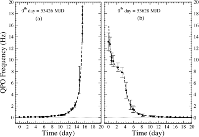
Figure 4.7: (a-c) Variation of QPO frequencies and the shock locations with time (in day) (a) of the rising phase and (b) of the declining phase. The dotted curves are the solutions from oscillating and propagating shocks. While in Fig. (a), the shock appears to be drifting at a constant speed towards the black hole, in Fig. (b), the shock initially moves very slowly and then runs away at a roughly constant acceleration. According to the fitted solution for the rising phase the shock wave goes behind the BH horizon on the $16.14$th day, about $15$ hours after the last observed QPO. In Fig. (c), we showed the shock location variation in both rising and decline phases of the outburst (Chakrabarti et al. 2008a).

In the shock oscillation solution (Molteni, Sponholz & Chakrabarti 1996, Chakrabarti & Manickam 2000, Chakrabarti, Acharyya & Molteni 2004) of QPOs, the oscillations take place at a frequency inverse to the infall time in the post-shock region (i.e., the region between the shock at $r=r_{s}$ and the horizon). In a shock-free low angular momentum flow, this infall time is $t_{infall}\sim r_{s}/v=r_{s}(r_{s}-1)^{1/2}$, where $v=1/(r_{s}-1)^{1/2}$ is the free-fall velocity in a pseudo-Newtonian potential (Paczyński & Wiita, 1980) $\phi_{PN}=-1/(r_{s}-1)$. Here, distance, velocity and time are measured in units of the Schwarzschild radius $r_{g}=2GM/c^{2}$, the velocity of light $c$ and $r_{g}/c$ respectively and where, $G$ and $M$ are the universal constant and the mass of the black hole. However, in the presence of a significant angular momentum capable of producing centrifugal pressure supported shocks around a black hole, the velocity is reduced by a factor of $R$, the compression ratio $R=\rho_{-}/\rho_{+}$, where, $\rho_{-}$ and $\rho_{+}$ are the densities in the pre-shock and the post-shock flows, because of the continuity equation $\rho_{-}v_{-}=\rho_{+}v_{+}$ across a thin shock.

In the presence of a shock, the infall time in the post-shock region is therefore given by

$$t_{infall}\sim r_{s}/v_{+}\sim R~{}r_{s}~{}(r_{s}-1)^{1/2}$$

(Chakrabarti & Manickam 2000, Chakrabarti et al. 2005). Of course, to trigger the oscillation, the accretion rate should be such that the cooling time scale roughly match the infall time scale (Molteni, Sponholz & Chakrabarti 1996). Thus, the instantaneous QPO frequency $\nu_{QPO}$ (in $s^{-1}$) is expected to be,

$$\nu_{QPO}=\nu_{s0}/t_{infall}=\nu_{s0}/[R~{}r_{s}~{}(r_{s}-1)^{1/2}].$$

Here, $\nu_{s0}=c/r_{g}=c^{3}/2GM$ is the inverse of the light crossing time of the black hole of mass $M$ in $s^{-1}$ and $c$ is the velocity of light. In a drifting shock scenario, $r_{s}=r_{s}(t)$ is the time-dependent shock location given by,

$$r_{s}(t)=r_{s0}\pm v_{0}~{}t/r_{g}.$$

Here, $r_{s0}$ is the shock location when $t$ is zero and $v_{0}$ is the shock velocity (in c.g.s. units) in the laboratory frame. The positive sign in the second term is to be used for an outgoing shock in the declining phase and the negative sign is to be used for the in-falling shock in the rising phase. Here, $t$ is measured in seconds from the first detection of the QPO.

The physical reason for the oscillation of shocks appears to be a ‘not-so-sharp’ resonance between the cooling time scale in the post-shock region and the infall time scale (Molteni, Sponholz & Chakrabarti 1996) or the absence of a steady state solution (Ryu, Chakrabarti & Molteni, 1997). In both the cases, the QPO frequency directly gives an estimate of the shock location (Eqn. 4.1). The observed rise of the QPO frequencies with luminosity (e.g., Shaposhnikov & Titarchuk 2006) is explained easily in this model since an enhancement of the accretion rate increases the local density and thus the cooling rate. The resulting drop of the post-shock pressure reduces the shock location and increases the oscillation frequency. In (Chakrabarti & Manickam 2000, Rao et al. 2000) it was shown that QPOs from the higher energy Comptonized photons, thought to be from the post-shock region, (Chakrabarti & Titarchuk, 1995), have a higher $Q$ value. The latter model requires two components, one Keplerian and the other having an angular momentum lower than the Keplerian (referred as sub-Keplerian). This model explains a wide variety of observations of black hole candidates (Smith, Heindl & Swank 2002, Smith, Dawson & Swank 2007). As the shocks are the natural solutions of this sub-Keplerian component, the explanation of QPOs by shocks is natural. When the Rankine-Hugoniot relation is not exactly satisfied at the shock or the viscous transport rate of the angular momentum is different on both sides, the mean shock location would drift slowly due to a difference in pressure on both sides.

Figure 4.7(a-b) shows the variation of the QPO frequencies in the rising (a) and the declining (b) phases of the outburst. The full widths at half maxima of the fitted QPOs have been used as the error bars. In the rising phase (a), the $0^{th}$ day starts on MJD=53426. The fitted curve represents our fit with Eqns. 4.2 & 4.3, which requires that the shock is launched at $r_{s}=1270$ which drifts slowly at $v_{0}=1970$cm s^-1. On the $15^{th}$ day after the outburst starts, the noise was high, but we could clearly observe two different QPO frequencies with a very short time interval. At the time of the last QPO detection ($15.41^{th}$ day) at $\nu=17.78$ Hz, the shock was found to be located at $r\approx 59$. The strength of the shock $R$, which may be strong at the beginning with $R=R_{0}\sim 4$ should become weaker and ideally $R\sim 1$ at the horizon $r=1$, as it is impossible to maintain density gradient on the horizon. If for simplicity we assume the variation of the shock strength as $1/R\rightarrow 1/R_{0}+\alpha t_{d}^{2}$, where $\alpha$ is a very small number limited by the time in which the shock disappears (here $t_{ds}\sim 15.5$days). Thus, the upper limit of $\alpha\sim(1-1/R_{0})/t_{ds}^{2}=0.75/t_{ds}^{2}=0.003$. We find that for a best fit, $\alpha\sim 0.001$ and the reduced $\chi^{2}=0.96$. However, the fit remains generally good ($\chi^{2}=1.71$ for $r_{s0}=1245$ and $v_{0}=1960$cm/s) even with a shock of constant strength ($R=R_{0}$).

In the rising phase of the outburst, it is easy to verify that the QPO frequencies (which are inverses of the infall times from the post-shock flow to the black hole) in the infalling phase are simply related, as though the shock itself is drifting towards the black hole at a slow pace of $\sim 20~{}m/s$ (Chakrabarti et al. 2005, 2008a). A combination of the ram pressure of the incoming flow and rapid cooling in the post-shock region (which lowers the thermal pressure) pushes the oscillating shock inward, shock location decreases and a result of that we observe the increasing nature of QPO frequencies.

During the rising phase of more than two weeks, the disk got sufficient time to transport angular momentum and a dominant Keplerian disk is formed which made the flow soft or very soft. The rapid rise of the black body flux after the QPO disappears and almost total absence of the hard photons testify to the rushing in of the Keplerian disk towards the inner edge (Chakrabarti & Titarchuk, 1995, Ebisawa et al. 1996). If we take the two component advective flow (TCAF) model one step further and actually fit the spectra of a few days spreaded during the outburst we observe, using the same procedure that was followed in Chakrabarti & Mandal (2006b), we can obtain the accretions rates of matter in the Keplerian disk and the sub-Keplerian halo. Table 4.5 gives the rates in units of Eddington rate on various days. It is clear that the Keplerian disk rate steady increases from the beginning while the halo rate changes in a shorter time scale. At the beginning, the halo rate was higher than the disk rate, but in the rest of the time, until the very end the disk rate always dominates. In the soft and the very soft states, the disk rate required to fit the spectra can be high reaching to about two Eddington rates. The hardness/softness diagrams also give an idea of how the accretion rates in the Keplerian and sub-Keplerian components could be changed on a daily basis.

In the declining phase (Fig. 4.7b), the QPO frequency on the first day ($MJD=53631$) corresponds to launching the shock at $\sim r_{s}=40$. It evolves as $\nu_{QPO}\sim t_{d}^{-0.2}$. Since $\nu_{QPO}\sim r_{s}^{-2/3}$ (Eqn. 4.1), the shock was found to drift very slowly with time ($r_{s}\sim t_{d}^{0.13}$) until about $t_{d}=3.5$ day where the shock location was $\sim r=59$. There is a discontinuity in the behavior at this point whose possible origin is obtained from spectral studies presented below. After that, it moves out roughly at a constant acceleration ($r_{s}\sim t_{d}^{2.3}$) and the QPO frequency decreases as $\nu_{QPO}\sim r_{s}^{-2/3}\sim t_{d}^{-3.5}$. Finally, when the QPO was last detected, on $t_{d}=19.92$th day ($MJD=53648$), the shock went as far as $r_{s}=3100$ and the oscillation could not be detected any longer.

6 Dynamic PDS: Observation of the QPO evolution in 3D mode

Figure 4.8: (a-b) Left panel (a) shows the dynamic power density spectra over five days in the rising phase. (1) Obs. ID=91404-01-01-01, QPO=0.382 Hz, (2) Obs. ID=91702-01-01-03, QPO=0.886 Hz, (3) Obs. ID=90704-04-01-00, QPO=2.3130 Hz, (4) Obs. ID=91702-01-02-00, QPO=3.45 & 6.522 Hz with a break frequency at 0.78 Hz and (5) Obs. ID=91702-01-02-01, QPO=14.54 & 17.78 Hz. Right panel (b) shows the dynamic power density spectra over five days in the decline phase. (1) Obs. ID=91702-01-76-00, QPO=13.14 Hz, (2) Obs. ID=91702-01-79-01, QPO=9.77 Hz, (3) Obs. ID=91702-01-80-00, QPO=7.823 & 15.2 Hz with a break frequency at 1.32 Hz, (4) Obs. ID=91702-01-80-01, QPO=4.732 Hz with a break frequency=0.86 Hz, (5) Obs. ID=91702-01-82-00, QPO=0.423 Hz (Chakrabarti et al. 2008a).

For the detailed study of the QPO evolution, we made dynamic PDS. Dynamic PDS is the time dependent power density spectrum, where the variation QPO frequencies (y-axis) and their powers (represented by colours) can be observed with time (x-axis). For making these dynamic PDS, we made $1$ sec time averaged lightcurves and PDS.

Figure 4.8(a-b), presents the dynamic PDS of rising and declining phases of the outburst, where the vertical direction indicates the QPO frequency. The normalized strength of the colours represents the power of the QPOs. It is used to identify the QPO features prominently. These two Figures also show the same day-wise QPO frequency rise and decrease nature, which was observed in Fig. 4.7(a-b).

7 Energy dependent QPO signature

We draw the power density spectra in different energy ranges for the detailed understanding of the origin of QPOs, i.e. to know the exact photon energy ranges are responsible for generating QPOs (Chakrabarti et. al., 2005 & Debnath et. al., 2008a).

Figure 4.9: (a-d) shows PDS of three different energy bands ($2-4$keV, $4-15$keV and $15-60$keV) for different spectral states PCA data. Extreme left panel, (a) shows 3 energy bands PDS of 10th March, 2005 (Obs ID:90704040100) observed data. In the same manner (from 2nd left to right) (b) shows the same energy bands photons’ PDS of March 11th, 2005 (Obs ID:91702-01-02-00G), (c) shows the same energy bands photons’ PDS of May 17th, 2005 (Obs ID:91702015700), and (d) shows the same energy bands photons’ PDS of September 17th, 2005 (Obs ID:91702017900). Here in all the Figures data in both X, Y axes are plotted in logarithmic scales (Debnath et al. 2008a).

In order to quantify the nature of the energy dependence of the power density spectrum, we extracted the lightcurves in three bands with channel numbers 0-8 (2-4 keV), 9-35 (4-15 keV) and 36-138 (15-60 keV) respectively in $0.01$ sec time bins and made their PDS using FTOOLS task ‘powspec’ with normalization factor -2 (to reduce white noise). Figure 4.9(a-d), shows PDS in these three energy bands for $10^{th}$ March, $11^{th}$ March, $17^{th}$ May, and $17^{th}$ September of 2005 data respectively. $10^{th}$ and $11^{th}$ March PDS are of rising hard spectral state, $17^{th}$ May PDS is of intermediate state and $17^{th}$ September PDS is of declining hard spectral state respectively.

We found an interesting nature of the energy dependence on the QPO signatures. In the 10th March data in Fig. 4.9(a), we see the 2.313 HZ QPO in its all three energy bands, whereas just after one day (on 11th March, Fig. 4.9b) the low (2-4 keV) and high (15-60 keV) energy photons do not show any QPO signatures, only intermediate energy (4-15 keV) photons show QPO at frequency 6.522 Hz. On the 10th March, the QPO is originated by the both the pre-shock and post-shock photons; where as on the 11th March only post-shock photons take part on QPO formation.

Intermediate state data of $17^{th}$ May, Fig. 4.9(c) also shows QPO only in the intermediate energy (4-15 keV) band. The observed frequency of the QPO is 18.94 Hz. Here also the post-shock photons of high energy band are responsible for the QPO generation.

Declining hard state data of $17^{th}$ September, Fig. 4.9(d) shows 8.71 HZ QPO in the all three energy bands like Fig. (a), though powers of the QPO at low (2-4 keV) and high (15-60 keV) energy bands are weak and noisy; because in the declining hard state photon count rate decreases due to the less availability of the supply matter from the companion star. Here also like Fig. 4.9(a), both pre-shock and post-shock photons of all energy bands take part in the QPO formation process i.e. oscillates.

8 Compton Cloud oscillations during QPOs in black hole candidates: A comparison with GRS 1915+105

In §4.2.5, we already discussed the origin of QPOs and their evolution under theoretical context. Our POS model is the generalized model for explaining QPO evolutions (Chakrabarti, Nandi, Debnath, Sarkar & Dutta 2005, Chakrabarti, Debnath, Nandi & Pal 2008a and Chakrabarti, Dutta & Pal 2009a) of the transient black hole candidates, those show monotonically rising or decreasing nature of QPO frequencies in their rising or declining outburst phases. We believe that QPOs in the stellar mass black hole candidates originate due to shock oscillations and the frequency is proportional to the inverse of the matter infall time from the location of the shock to the black hole horizon.

In our current work (Debnath, Chakrabarti & Pal, 2010c), we show the nature of the oscillations of the Compton cloud (i.e., CENBOL) during QPOs. The oscillation of the CENBOL not only changes the number of emitted photons causing QPOs (since the intercepted photons change), their other characteristics, such as the temperature and spectral index also change within a single complete oscillation. We demonstrate this by taking the example of QPOs observed in GRO J1655-40 and various classes of GRS 1915+105 and demonstrate that the number of photons intercepted also oscillate. Our procedure is sufficiently general and is applicable to any black hole candidates and also for propagating shocks.

In order to probe what really goes on during a QPO, we consider the lightcurves of GRO J1655-40 and various classes of GRS 1915+105 and picked up regions when the QPO frequency is fairly constant. If $\nu_{QPO}$ is the frequency of QPO, a chunk of data of duration $T_{QPO}=1/\nu_{QPO}$ was taken and was divided into 8 sub-chunks corresponding to eight average phase bins of the oscillations. For each such sub-chunk with time interval $\Delta$T equal to 1/8^th of $T_{QPO}$, we calculate the count rate and the temperature of the black body component of the spectrum. We then plot the variation of the count rate and temperature as a function of the mean phase. This directly shows that the spectral characteristics are also oscillating along with QPOs. This procedure cannot be used for very high frequency QPOs because of low number statistics (i.e., fewer photons in each mean phase of the oscillation) unless the source is unusually bright.

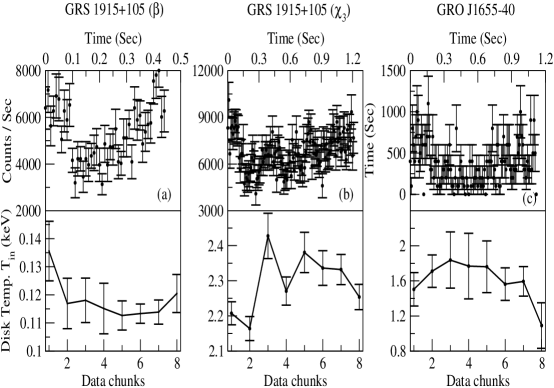
Figure 4.10: (a-c): Variation of the Count rate and disk black body temperature for (a) GRS 1915+105 $\beta$ class, (b) GRS 1915+105 $\chi_{3}$ class and (c) GRO J1655-40 are shown (Debnath et al. 2010c).

Figure 4.10 shows the variation of the photon count rates and disk black body temperature for GRS 1915+105 $\beta$ class, GRS 1915+105 $\chi_{3}$ class and GRO J1655-40 data. For Fig. 4.10(a), we select GRS 1915+105 data of August 31, 1997 (Obs ID:20402-01-44-00), where we found QPO at 2.23 Hz. Each chunk contains data of a time interval ($\Delta$T) of [(1/2.23)*(1/8)] = 0.056 sec. Similarly, Fig. 4.10(b), shows the results of October 14, 1997 GRS 1915+105 data (Obs ID:20402-01-50-00), where we found QPO at 0.849 Hz. Here length of each data chunk is of 0.152 sec. Fig. 4.10(c) is for the GRO J1655-40 data of 9th March, 2005 (Obs ID:91702-01-01-03). Here we observe QPO at 0.886 Hz, so each time chunk duration is 0.14 sec. The QPO fitted results and parameters are summarized in Tab. 4.2. In each of the three plots of the Figure, we observe count rate variation by about $\sim 50\%$. At the same time, we also observe variations in disk black body temperatures and photon indices. These clearly show that sometimes depending on the accretion rate, the count rate may decrease even when the temperature decreases (i.e., the shock recedes away from the black hole).

Table 4.2: QPO fitted results for 3 data sets

Obs.	Obs. Id	UT Date	MJD	$\nu_{QPO}$	$\Delta\nu_{QPO}$	Q	RMS Amp.	$\Delta$T
1	20402-01-44-00	31/08/1997	50691.2557	2.300	0.328	7.01	9.35	0.056
2	20402-01-50-00	24/11/1997	50776.5543	0.849	0.130	6.53	11.6	0.152
3	91702-01-01-03	09/03/2005	53446.0653	0.886	0.132	6.71	15.5	0.140

4.3 Spectral Analysis

For the spectral analysis we mainly used 3 - 25 keV “Standard 2” mode data from RXTE Proportional Counter Unit 2 (PCU2). In general, the black hole energy spectra (2-25 keV) are modeled with ‘diskbb’ and ‘power-law’ components, though sometimes the best fit can be obtained by adding a Gaussian component $\sim 6.5$ keV (for Iron-line).

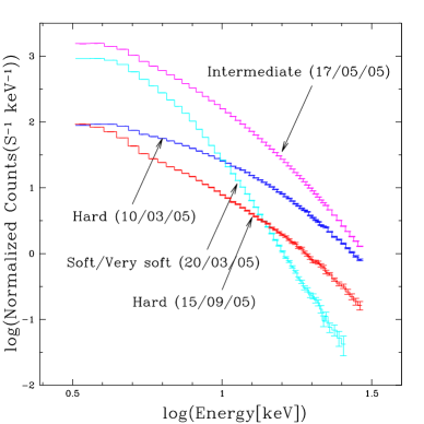
Figure 4.11: RXTE/PCA 3-25 keV spectra of 2005 GRO J1655-40 outburst. Four states are seen.

In our communication (Debnath et al. 2008a) on 2005 GRO J1655-40 outburst, we made a detailed spectral analysis of the $150$ PCA observations of $123$ days in mainly 3 - 25 keV range. Based on the degree of importance of the black body and the power-law components, we divide the entire outburst in four spectral states, namely, hard, soft, very soft and intermediate in the sequence: hard $\rightarrow$ soft/very soft $\rightarrow$ intermediate $\rightarrow$ hard. In our previous communications (Chakrabarti et al. 2005, 2006a, 2008a) we published some significant spectral results as well.

1 Spectral data reduction and fitting

For the spectral study we use PCU2 ‘standard 2’ mode (FS_4a*) data of RTXE/PCA instrument. It is to be noted that for the spectral study background subtraction is very important. For generating background file from the raw data we need to run FTOOLS task ‘runpcabackest’. At first we generate spectral file (*.pha) from raw data and background files independently. Then we need to rebin these pha files using FTOOLS task ‘rbnpha’. Then these rebinned data and background pha files along with response file (*.rsp) can be loaded in FTOOLS XRONOS package (XSPEC) and fitted with physical models.

Black hole energy spectra in low energy X-ray band ($<$ 30 keV), can be fitted with multi-colour disk black body (diskbb) and power-law models. Low energy spectra ($<$ 10 keV) are normally dominated by diskbb component and high energy spectra ($>$ 10 keV) spectra are dominated by power-law component. In our spectral analysis, most of the cases, we used “diskbb + power-law” models. Sometimes for the best-fit, we added an extra component in the form of ‘Gaussian’ (for $Fe$-line) at $\sim 6.5$ keV or ‘CompST’ (for Compton cloud). The best-fit of the data, can be defined as when the value of the fitted reduced $\chi^{2}$ is $\sim 1$. Also we checked the requirement of extra model component for the fitting with the ‘ftest’ task. Table 4.3 summarized ‘ftest’ results for the spectral fittings. We choose the combination of the model components for which the F-test probability is the lowest.

Table 4.3: F-test results for the 4 set of spectra of Fig. 4.12

Obs. Id${{}^{*}*}$	Set 1∗	$\chi^{2}_{red.}$ & d.o.f.∗	Set 2∗	$\chi^{2}_{red.}$ & d.o.f.∗	ftest results†	Remarks
I	diskbb+po	4.009, 50	diskbb+CompST+po	2.582, 47	8.690, 1.078e-04
I	diskbb+po	4.009, 50	diskbb+ga+po	1.019, 48	70.438, 5.266e-15	Set2 used
II	diskbb+po	3.621, 45	diskbb+CompST+po	2.716, 33	0.916, 0.542
II	diskbb+po	3.621, 45	diskbb+ga+po	2.210, 43	10.043, 2.636e-04	Set2 used
III	diskbb+po	2.778, 50	diskbb+CompST+po	0.936, 47	30.811, 3.644e-11
III	diskbb+po	2.778, 50	diskbb+ga+po	0.934, 48	49.804, 1.955e-12	Set2 used
IV	diskbb+po	8.172, 50	diskbb+CompST+po	1.179, 47	92.924, 8.981e-20	Set1 used
IV	diskbb+po	8.172, 50	diskbb+ga+po	4.99, 49	51.358, 3.665e-09

^∗diskbb: disk black body, po: power-law, ga: Gaussian, CompST: Sunyaev-Titarchuk Comptonization model,

 d.o.f.:degrees of freedom.

^∗∗Observation Ids, I: 90704-04-01-00, II: 91702-01-08-00, III: 91702-01-57-00G, IV: 91702-01-79-00

^†F-test was done between Set1 and Set2 model fitted results and F statistic value & probability values are given.

2 Model fitted spectral results

Initial rising hard state spectra (from $25^{th}$ February 2005, MJD = 53426 to $12^{th}$ March 2005, MJD = 53441) were fitted with “diskbb + power-law” and “diskbb + Gaussian + power-law” models. From the spectral fittings, we can conclude that at the very beginning days of this outburst the sub-Keplerian disk component was dominated, but as the day progresses, the Keplerian component became stronger. Another evidence for this is that in the beginning (rising hard state) we found monotonically increasing QPO frequencies in the timing data.

From the spectral fitting we found hard to soft state transition on $13^{th}$ March, 2005 (MJD = 43442). This soft/very soft state (from $13^{th}$ March 2005 to $15^{th}$ May 2005, MJD = 53505) was completely dominated by black body photons (diskbb component). The power-law signature in this state was very little. So, we fitted this state spectra by the standard and simple “diskbb + power-law” model.

Figure 4.12: (a-d) The Figure shows four sets of 3-25 keV PCA fitted spectra. In the top panels we show the model fitted spectra with various components and in the bottom panels we show corresponding reduced $\chi^{2}$ plots. The diskbb, Gaussian and power-law model fitted spectra from the left to the right (a) of 10th March, 2005 (Obs ID:90704040100), (b) of March 20th, 2005 (Obs ID:91702-01-08-00), (c) of May 17th, 2005 (Obs ID:91702015700), and (d) show diskbb, CompST and power-law models fitted spectra of September 17th, 2005 (Obs ID:91702017900) (Debnath et al. 2008a).

We observed the soft to intermediate state transition on $16^{th}$ May, 2005 (MJD = 53506). This intermediate state (from $16^{th}$ May 2005 to $11^{th}$ September 2005, MJD = 53624) was dominated by “diskbb + power-law”, sometimes for the best-fit an extra component Gaussian was added. In this state, we observed QPOs in the timing data, due to local shock oscillations.

From the spectral fitting we observed another state transition from intermediate to hard state on $12^{th}$ September, 2005 (MJD = 53625) during declining state. This hard state (from $12^{th}$ September 2005 to $16^{th}$ October 2005, MJD = 53659) shows interesting spectral features. Initial few days of this state were fitted by “diskbb + CompST + power-law” models. The extra component CompST (Sunyaev-Titarchuk Comptonization model) was needed because of the presence of Compton cloud in the disk, which was different from the cloud generated by the power-law. After this the spectra were fitted with normal “diskbb + power-law” or “diskbb + gaussian + power-law” models.

Table 4.4: Spectral fit results for the 4 sets of spectra of Fig. 4.12

Obs. Id	UT Date	Photon	Flux (in $10^{-9}ergs~{}cm^{-2}~{}s^{-1}$)		$\chi^{2}_{red}$
		Index($\Gamma$)	3-10keV	10-25keV
90704-04-01-00	2005-03-10	1.766	1.849	1.533	1.019
91702-01-08-00	2005-03-20	6.164	2.416	0.804	2.210
91702-01-57-00G	2005-05-17	2.711	46.86	11.75	0.934
91702-01-79-00G	2005-09-17	1.691	1.838	1.065	1.179

Figure 4.12 shows 4 sets of spectral plots with model components and their corresponding $\chi^{2}_{red}$ plots. These four sets of the spectra were taken from 4 different spectral states’ observational data. A summary of the spectral fitted parameters of the four sets of spectra are presented in Tab. 4.4.

We also fitted the spectra of a few days with TCAF model (using the same procedure as in Chakrabarti & Mandal, 2006b) and from our fittings we obtained accretion matter flow rates for the two components of accretion flows (the Keplerian or disk rate and the sub-Keplerian or halo rate). These results are summarized in the following Tab. 4.5.

Table 4.5: Theoretically fitted GRO J1655-40 outburst data with TCAF model

Date	MJD	Halo rate	Disk rate
Mar. 3, 2005	53432.7930	0.015	0.0100
Mar. 9, 2005	53438.0539	0.004	0.0400
Mar. 10, 2005	53439.7400	0.009	0.0650
Mar. 11, 2005	53440.6780	0.0043	0.5100
Mar. 12, 2005	53441.5109	0.0100	0.7800
May 16, 2005	53506.9531	0.0550	1.5640
May 20, 2005	53510.0994	0.0560	1.7400
Sep. 16, 2005	53629.3761	0.0038	0.0700
Sep. 19, 2005	53632.4557	0.0029	0.0300
Sep. 22, 2005	53635.4696	0.0065	0.0140
Sep. 29, 2005	53641.0383	0.009	0.0100

3 Daily variation of fluxes and spectral parameters

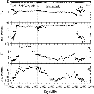
Figure 4.13: (A-B): Left panel (A) shows the fitted parameters of RXTE 3 - 25 keV PCA spectra are plotted with time (MJD). The panels are: (a) disk black body temperature (T_in) in keV, (b) disk black body normalization, (c) power-law photon index ($\Gamma$) and (d) power-law normalization plotted with day. Logarithmic scale is used in the y-axis and the error bars are at $1\sigma$ level. Right panel (B) shows the daily flux variations. The panels are: (a) 3 - 25 keV total flux, (b) 3-10 keV bolometric disk black body flux, (c) 10-25 keV power-law flux and (d) the ratio of the total and power-law fluxes. In the soft/very soft and intermediate states the total flux is dominated by the black body flux. Only in the hard states of the rising and declining phases the ratio is less than unity. Here we also use logarithmic scales along the y-axis (Debnath et al. 2008a).

To get a clear idea about the spectral evolution in the GRO J1655-40 outburst of 2005, we fitted PCU2 data of RXTE/PCA instrument in 3 - 25 keV energy range for the total of $150$ observations of $123$ days data. From the spectral fits we found disk black body temperature ($T_{in}$) in keV, normalization factors for black body, power-law photon index ($\Gamma$) and its normalization factor components. Also we found Gaussian and CompST fitted parameters, where they were needed for the fitting. We also calculated disk black body (mainly in 3-10 keV energy range), power-law (mainly in 10-25 keV energy range) and total (in 3-25 keV energy range) fluxes.

From the nature of the variation of the power-law indices and the disk black body components of Fig. 4.13(A), we classified the full outburst into four spectral states: (i) Hard state from from 25^th of February, 2005 (MJD = 53426) to 12^th of March, 2005 (MJD = 53441), (ii) Soft/Very soft state from 13^th of March, 2005 (MJD = 53442) to 15^th of May, 2005 (MJD = 53505). (iii) Intermediate state is from 16^th of May, 2005 (MJD = 53506) to 11^th of September, 2005 (MJD = 53624) and finally (iv) Hard state from the 12^th of September, 2005 (MJD = 53625) till 16^th of October, 2005 (MJD = 53659). We kept the hydrogen column density (N_H) fixed at 7.5$\times$ 10²¹ atoms cm^-2 and the systematics at $0.01$.

Daily variations of the fitted parameters are plotted in Fig. 4.13(A), which clearly reveals the justification of separating the full outburst in the above mentioned four states. The panels (a-d) are respectively the black body temperature $T_{in}$ in keV, the black body normalization factor, the photon index $\Gamma$ and the power-law normalization (plotted in the log scale along Y-axis).

Figure 4.14: The spectral evolution for the hard state in the rising phase from 25^th of February, 2005 to 12^th of March, 2005. Though the spectral slope remains more or less constant for the first twelve days or so, the intensity of radiation increase steadily. Subsequently, the spectral slope (i.e., photon index $\Gamma$) and total flux both increase monotonically (Chakrabarti et al. 2006a).

Daily variations of the total flux (panel a), black body flux (panel b) and the power-law flux (panel c) are shown in Fig. 4.13(B). The panel (d) shows how the ratio of the black body to total flux changes daily. Generally in the soft and very soft states the ratio is almost unity, indicating the dominance of the soft component in both of these divisions. However, in Fig. 4.13(A), we observe a distinct difference in power-law normalization and power-law index in these two states. The QPOs are observed only in certain days of the intermediate state. It may be noted that $\Gamma$ obtained right in the middle of the soft/very soft state is unphysically high ($>4$). We believe that this is due very poor statistics (e.g., only one good PCU of RXTE, PCU2 was working properly and photon energy was $>20$keV) rather than any unusual absorption at high energies. We find that other workers (Saito et al. 2006) also reported a high photon index for these observations.

In Fig. 4.14, the spectral variations for the initial hard state are shown. From the Figure it is observed that though in the initial few days spectral slopes and fluxes were remained more or less constant, but these parameters were increased monotonically in the subsequent days. This is another indication that the Compton cloud moved inward during the rising phase of the outburst.

Chapter 4 GX 339-4: A Transient Low-mass X-ray Binary

GX 339-4 is a well known stellar-mass Galactic black hole candidate. This bright variable X-ray source was first observed by MIT X-ray detector aboard OSO-7 Satellite (Markert et al. 1973) in the energy range of 1-60 keV. GX 339-4, a transient Low Mass X-ray Binary (LMXB) system is located at $(l,b)=(338^{\circ}.93\pm 0.20,-4^{\circ}.27\pm 0.20)$ (Markert et al. 1973) with R.A.=$16^{h}58.8^{m}\pm 0.8^{m}$ and Dec.= $-48^{\circ}48^{\prime}\pm 12^{\prime}$. Optical spectroscopic study indicates mass function of the source is $M$ = $5.8\pm 0.5~{}M_{\odot}$ and distance $D$ = $6$ kpc (Hynes et al. 2003, 2004).

5.1 The recent outburst

Since its discovery, GX 339-4 has undergone several outburst phases during which the source was observed in energy bands from radio to high energy X-ray to reveal its multi wavelength nature (Makshima et al. 1986, Liu et al. 2001, Homan et al. 2005). During the RXTE era, this source exhibits frequent X-ray outbursts (1998, 2002/2003, 2004/2005, 2006/2007) at 2-3 years of interval with very low luminosity states in between each episode. The complex outburst profile in each epoch generally begins and ends in the low/hard state, which is quiet common in other outbursting black hole candidates (e.g., GRO J1655-40, XTE J1550-564). This general behaviour is understood to be due to sudden variation of viscosity in the system (Mandal & Chakrabarti 2010) which causes the Keplerian disk to rush in. The temporal and spectral state evolution during the previous outbursts are well studied (Nowak et al. 1999, Belloni et al. 2005, Motta, Belloni & Homan 2009) but still not clearly understood due to the complex nature of the accretion process in the system. Miller et al. (2004) has reported this black hole candidate to be a rotating Kerr-black hole with a low spin value of around zero.

Recently, after 3 years of remaining in the quiescent state, the source GX 339-4 became again X-ray active on January 03, 2010 with the first detection by MAXI/GSC onboard ISI (Yamaoka et al. 2010). Immediately after the announcement of X-ray trigger, RXTE has started monitoring the transient source from Jan 12, 2010 (Tomsick, 2010). Other scientific space satellites (Swift, INTEGRAL, etc.) are also observing this source in regular intervals. We studied timing and spectral properties of the source in its initial outburst phase, using RXTE archival data (Debnath et al. 2010a). Now we present these results obtained from the current rising phase of the GX 339-4 outburst using RXTE data of PCA and ASM instruments for an analysis of a total of $30$ observational data which are spreaded over the period of $5{th}$ March, 2010 (MJD = 55260) to $29{th}$ April, 2010 (MJD = 55315). From our detailed timing and spectral analysis of the initial phase of the outburst, we classified the initial rising phase of the GX 339-4 outburst mainly in three spectral states, hard, hard/intermediate and soft/intermediate. Spectra up to $9^{th}$ of April 2010 were at ’pure’ hard state. After that up to $17^{th}$ of April it is in hard/intermediate state and then finally after April $18$ it moved to soft/intermediate state. During this outburst phase, on $10^{th}$ of April 2010, we observe a state transition between hard-hard/intermediate states and on $18^{th}$ of April 2010 another state transition between hard/intermediate-soft/intermediate spectral states. The results are given in Debnath et al. (2010a).

5.2 Results of the timing analysis

For studying timing properties of the recent GX 339-4 outburst, we use archival data of RXTE PCA and ASM instruments. For the PCA data analysis, we mainly use most stable and well conditioned proportional counter unit 2 (PCU2) data. NASA’s standard analysis software package (Heasoft 6.8) is used for the detailed timing as well as spectral analysis of the current GX 339-4 outburst. In the study of the temporal properties of any black hole candidate, finding quasi-periodic oscillations (QPOs) in power density spectra (PDS) is as important as observation of the photon count/flux variations. Generally, most of the black hole candidates (BHCs) show low frequency QPOs in the frequency range between $0.01$ to $30$ Hz (Remillard et al. 1999, Debnath et al. 2008a). Some BHCs (GRO J1655-40, GRS 1915+105, XTE J1859+226, H1743-322 etc.) also show the signatures of dual high frequency QPOs in 3:2 ratio (Remillard et al. 1999, Cui et al. 2000, Strohmayer 2001, Belloni et al. 2006, Remillard et al. 2006).

We studied temporal properties of the initial phase of the GX 339-4 outburst in a systematic manner. First we extracted lightcurves from the ‘Event mode’ data using FTOOLs task ‘sefilter’ in both $1$ sec and $0.01$ sec time bins. Later $0.01$ sec time bin lightcurves are used to make PDS using FTOOLs task ‘powspec’, which actually do FFTs of the lightcurves. From the PDS we tried to find QPO signatures and further it was fitted with the model ‘Lorentzian’ line profile to find centroid QPO frequency, FWHM and its highest power.

During initial outburst phase, initially the source was in the hard state without any signature of QPO in the PDS up-to 3rd week of March, 2010. We first observed $102$ mHz QPO on March $22$, 2010. After that the QPO frequency monotonically increased up to $5.69$ Hz (observed on April $17$, 2010) within $\sim 26$ days. Afterwards, QPOs were on and off sporadically (e.g., $5.739$ Hz on April $18$, 2010, $5.677$ Hz on April $22$, 2010 and $5.913$ Hz on April $29$, 2010), always remaining roughly at the same value. In the soft/intermediate state, we have not seen any signature of QPOs from April $19$th - $21$st, 2010 and from April $23$th - $28$th, 2010. In the PDS, we also interestingly found $3$ harmonics of primary node $2.42$ Hz QPO on April $13$, 2010 (Yu, 2010), generally $2$ harmonics of a QPO frequency are seen.

The monotonically rising nature of the QPO frequencies (from $22$nd of March 2010 to $17$th of April 2010) in the initial outburst phase was fitted with theoretical model of the propagating oscillatory shock (POS). We followed the same procedure, what we had used to fit the QPO evolution of GRO J1655-40 initial rising phase of 2005 outburst (Chapter 4), where we also observed monotonically increasing nature of QPO frequencies. From the model fitting, we calculated initial shock location at $1500~{}r_{g}$ (on $5{th}$ March, 2010, where we first observed QPO at $0.102$ Hz), where $r_{g}=2GM/c^{2}$, Schwarzschild radius and final shock location at $172~{}r_{g}$ on $17{th}$ April, 2010 and initial and final compression ratios, $R$ ($4$ & $0.99$), which are inverse of the shock strengths, $\beta$ ($=1/R$). The compression ratio (R) is ratio between the pre-shock and the post-shock densities, i.e., $R=\rho_{-}/\rho_{+}$, where, $\rho_{-}$ and $\rho_{+}$ are the densities in the pre-shock and the post-shock flows. We also found shock wave moves towards the black hole in at a roughly constant speed of $\sim 10~{}m~{}s^{-1}$.

Figure 5.1: Left panel (Fig. A) shows the RXTE ASM lightcurve and hardness ratio plots for the black hole candidate GX 339-4 during the RXTE era (1996 to April, 2010) and right panel (Fig. B) shows the same thing in recent 2010 GX 339-4 outburst. In each Figure, the top panel (a) is the 2-12 keV ASM lightcurve and (b) is the hardness ratio (5-12 keV vs. 2-5 keV count ratio) as a function of the MJD of the event are plotted. The vertical dashed line at MJD $55296$ in (B), indicates the day of state transition from hard to hard/intermediate spectral states. The other vertical dashed line at MJD $55304$ indicates the state transition from hard/intermediate to soft/intermediate (Fig.B: Debnath et al. 2010a).

Since on the $18^{th}$, $22^{nd}$ and $29^{th}$ of April, $2010$, we observed QPOs in $\sim 5.7$ Hz, nearly same QPO frequency as was observed on the $17^{th}$ April, last day of our theoretical model fit, we can conclude that the shock wave became steady and oscillated nearly at the same locations in the soft/intermediate state. According to our model in these three observation days, we found that the value of the compression ratio (R) to become less than unity, which is unphysical for a stable propagating shock. As $R$ became less than unity at $\sim 175r_{g}$, quite before the black hole horizon, we can conclude that the shock was not able to fall into the black hole. This was also observed during the initial rising phase of 2005 GRO J1655-40 outburst (Chakrabarti et al. 2008a, Debnath et al. 2008a).

1 ASM Light Curve

RXTE ASM data (Levine et al. 1998) were downloaded and analyzed in different energy bands (2-3, 3-5, 5-12 & 2-12 keV). In Fig. 5.1, 2-12 keV ASM lightcurves (counts/sec) and the ASM hardness ratios (ratio between the photon count rates in 5-12 keV and 2-5 keV bands) are plotted for the RXTE ASM data (Fig. 5.1A) from 6th January, 1996 (MJD = 50088) to 6th May, 2010 (MJD = 55322) for the BHC GX 339-4 and for its ASM data of the current 2010 outburst (Fig. 5.1B) (from 12th January 2010 (MJD = 55208) to 6th of May 2010). In the RXTE era so far the transient BHC GX 339-4 has shown five outbursts including the present one.

2 Hardness-Intensity Diagram

We extracted and analyzed the PCA (Jahoda et al., 1996) data of the initial rising phase of the outburst from point $A$, $5^{th}$ of March 2010 (MJD = 55260) to April 29, 2010 (MJD = 55315). Figure 5.2 shows RXTE PCA hardness-intensity diagram (HID) (Mandal & Chakrabarti 2010). In Fig. 5.2, the PCA 3-20 keV count rate of the above mentioned period against the X-ray color (PCA count ratio between 6-20 keV and 3-6 keV energy bands) are plotted. It is evident from the Figure that initially the source was at ’pure’ hard state up to $9^{th}$ of April 2010. Subsequently, it went to the hard/intermediate state for a short duration of period from April $10$, 2010 (point B) to April $17$, 2010. Finally from $18^{th}$ of April 2010 (point $C$) it went to the soft/intermediate state. We observed low-frequency QPOs in all the three spectral states, which are most common phenomena for low-mass X-ray black hole binaries.

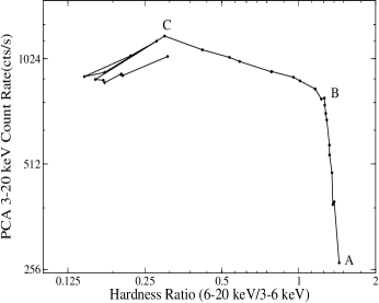
Figure 5.2: The Hardness Intensity Diagram (HID) observed with RXTE PCA. The y-axis of the plot represents the PCA count rates in 3-20 keV energy band and the x-axis represents the hardness ratio between the count rates of the energy bands of 6-20 keV and 3-6 keV bands. Both axes are in logarithmic scales. Point $A$ means MJD 55260, start date of our observation, $B$ means MJD 55296 and $C$ means MJD 55304. Source was in a ’pure’ hard state between the days of point A & B, was at a hard/intermediate state between the days of point B & C and finally after point C, it moved to the soft/intermediate state (Debnath et al. 2010a).

3 Light curves and Hardness, Softness diagrams

For the detailed study of the X-ray photon count variations over the initial rising phase of the outburst, we extracted 2-15 keV (0-35 Channels) PCA lightcurves with time bin of 1 sec. Also, we studied both the hardness and softness ratio variations. These lightcurves were extracted using FTOOLS taskes “sefilter” & “seextrct” on Event mode data. To plot the lightcurves “fplot” task was used. The hardness and the softness ratio diagrams were made by extracting lightcurves for three energy bands: $A:0-8$ channels ($2-4$ keV), $B:9-35$ channels ($4-15$ keV) and $C:36-138$ channels ($15-60$ keV). A hardness diagram is the plot between $C/A$ (HR2) vs. $B/A$ (HR1), while the softness diagram is the plot between $B/C$ (HR3) vs. $A/C$ (HR4).

Figure 5.3: (a-d):In the lower panel, 2-15 keV (0-35 Channels) PCA lightcurve and in the upper panel the hardness and softness diagrams are plotted. In hardness diagrams, the dashed horizontal ($B=A$), vertical ($C=A$) and the dotted line ($B=C$) are for reference purpose. In softness diagram they represent $C=A$, $B=C$ and $A=B$ respectively. Observation dates are: (left to right) (a) on 5th of April, 2010 (Obs ID:95409-01-13-02), (b) on 13th April, 2010 (Obs ID:95409-01-14-06), (c) on 16th of April, 2010 (Obs ID:95409-01-15-00), and (d) on 28th of April, 2010 (Obs ID:95409-01-16-04). Fig. (a) is taken from the ’pure’ hard state, where as Figs. (b) & (c) are taken from the hard/intermediate state and remaining Fig. (d) is taken from soft/intermediate states. In Fig. (d) x, y scale for the hardness and softness diagrams are changed.

Our motivation of splitting the lightcurves in above mentioned energy bands is to separate the low energy Keplerian disk photons ($\lower 2.15277pt\hbox{$\;\buildrel<\over{\sim}\;$}4$ Kev) from the high energy sub-Keplerian disk photons. Thus, $A$ would be emitted mostly from the Keplerian component. The component $B$ would be emitted from the region where the moderate thermal Comptonization of the Keplerian photons took place. The component $C$ would be emitted from the region which was definitely depleted or enhanced during state transitions as it was represented at the higher energy side of the pivotal energy [$\sim 15$ keV] in the spectrum. Thus, these diagrams are not directly connected to the spectral states – rather, they are connected to the geometry, i.e., the number of soft photons produced by the Keplerian disk ($\sim A$) and the seed photons intercepted by the ‘Compton cloud’ [$\sim(B+C)$] and the number of scatterings they undergo ($\sim B$ or $\sim C$).

From the Fig. 5.3(a-d), we got a rough idea about the evolution of accretion rates of high energy, the sub-Keplerian (halo) and low energy, the Keplerian (disk) seed photons during the initial rising phase of the outburst.

4 Power Density Spectra

Power Density Spectra (PDS) were generated by using “powspec” task of XRONOS package with a normalization factor of ‘$-2$’ to reduce ‘white’ noise from the rms fractional variability. We also used a geometrical factor of $-1.02$ to get a nearly equispaced logarithmic frequency bins. The power has been obtained in units of $rms^{2}/Hz$. The lightcurve of X-ray variability from which PDS was obtained were binned at $0.01$ sec time resolution so that the Nyquist frequency (for higher limit) becomes $50$ Hz. It general practice for studying PDS, is to find QPO. QPOs are generally Lorentzian type (Nowak 2000, van der Klis 2005) and thus we fitted each PDS by zooming QPO peak with Lorentzian profile to find the centroid frequency and width of each observed QPO. Table 5.1 shows the observed QPO frequencies and their fitted parameters.

Figure 5.4: (a-d): (a) The model fitted PDS of $5^{th}$ April, 2010 (Obs. ID:95409-01-13-02), example of a typical hard state. QPO was found at $0.317$ Hz. (b) The model fitted PDS of $13^{th}$ April, 2010 (Obs. ID:95409-01-14-06). Here we observed 3 harmonics of the primary $2.42$ Hz QPO (other two harmonics are $4.84$ Hz and $7.19$ Hz). (c) The model fitted PDS of $16^{th}$ April, 2010 (Obs. ID:95409-01-15-00), a typical day just 1 day before hard-soft/intermediate state transition. The QPOs were observed at frequencies $4.177$ and $8.192$ Hz. (d) The model fitted PDS of $29^{th}$ April, 2010 (Obs. ID:95409-01-16-05), a typical day of soft/intermediate state. Here we observed strong signature of intermediate state QPO at $5.913$ Hz frequency.

In Tab. 5.1, we present a summary of the QPO fitted results, where we put the centroid frequency ($\nu$) of the QPO, its width ($\Delta\nu$) (both in Hz), the coherence parameter or Quality factor $Q$ (= $\nu$/$\Delta\nu$) and percentage of RMS amplitude. The RMS amplitude ($R$) of the fitted QPO was calculated from the relation $R=100~{}\sqrt{(I/mean~{}count~{}rate)}$, where, $I$ is the integral of the Lorentzian profile of the fitted QPO. Our selection criterion for defining a peak at PDS as QPO was the value $Q$ parameter, for QPO it should have to be more than 2 ($Q>2$).

Figure 5.4(a-d) shows the QPO fitted PDS of the initial rising phase of the outburst, taken from different spectral states. First Figure is taken from the ’pure’ hard state data, next two are taken from the hard/intermediate state data and the remaining last Figure is taken from the soft/intermediate state data. In the intermediate state, sometimes we observe QPOs in PDS and sometimes we do not. This may be because the generation of the shock due to collision of incoming Keplerian matter and receding sub-Keplerian matter.

Figure 5.5: The variation of the PDS with QPO frequencies of the initial rising phase of the outburst. The dates (dd/mm), the observation ID and the frequency of the QPOs are in the inset. Arrows indicate the direction in which the dates are increasing.

Figure 5.5 shows the date-wise QPO evolution of the initial rising phase of the most recent GX 339-4 outburst. $16$ PDS plots are drawn. In the insets of each PDS observation ID, observation date and QPO frequency/frequencies if observed are noted. Arrows indicate the direction in which the dates are increasing. Our first plot is of $19^{th}$ March, 2010 data, three days before first observed QPO and second plot is of $22^{nd}$ March, 2010 data, where we observed QPO at $102$ mHz (our first observed QPO). We fitted the QPO evolution up to $17^{th}$ April, 2010 data (where we observed QPO at $5.692$ Hz). After that we also found QPOs at frequencies $5.739$ Hz on April 18, 2010, $5.677$ Hz on April 22, 2010 and $5.913$ Hz on April 29, 2010 (not shown in Figure). These last three observed QPOs are of soft/intermediate state.

Table 5.1: Observed QPO fitted parameters for recent GX 339-4 outburst

Obs. ID	UT Date	$\nu$	$\Delta\nu$	Q	RMS Amp.
95409-01-11-02	2010-03-22	0.102	0.0318	3.207	17.438
95409-01-11-03	2010-03-24	0.113	0.0452	2.500	18.879
95409-01-12-00	2010-03-26	0.133	0.0443	3.002	18.276
95409-01-12-03	2010-04-01	0.202	0.0624	3.237	19.044
95409-01-13-00	2010-04-03	0.261	0.0802	3.254	17.158
95409-01-13-02	2010-04-05	0.317	0.0845	3.751	16.952
95409-01-13-05	2010-04-06	0.363	0.0377	9.628	15.391
95409-01-14-00	2010-04-09	0.547	0.1088	5.027	16.346
95409-01-14-01	2010-04-10	1.026	0.1261	8.136	14.074
95409-01-14-02	2010-04-11	1.241	0.2192	5.661	9.278
95409-01-14-02	2010-04-11	2.488	0.3328	7.475	12.098
95409-01-14-03	2010-04-12	1.588	0.2509	6.329	9.095
95409-01-14-03	2010-04-12	3.156	0.3433	9.193	9.575
95409-01-14-06	2010-04-13	2.420	0.1502	16.11	8.412
95409-01-14-06	2010-04-13	4.842	0.4634	10.45	5.824
95409-01-14-06	2010-04-13	7.193	1.4608	4.924	5.847
95409-01-14-04	2010-04-14	2.374	0.1787	13.28	9.175
95409-01-14-04	2010-04-14	4.727	0.7466	6.331	6.434
95409-01-14-05	2010-04-15	3.643	0.2659	13.70	9.137
95409-01-14-05	2010-04-15	7.308	1.1724	6.233	5.962
95409-01-15-00	2010-04-16	4.177	0.6248	6.685	8.738
95409-01-15-00	2010-04-16	8.192	1.3115	6.246	5.390
95409-01-15-01	2010-04-17	5.692	0.9941	5.725	7.297
95409-01-15-01	2010-04-17	11.42	2.9427	3.880	4.950
95409-01-15-02	2010-04-18	5.739	0.5257	10.92	6.794
95409-01-15-05	2010-04-21	- - - -	- - - -	- - - -	- - - -
95409-01-15-06	2010-04-22	5.677	0.4053	14.01	6.150
95409-01-15-06	2010-04-22	11.09	1.4958	7.414	1.814
95409-01-16-04	2010-04-28	- - - -	- - - -	- - - -	- - - -
95409-01-16-05	2010-04-29	5.913	1.0369	5.703	6.741

5 QPO evolution in the rising phase of the outburst and POS Model

We fitted monotonically day-wise increasing nature of the QPO frequencies with our propagating oscillatory shock (POS) model. We followed the same methodology as was followed for fitting of the QPO evolution of the initial rising phase of 2005 GRO J1655-40 outburst. For the present QPO evolution, we take observed QPOs from $22^{nd}$ of March, 2010 to $17^{th}$ of April, 2010. In this period, we saw that QPO frequencies were increased monotonically from $102$ mHz to $5.69$ Hz with in a period of $\sim 26$ days. Spectral analysis (discussed in the next Section) indicates during the above mentioned evolution period photon indices of the spectra were less than $2$, i.e., source was at ’pure’ hard state (up to $9^{th}$ of April) and hard/intermediate state ($10^{th}$ April to $17^{th}$ April). After that on the $18^{th}$ of April 2010, photon index became $\sim 2.5$, the source was moved to the soft/intermediate spectral state. From the analysis, we found hard to hard/intermediate transition on $10^{th}$ of April 2010 and hard/intermediate to soft/intermediate spectral state transition on $18^{th}$ of April 2010. In this soft/intermediate state, we also observed QPOs at frequencies $5.739$ Hz, $5.677$ Hz & $5.913$ Hz respectively on 18th, 22nd & 29th of April 2010.

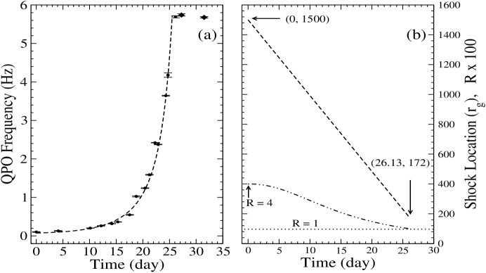
Figure 5.6: (a-b): (a) Variation of QPO frequency with time (in day) of the initial rising phase of the outburst with fitted POS model (dotted curve). The diamonds indicate the last two observed QPOs (on April 18 & 22, 2010) in the soft/intermediate spectral state, not included in our model fitting, since the shock already achieved its weakest strength with compression ratio (inverse of shock strength $\beta$) $R\sim 1$, on earlier day, April $17^{th}$. (b) Variation of the shock location (in $r_{g}$) and compression ratio ($R$) multiplied by $100$ are plotted (Debnath et al. 2010a).

The governing equations for our theoretical POS model fitting for the present GX 339-4 QPO evolution are the same as mentioned in the previous Chapter (Eqns. 4.1-4.3) for GRO J1655-40 evolution, except that here the shock strength ($\beta=1/R$) is assumed to vary by the relation $1/R\rightarrow 1/R_{0}+\alpha t_{d}^{2.15}$, where $R_{0}$ is the initial compression ratio, $t_{d}$ is the time in day (taking first observed QPO frequency day as $0^{th}$ day) and $\alpha$ is a very small number ($6.8\times 10^{-4}$), limited by the time in which the shock disappears. We started with strong shock ($R_{0}=4$), which becomes unity in $\sim 26$ days on $17^{th}$ of April, 2010. Physically, shock strength $\beta=1$, i.e., $R=1$ means, the system is in equilibrium condition with matter densities of pre- and post-shock are same; no propagating shock oscillation is possible. Although after $17^{th}$ of April, we found QPOs near around $5.7$ Hz in the soft/intermediate state, this is because of local oscillation near about same location due to the generation of the shock wave by the incoming Keplerian matter and receding sub-Keplerian matter. This type of behaviour is also observed in 2005 GRO J1655-40 outburst, where we found QPOs in the intermediate state at frequencies around $19$, $17$ and $13$ Hz.

From the fitting, we calculated initial shock location at $1500~{}r_{g}$ (on $5{th}$ March, 2010, where we first observe QPO at $0.102$ Hz), where $r_{g}=2GM/c^{2}$, Schwarzschild radius and final shock location at $172~{}r_{g}$ on $17{th}$ April, 2010 and initial and final compression ratios ($4$ & $0.99$). Since in this current rising phase of GX 339-4 outburst, shock strength ($\beta$) reaches its weakest value unity at $\sim 175~{}r_{g}$, much before the black hole horizon, we can conclude that the shock was not able to fall into the black hole. This was also observed in the rising phase of 2005 GRO J1655-40 outburst (Chakrabarti et al. 2008a). From our theoretical POS model fitting, we also found that the shock wave was moved towards the black hole with a constant velocity ($\sim 10~{}m~{}s^{-1}$).

6 Energy dependent QPO signature

In order to quantify the energy dependent nature of the power density spectra, we extracted the lightcurves using PCU2 data of RXTE PCA instrument in three different energy bands with channel numbers 0-8 (2-4 keV), 9-35 (4-15 keV) and 36-71 (15-30 keV) respectively in $0.01$ sec time bins and made their PDS using FTOOLS task ‘powspec’ with normalization factor -2 (to reduce white noise) and geometric area factor -1.02 (to get a nearly equispaced logarithmic frequency bins). Our motivation of splitting the 2-30 keV PDS in above mentioned energy bands is to separate the low energy Keplerian disk photons ($\lower 2.15277pt\hbox{$\;\buildrel<\over{\sim}\;$}4$ Kev) from the high energy sub-Keplerian disk photons. Thus, 2-4 keV PDS would be mostly dominated by the Keplerian component, 4-15 keV PDS would be emitted from the region where the moderate thermal Comptonization of the Keplerian photons took place and higher energy band (15-30 keV) PDS would be dominated by the non-thermal sub-Keplerian component.

Figure 5.7: (a-c): PDS of three different energy bands of three different observation IDs, taken from initial, middle and final stages of the initial rising phase outburst. In each Fig. top panel is for 2-4 keV, middle panel is for 4-15 keV and bottom panel is for 15-30 keV bands. (Left) Fig. (a) is for Obs ID:95409-01-13-02 (observed on 5th April, 2010), (middle) Fig. (b) is for Obs ID:95409-01-14-06 (observed on 13th April, 2010) and (right) Fig. (c) is for Obs ID:95409-01-15-00 (observed on 16th April, 2010). Fig. (a) is for initial QPO evolution phase, where all the three energy bands show QPO signature, whereas (c) is for final QPO evolution phase, only the intermediate energy photons take part into QPO formation. Fig. (b) is a special PDS, where we found 3 QPO harmonics (Yu 2010) of $2.42$ Hz primary node frequency QPO. Here, the higher energy band photons do not show other two harmonics (Debnath et al. 2010a).

Figure 5.7(a-c) shows energy dependent PDS of the three different observation IDs data, taken from very beginning, middle and final stages of GX 339-4 initial rising phase of the QPO evolution process. Figure 5.7(a) represents the energy dependent PDS of 95409-01-13-02 observation data (observed on $5^{th}$ of April 2010). Here, the X-ray photons of all the three energy bands take part into the generation of $0.317$ Hz QPO. Similarly, in Figure 5.7(c), the energy dependent PDS of April $16^{th}$, 2010 (observation ID: 95409-01-15-00) are plotted. Here only intermediate energy photons take part into the generation process of $4.177$ Hz QPO. In Figure 5.7(b), the energy dependent PDS of observation ID: 95409-01-14-06 (observed on $13^{th}$ of April 2010) is shown. In this particular observation we found two more harmonics of fundamental $2.42$ Hz. From the Figure, we observe X-ray photons of all the three energy bands taking part into the generation of $2.42$ Hz QPO, but higher energy photons do not take part into the generation of other two harmonics ($4.84$ & $7.19$ Hz QPO).

5.3 Results of spectral analysis

For the spectral study we use $3-30$ keV PCU2 ‘standard 2’ mode (FS_4a*) data of RTXE/PCA instrument. It is to be noted that for the spectral study the background subtraction is very important. For generating background file from the raw data we ran FTOOLS task ‘runpcabackest’. At first we generate spectral pulse height analysis (pha) files from the both raw data and the background files independently. Then we rebinned these pha files using FTOOLS task ‘rbnpha’ and finally these rebinned source and and background pha files along with response file (*.rsp) were loaded in FTOOLS XRONOS package (XSPEC) and fitted with physical models.

Black hole energy spectra in low energy X-ray band ($<$ 30 keV), can be fitted with multi-colour disk black body (diskbb) and power-law models. Low energy spectra ($<$ 10 keV) are normally dominate by thermal diskbb component and high energy spectra ($>$ 10 keV) are dominated by non-thermal power-law component.

In the current rising phase of the outburst, we made detailed spectral analysis of a total of $30$ observational IDs data which are spreaded over the period of $5{th}$ March, 2010 (MJD = 55260) to $29{th}$ April, 2010 (MJD = 55315). For the spectral data analysis, XSPEC package of version 12.5 were used, and for all observations we kept the hydrogen column density ($N_{H}$) fixed at $5\times 10^{21}$ (Motta et al. 2009) using absorption model wabs. We fitted the spectra of each day, using standard diskbb and power-law models with a Gaussian line (for Fe emission line at $6.5$ keV).

Figure 5.8: Variation of RXTE PCA count rates in (a) 15-30 keV, (b) 4-15 keV and (c) 2-4 keV energy bands are plotted in top three panels and in the bottom panel power-law photon index variation with day (in MJD) are plotted. The vertical dashed line at MJDs $55296$ and $55304$ indicates the state transitions between hard to hard/intermediate to soft/intermediate states (Debnath et al. 2010a).

From the detailed spectral analysis we can conclude that the source was initially in the ’pure’ hard state up to $9^{th}$ of April, 2010 (MJD = 55295), completely dominated by the sub-Keplerian flow. After that it started becoming softer (as more Keplerian flow matter started coming, which flows in dynamic viscous time scale) and spectral state became hard/intermediate for a short duration of time (from $10^{th}$ of April, MJD = 55296 to $17^{th}$ of April, 2010, MJD = 55303). Finally the spectra became soft on $18^{th}$ of April 2010 (MJD = 55304) and remained in the soft/intermediate state. So, we observed hard-hard/intermediate and hard/intermediate-soft/intermediate spectral state transition on $10^{th}$ of April and $18^{th}$ of April 2010 respectively. Figure 5.8, clearly shows this signature. Here, the RXTE PCA (PCU2) photon counts in three different energy bands ($2-4$ keV, $4-15$ keV and $15-30$ keV) along with spectral photon index are plotted. Our motivation for finding PCA photon counts in the above mentioned energy bands is to separate the Keplerian and the sub-Keplerian photons. Lower energy band ($2-4$ keV) photons come from Keplerian flow component, whereas $15-30$ keV energy band photons mainly come from the Comptonized sub-Keplerian flow component. From the Fig. 5.8, it is clear that low energy count rates were more or less constant up to $10^{th}$ of April 2010 (MJD = 55296), where as during this period $15-30$ keV photon count rates were also increased. After that more Keplerian component photons started coming, as a result day-by-day $2-4$ keV count rates were increased and also in the same time sub-Keplerian supply started decreasing. These processes were seen up to $18^{th}$ of April 2010 (MJD = 55304). After that we found the steady flow rates from both the Keplerian and the sub-Keplerian flows and the spectra becomes soft/intermediate. We observe spectral photon indices at $\sim 1.50$ up to $9^{th}$ of April 2010, after that it started increasing (as the spectra started becoming softer) and on $17^{th}$ of April 2010, (last day in the hard state) it was $2.22\pm 0.028$. Finally, on $18^{th}$ of April 2010, we found the photon index at $2.49\pm 0.035$, ’pure’ soft/intermediate state. Also, in the photon index plot, we observe a ‘kink’ on MJD = 55274, immediately after that, we started observing QPOs in PDS.

Figure 5.9: (a-d) show four sets of 3-30 keV PCA fitted spectra. In the top panels it shows model fitted spectra with various fitted components and in the bottom it shows corresponding reduced $\chi^{2}$ plots. All the spectra are fitted with standard diskbb, power-law and Gaussian (for Fe-line emission line at $\sim 6.5$ keV) models. From left to right: the model fitted spectra of (a) 17th March, 2010 (Obs ID:90409-01-10-05), (b) 5th April, 2010 (Obs ID:95409-01-13-02), (c) 13th April, 2010 (Obs ID:95409-01-14-06), and (d) 28th April, 2010 (Obs ID:95409-01-16-04) are plotted. First spectrum is taken from ’pure’ hard state, next two are taken from the hard/intermediate state and the remaining one is taken from the soft/intermediate state data.

Table 5.2: Spectral fitted results for the 4 sets of spectra of Fig. 5.9

Obs. Id	UT Date	Photon	Flux (in $10^{-9}ergs~{}cm^{-2}~{}s^{-1}$)		$\chi^{2}_{red}$
		Index($\Gamma$)	3-10keV	10-30keV
95409-01-10-05	2010-03-17	1.473	2.533	3.626	0.872
95409-01-13-02	2010-04-05	1.504	2.405	3.206	1.148
95409-01-14-06	2010-04-13	2.073	6.495	4.333	0.913
95409-01-16-04	2010-04-28	2.613	6.238	0.750	1.185

Figure 5.9 shows model-fitted 4 sets of spectral plots with model components and their corresponding $\chi^{2}_{red}$ plots. First two spectra of obs. ID: 95409-01-10-05 ($17^{th}$ of March, 2010) and 95409-01-13-02 ($5^{th}$ of April, 2010) produce ’pure’ hard states. Obs. ID: 95409-01-14-06 ($13^{th}$ of April, 2010) produces the hard/intermediate state and the remaining one Obs. ID: 95409-01-16-04 ($28^{th}$ April, 2010) produces the soft/intermediate state data. All the spectra are fitted with combination of diskbb, power-law and Gaussian models with a multiplicative absorption model wabs. The summary of the spectral fittings of these 4 sets of spectra are presented in Tab. 5.2.

In this Chapter, so far, we have discussed initial analysis results of the current GX 339-4 outburst (Debnath et al. 2010a). The results are mainly from the initial rising phase of the outbursts. The detailed timing and spectral analysis for the full period of the outburst are going on and results will be published in near future (Debnath et al. 2010e).

Chapter 5 Conclusions and Future Works

My Thesis contains the study of the X-ray properties of the two major stages of the life cycle of the stars: one is the normal life of a lighter mass star (Sun) and another is the collapsed state (black hole) of a star (black hole candidates GRO J1655-40, GX 339-4 and GRBs). I am lucky to be a team member for developing X-ray solar space instruments RT-2 (S, G and CZT) which observed both the Sun and GRBs from space. A part of my Thesis contains development of RT-2 instruments, characterization of CZT & CMOS imaging detectors (used in RT-2/CZT instrument), some observational results of solar flares. My Thesis also contains the detailed timing & spectral properties of the 2005 outburst of the well known Galactic black hole candidate GRO J1655-40 and on-going 2010 outburst of the transient Galactic steller mass black hole candidate GX 339-4.

In Chapter 1, we gave a general introduction of the subject of Astronomy and Astrophysics. In §1.2, we briefly discussed the life cycle of a star from birth (at nebula) to death. Here we also discussed intermediate stages of a star depending upon mass. In §1.3 we gave a detailed description and some physical properties of our nearest star, namely, the Sun. Also in this Section, we discussed important high energy space astronomy missions, dedicated to the study of the solar properties. §1.4 is devoted to the introduction of compact objects (specially black holes). Here, we started with X-ray binary systems: white dwarf, neutron star and black hole and their properties. Then we concentrated on the black hole properties: radiative processes associated with the matter around a black hole and physical processes responsible for the generation of electromagnetic radiations. In this Section, we also discussed the development of accretion flow models. Also this Section contains the description of the major X-ray or $\gamma$-ray astronomy missions, so far launched in space for the black hole study. In §1.5, we discuss the properties of GRBs, their origin and classifications. Here we also discussed the commonly accepted two (Fireball and Cannonball) models, for describing the origin of GRBs. In §1.6, we briefly discussed the analysis methods (specially timing and spectral) for observational study, which we used in a major part of the Thesis work.

Chapter 2 is dedicated for space instruments and their data acquisition and analysis procedures. We used Indo-Russian collaborative RT-2 instruments for the solar X-ray study and NASA satellite RXTE for the black hole study. In §2.1 - §2.4, we discussed the RT-2 instruments and in §2.5 - 2.8, we discussed the RXTE instruments and data analysis procedures. In §2.1, we gave brief introduction of RT-2 mission and in §2.2 we discussed about the features of the RT-2 scientific payloads. In §2.3, we discussed the details of the RT-2 data acquisition processes and §2.4, RT-2 data analysis procedures are discussed. In §2.5 and §2.6, we gave a brief introduction of the RXTE satellite and description of its scientific payloads. In §2.7, RXTE data analysis procedures are discussed. In §2.8, we discussed about the theoretical fitting models used for black hole study using RXTE archival data.

Chapter 3, contains the observational results of the solar flares. These solar flares were observed by our RT-2 instruments. On $5^{th}$ July 2009, hard X-ray solar flare, we observed quasi-periodic pulsations of period $\sim$ 12 seconds. The detailed analysis results of this particular flare has been discussed in §3.2.1 and in §3.2.2, we discussed some preliminary results of the low energetic hard X-ray flares, observed on $26^{th}$ of October, 2009.

Chapter 4, contains analysis of detailed timing and spectral results of the 2005 outburst of Galactic black hole candidate GRO J1655-40. We found some important results. We started the Chapter by giving a brief description of the source GRO J1655-40 and discussed major results obtained from its two outbursts occurred in 1996-97 and in 2005. On the basis of our detailed timing and spectral analysis of the 2005 GRO J1655-40 outburst, we classified the total outburst into four spectral states: hard, soft, very soft and intermediate, in the sequence of hard $\rightarrow$ soft/very soft $\rightarrow$ intermediate $\rightarrow$ hard. §5.2 is dedicated to the detailed timing analysis results of the 2005 GRO J1655-40 outburst. In this Section, we discussed the ASM lightcurve, ASM & PCA hardness-intensity diagrams, pca lightcurves, hardness and softness diagrams. Also in this Section, we discussed power density spectra and observed QPOs in details. We found monotonically increasing and monotonically decreasing nature of the QPO frequencies in the initial rising and final declining hard states respectively. This nature of the QPO evolution and origin of QPOs are discussed in §5.2.5. Using theoretical propagating oscillatory shock (POS) model these results were explained. In the next two sub-sections we discussed the results of dynamic PDS (where we showed the rising and the declining phases of QPO evolutions) and energy dependent QPO signatures. In §5.2.8, we discussed the observed Compton cloud oscillations during QPOs in black hole candidates (GRO J1655-40 & GRS 1915+105). In §5.3, a detailed spectral analysis results of the 2005 GRO J1655-40 outburst are discussed. In the first sub-section we discussed the spectral data reduction and fitting techniques. We used these in our spectral analysis. In §5.3.2 we discussed model fitted spectral results for the outburst. In the next sub-section a daily variation of the spectral parameters and fluxes are discussed.

Detailed timing and spectral analysis results for the initial rising phase of the current GX 339-4 outburst are discussed in Chapter 5. After the launch of RXTE satellite on December 30, 1995, GX 339-4 has shown 5 major X-ray outbursts in $\sim 2-3$ years of intervals. After remaining ‘dormant’ for $\sim 3$ years GX 339-4 has become again X-ray active in first week of January, 2010. Presently it is in the rising phase of outburst. RXTE started observing the source in regular intervals from $12^{th}$ of January, 2010, after Japanese satellite MAXI/GSC onboard HETE announced its X-ray trigger on January 03, 2010. We analyzed a total $30$ of observation ID data of RXTE PCA data spreading over a period of $5{th}$ March, 2010 (MJD = 55260) to $29{th}$ April, 2010. We study the detailed timing and spectral properties of the source during its initial phase of the outburst. From our detailed timing and spectral studies, we found that the source already passed through three spectral states (hard, hard/intermediate and soft/intermediate) during the above mentioned period of the outburst. In the PDS, we found QPOs in all three states. We also observed monotonically increasing nature of QPO frequencies during the hard and hard/intermediate spectral states, which fit well with our theoretical POS model. In §6.1 and §6.2, we discussed detailed timing and spectral analysis results respectively. In §6.1.1, RXTE ASM lightcurves and corresponding hardness diagrams are plotted. In 6.1.2, the hardness intensity diagram using RXTE ASM and PCA data are plotted and discussed. In §6.1.3, PCA lightcurves and hardness, softness diagrams are plotted for various outburst stages data, from where we get an rough idea about variation of the two component (Keplerian and sub-Keplerian) advective flow rates. In §6.1.4, model fitted PDS and QPO signatures are discussed. In §6.1.5, monotonically increasing nature of the QPO frequencies with our theoretical POS model fitted results are discussed. In §6.1.6, energy dependent nature of the QPOs during the initial phase of the outburst are discussed. In §6.2, detailed spectral results using $3-30$ keV RXTE PCA data are discussed. Here we showed the day-wise variation of the spectral photon indices with PCA count rates. From there we get a clear idea about the variations of the thermal flow component Keplerian and non-thermal flow component sub-Keplerian rates.

So far, I worked on the life of a typical normal star (e.g. Sun) and the end product of a star (black hole). In future, I want to work on origin of black holes as is believed to be through the gamma-ray bursts (GRBs). After the successful launch on January 30, 2009, RT-2 observed four GRBs. In the following sub-sections, we briefly discuss the nature of the lightcurves of the observed GRBs, giving more details for the first GRB (GRB 090618).

A. GRB 090618

GRB 090618 was first detected with the Swift Burst Alert Telescope (BAT) (Schady et al., 2009) on 18th June, 2009 at 08:28:29 UT with source location RA(J2000): 19h 35m 58.3s and Dec(J2000): $+78^{\circ}21^{{}^{\prime}}25.3^{{}^{\prime\prime}}$. Most of the space instruments working in the high energy X-ray domain has detected this object.

The GRB lightcurve shows a complex profile (Golenetskii et al., 2009a) of time duration of around $150$ seconds. The burst profile has three main pulses with the brightest pulse ($\sim 700$ counts/sec) started at T₀+65 sec, the second one at T₀+85 sec and the last one at T₀+115 sec, where T₀ = 30504.974 s (08:28:24.974) UT.

Figure 6.1: (a-b) Light curves in different energy band (marked) of (a) RT-2/S and (b) RT-2/G detectors. Four emission peaks along with the ignition (precursor trigger) pulse at T₀ = 08h 28m 27s UT are detected clearly in the energy band of 59 - 215 keV (Rao et al. 2010b).

RT-2 Experiment onboard CORONAS-PHOTON mission also detected this object at 08h 28m 27s (UT) (Rao et al., 2009, 2010b). During the GRB event, the satellite was completely in the SHADOW mode (away from the Sun) started at 08:16:10.207 (UT) and ended at 08:37:35.465 (UT) and the burst event was detected by the RT-2 instruments with a large off-axis of about $77^{\circ}$. Spectroscopic study of afterglow of GRB 090618 suggests that the associated source could be located at a redshift of z = 0.54 (Cenko et al., 2009). Both RT-2/S and RT-2/G detectors also have registered the multi-structured burst profile of the lightcurve in the energy band of $60-215$ keV. In the high-energy band of $330-1000$ keV, the profile becomes simple with a single bright peak at T₀+65 sec (see, Figure 6.1), where T₀ = 08:28:27 UT. It is also noted that the burst width decreases with the increase in the energy band, a quite natural phenomenon of GRB burst profile. It showed the typical band spectrum with peak energy at about $180$ keV and integrated $20$ keV - $1$ MeV flux of $2.8\times 10^{-4}$ ergs/ cm². During the GRB time, two RT-2 phoswich detector instruments (RT-2/S & RT-2/G) were working properly, but unfortunately the solid-state detector payload (RT-2/CZT) was not completely in working condition, so it has missed the GRB.

In the following sub-sections we will discuss the detailed timing and spectral results obtained using our RT-2 data. In our recent communication (Rao et al., 2010b), we gave a detailed timing and spectral analysis results of the multi-structured burst profile of the GRB.

$\bullet$ Timing analysis results for GRB 090618

GRB 090618 was detected by the three different energy bands of RT-2/S and by the four different energy bands of RT-2/G detectors (see Figure 6.1). The burst profile is not clearly observable in the low energy ($<$ 59 keV) band. But in the high energy bands (in between 59 - 1000 keV), light curves clearly show multi-structured (mainly four peaks) burst profiles. To find the widths of the peaks, we tried to fit RT-2/G lightcurve data of 59-215 keV energy band with fast-rise-exponential-decay (FRED) profile developed by Kocevski et al. (2003). According to the FRED profile GRB photon flux can be defined as:

$$F(t)=F_{m}(\frac{t}{t_{m}})^{r}[\frac{d}{d+r}+\frac{r}{d+r}(\frac{t}{t_{m}})^{(r+1)}]^{-(r+d)/(r+1)},$$

where $F_{m}$ is the maximum flux at time $t_{m}$, $r$ and $d$ are the decaying indices for rising and decaying phases of any pulse (peak) respectively. We first fit individual peaks and then total lightcurve with the pulse profile of Eqn. (2.1). This model fitted lightcurve for RT-2/G detector in the energy band of 59 - 215 keV is shown on Figure 6.2. We also fitted this model in the other energy bands of RT-2/G lightcurves. Finally we calculated widths of each peaks from our fittings. All the fitted parameters and pulse widths are noted in Table 6.1. We also compared our fitted results with Swift BAT data (Rao et al. 2010b).

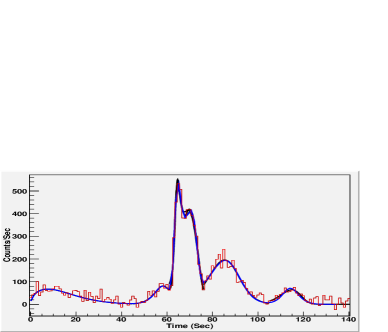
Figure 6.2: Multiple FRED profiles fitted 59-215 keV band RT-2/G background subtracted lightcurve (Time 0 means $T_{0}$ = 08h 28m 27s UT) for GRB 090618 (Rao et al. 2010b).

Table 6.1: FRED profile fitted results for RT-2/G lightcurves of GRB 090618

Pulse	Energy range (keV)	$F_{m}$ (s-1)	$t_{m}$ (s)	$r$ (s)	$d$ (s)	Width (s)
1		532.0	65.0	81.1	13.8	6.30
2	59-215	422.0	70.0	34.5	34	7.15
3		210.0	85.0	20.0	20.0	14.60
4		72.0	114.0	42.0	40.0	9.49
1		315.0	65	82.5	16.4	5.59
2	215-330	200.0	70.0	41.6	34.2	6.17
3		76	85.0	25.0	22.0	12.17
1	330-1000	144.0	65.0	78.3	22.5	4.77
2		64.0	70.0	88.0	84.0	2.93

$\bullet$ Spectral analysis results for GRB 090618

Figure 6.3: The unfolded $Swift$ BAT and $RT$-2/S combined energy spectrum of GRB 090618 (Rao et al. 2010b).

Spectral analysis for the GRB was done by using the RT-2/S and Swift BAT data. We used $15-200$ keV BAT, $100-210$ keV $RT$-2/S G1, and $250-650$ keV $RT$-2/S G2 data for our combined spectral fitting analysis. From our RT-2/S spectral data, we found the GRB peak energy at $\sim 180$ keV and total flux in $20-1000$ keV energy band is equal to $2.8\times 10^{-4}$ ergs/cm².

For RT-2 spectral data fitting we first generated response matrix using FTOOLs genrsp task. The GRB spectrum can be well fitted with the double power-law model introduced by Band et al. (1993). In this model, two power-laws join at break frequency $(\alpha-\beta)$E_p, where $\alpha$ and $\beta$ are the first and second power-law indices respectively. Figure 6.3 shows the unfolded power-law model fitted $Swift$ BAT and $RT$-2/S combined energy spectrum of the GRB 090618.

B. GRB 090820

The Fermi Gamma-Ray Burst Monitor (GBM) first detected the GRB 090820 by its trigger number 272421498 (Connaughton V. 2009) on 20th August, 2009 at 00:38:16.19 UT. The source location was at RA(J2000) = 87.7 degrees (5h 51m) and Dec(J2000) = 27.0 degrees ($+27^{\circ}0^{{}^{\prime}}$). The lightcurve of this bright GRB shows GBM triggered on a weak precursor, followed by a bright pulse beginning 30 sec later and lasting a further 30 seconds.

Both the RT-2 phoswich detectors (RT-2/S & RT-2/G) have detected this bright astrophysical event (Chakrabarti et al., 2009d). The satellite was in the GOOD/LIGHT mode with Earth latitude = $-64.09$ and longitude = $169.11$ with 600 sec duration of GOOD time observation, starting at 00h 29m 16sec (UT) and ending at 00h 39m 16sec (UT). After 30 sec, the satellite completely entered into the BAD mode of high charge particle region.

Figure 6.4: (a,b) Light curves in different energy band (marked) of (a) RT-2/S and (b) RT-2/G detectors. Emission peaks along with the weak precursor trigger pulse at T₀ = 00h 38m 16s UT are shown (Chakrabarti et al., 2009d).

The GRB lightcurve shows a simple profile of a strong emission peak at T₀+34 sec with a weak precursor (T₀ = 00:38:16 UT). The time duration of the brightest emission is around $19$ sec with $\sim 1100$ counts/sec.

Both RT-2/S and RT-2/G detectors have registered this burst profile in the energy band of $15-1000$ keV with the strongest emission in the energy range of around $100$ keV to $330$ keV. It is also noted that the burst width decreases with the increase in the energy band.

C. GRB 090926A

The very bright GRB 090926A was first detected by the Fermi-GBM trigger 275631628 (Bissaldi 2009) on 26th September, 2009 at 04:20:26.99 UT. The source location was at RA(J2000) = $354.5$ degrees (23h 38m), DEC(J2000) = $-64.2$ degrees ($-64^{\circ}12^{{}^{\prime}}$), with an uncertainty of $1^{\circ}$. The GBM lightcurve consists of single pulse with a duration (T90) of 20 s (8-1000 keV).

Figure 6.5: (a,b) Light curves in different energy band (marked) of (a) RT-2/S and (b) RT-2/G detectors. Two emission peaks along with the weak precursor trigger pulse at T₀ = 04h 20m 27s UT are detected in a wide energy band of 15 - 1000 keV (Chakrabarti et al., 2009e).

RT-2 instruments (RT-2/S & RT-2/G) also has detected this bright GRB at T₀ = 04h 20m 27s (UT) (Chakrabarti et al., 2009e). The satellite was in the LIGHT mode (pointing towards the Sun) for a short duration at a high latitude in its orbit. During this time, the GOOD time (away from the polar and SAA regions) observation was for 348 sec starting at 04h 16m 55sec (UT) and ending at 04h 22m 43sec (UT). This burst was also detected by KONUS-RF, another instrument onboard C ORONAS-PHOTON satellite (Golenetskii et al., 2009b).

The burst lightcurve consists of multiple peaks of total duration of $\sim 17$ sec, followed by a weak tail ending at T₀+30 sec. The strongest peak count rate is $\sim 1200$ counts/sec.

Both RT-2/S and RT-2/G detectors have registered the burst profile of this bright GRB in the energy band of 15 - 1000 keV with strongest emission in 60 - 215 keV energy band.

D. GRB 090929A

The Fermi Gamma-Ray Burst Monitor first reported the GRB 090929A by its trigger $275891585$ (Rau, A., 2009). The event occurred at 04:33:03.97 UT on 29th September, 2009 in the sky location of RA(J2000) = 51.7 degrees (03h 27m), DEC(J2000) = -7.3 degrees ($-7^{\circ}18^{{}^{\prime}}$), with an uncertainty of 1.3 degrees.

Figure 6.6: (a,b) Light curves in different energy band (marked) of (a) RT-2/S and (b) RT-2/G detectors. Emission peaks along with the weak precursor trigger pulse at T₀ = 04h 33m 04s UT are detected in a wide energy band (Chakrabarti et al., 2009f).

Both the phoswich detectors (RT-2/S & RT-2/G) of the RT-2 Experiment, has also detected this GRB (Chakrabarti et al., 2009f). During the time of GRB, the satellite was in the LIGHT mode (pointing towards the Sun) with GOOD time (i.e., away from the polar charge particle and SAA regions) observation of 1537 sec starting at 04h 21m 20sec (UT) and ending at 04h 46m 57sec (UT). This burst is also detected by KONUS-RF (Golenetskii et al., 2009c).

The burst lightcurve (1 sec bin) shows double peak profile of a total duration of just around 5 sec. The strongest peak count rate is $\sim 310$ counts/sec.

Both RT-2/S and RT-2/G detectors have registered the prompt emission from the GRB090929A in the energy band of 60 - 1000, with strongest emission in 60 - 215 keV energy band.

Chapter 6 ABBREVIATIONS

2D	Two Dimensional
3D	Three Dimensional
$\dot{A}$	$\dot{A}$ngstrom, $1\times 10^{-8}~{}cm$
A & A	Astronomy & Astrophysics
ACE	Advanced Composition Explorer
ADC	Analog to Digital Converter
ADAF	Advection Dominated Accretion Flow
AGN	Active Galactic Nuclei
AIP	The American Institute of Physics
al.	all
Al	Aluminium
ALEXIS	Array of Low Energy X-ray Imaging Sensor
ANS	Astronomical Netherlands Satellite
APPIDS	APPlication IDS
APJ	Astro-Physical Journal
AR	Angular Resolution
ASCII	American Standard Code for Information Interchange
ASI	Astronomical Society of India
ASIC	Application-Specific Integrated Circuit
ASM	All Sky Monitor
ASTROSAT	Indian Multi-wavelength ASTROnomy SATellite
AU	Astronomical Unit, $1.495\times 10^{13}~{}cm$ (Distance between Earth & Sun)
bb	black body
BASI	Bulletin of Astronomical Society of India
BAT	Burst Alert Telescope
BH	Black Hole

BHC	Black Hole Candidate
c	Velocity of light in vacuum, $2.99\times 10^{10}~{}cm~{}s^{-1}$
∘C	degree centigrade
CAM	Coded Aperture Mask
CB	Cannonball
CCAFS	Cape Canaveral Air Force Station
Cd	Cadmium
CENBOL	CENtrifugal pressure supported BOundary Layer
CERN	European Council for Nuclear Research
CGRO	Compton Gamma-Ray Observatory
cm	centimeter
CME	Coronal Mass Ejection
CMOS	Complementary Metal Oxide Semiconductor
CompST	Sunyaev-Titarchuk Comptonization model
CONFIG	CONFIGuration
CORONAS	Complex ORbital Observations Near-earth of Activity of the Sun
Cs	Cesium
CsI	Cesium Iodide
CSIR	Council for Scientific and Industrial Research
CZT	Cadmium Zinc Telluride
DC	Direct Current
DEC	DEClination
diskbb	disk black body
DOF	Degrees of Freedom
EA	Event Analyzer
EDS	Experiment Data System
e.g.	exempli gratia (for example)
EM	Emission Measure
ESA	European Space Agency
ESRO	European Space Research Organization
et	etc., excetera
EUV	Extreme Ultraviolet
eV	electron Volt, $1.6\times 10^{-12}~{}erg$
Exp. Astron.	Experimenal Astronomy
FB	Fireball
Fe	Iron
f-f	free-free
FFT	Fast-Fourier Transformation
FITS	Flexible Image Transport System
FMI	FITS Master Index
FOM	Figure Of Merit
FOV	Field Of View

FPGA	Field Programmable Gate Array
FRED	Fast Rise Exponential Decay
FWHM	Full Width at Half Maximum
FZP	Fresnel Zone Plate
g	gram
G	Gravitational constant, $6.672\times 10^{-8}~{}dyn~{}cm^{2}~{}g^{-2}$
ga	gaussian
GBM	Gamma-ray Burst Monitor
Gd	Gadolinium
GEANT4	GEometry ANd Tracking-4 (CERN particle simulation software 4)
GGS	Global Geospace Science
GOES	Geostationary Operational Environmental Satellites
GRB	Gamma Ray Burst
GTI	Good Time Intervals
H	Hydrogen
HEAO	High Energy Astrophysical Observatory
HESS	High Energy Stereoscopic System
HEXTE	High-Energy X-ray Timing Experiment
HID	Hardness-Intensity Diagram
HMXB	High Mass X-ray Binary
HV	High Voltage
HR	Hertzsprung-Russell
I	Iodine
IACT	Imaging Air Cherenkov Telescope
ICSP	Indian Centre for Space Physics
ICTP	the Abdus Salam International Centre for Theoretical Physics
IDL	Interactive Data Language
IJP	Indian Journal of Physics
IMXB	Intermediate Mass X-ray Binary
INFN	National Institute of Nuclear Physics (Italy)
INTEGRAL	INTErnational Gamma-Ray Astrophysics Laboratory
IR	Infrared
ISM	Inter-Stellar Medium
ISRO	Indian Space Research Organization
LabVIEW	Laboratory Virtual Instrumentation & Engineering Workbench
LC	Light Curve
LEO	Low Earth Orbit
LLD	Lower Level Discriminator
LMXB	Low Mass X-ray Binary

$k$	Boltzmann Constant, $1.38\times 10^{-16}~{}erg~{}K^{-1}$
K	Kelvin
keV	kilo electron Volt
kg	kilogram
km	kilo meter
kpc	kilo parsec
m	meter
$M_{\odot}$	Solar Mass, $1.989\times 10^{33}$ g
$M_{E}$	Earth Mass, $5.976\times 10^{27}$ g
$M_{Moon}$	Moon Mass, $7.347\times 10^{25}$ g, ($0.0123\times M_{E}$)
MC	Monte Carlo
MeV	Mega Electron Volt
MHB	Modified Horizontal Bridgman
$\mu$	micro
MJD	Modified Julian Day
MK	Mega Kelvin
mlab	Microprocessor Laboratory (ICTP, Italy)
mm	millimeter
MPhei	Moscow PHysics-Engineering Institute
Na	Sodium
NaI	Sodium Iodide
NASA	National Aeronautics and Space Administration (USA)
ns	nano second
nT	nano-Tesla, $1~{}Tesla=10^{4}~{}Gauss$
O	Oxygen
OEBH	Observational Evidence of Black Hole
pc	parsec, $3.26$ light years ($9.46\times 10^{17}~{}cm$), $3.085\times 10^{18}~{}cm$
PCA	Proportional Counter Array
PCU	Proportional Counter Unit
PDS	Power Density Spectra
PHA	Pulse Height Analysis
Ph.D.	Doctor of Philosophy
PL	Power-Law
p-p	proton-proton
PRL	Physical Research Laboratory
PS	Pulse Shape
PSD	Pulse Shape Discriminator
PSF	Point Spread Function
POS	Propagating Oscillatory Shock
PSPC	Position Sensitive Proportional Counter
QPO	Quasi-Periodic Oscillation
QPP	Quasi-Periodic Pulsation
QUASAR	Quasi-Stellar Radio Source

$R_{\odot}$	Solar radius, $6.959\times 10^{10}$ cm
$R_{E}$	Earth radius, $6.3713\times 10^{8}$ cm
$R_{Moon}$	Moon radius, $1.737\times 10^{8}$ cm, ($0.273\times R_{E}$)
RA	Right Ascension
RHESSI	Reuven Ramaty High Energy Solar Spectroscopic Imager
RMS	Root Mean Square
RXTE	Rossi X-ray Timing Explorer
RT-2	Röntgen-2
S	Sulphar
SAA	South Atlantic Anomaly
SAC	Satellite Application Centre
SDD	Silicon Drift Detector
SFM	Solar Flare Mode
SolarMax	Solar Maximum Mission satellite
SOHO	Solar and Heliospheric Observatory
SQM	Solar Quiet Mode
SS disk	Shakura-Sunyav disk
SSC	Scanning Shadow Camera
SSW	Solar SoftWare
STEREO	Solar TErrestrial RElations Observatory
TCAF	Two Component Advective Flow
Te	Telluride
TIFR	Tata Institute of Fundamental Research
Tl	Thallium
TRACE	Transition Region and Coronal Explorer
V	Volt
VCO	Voltage Control Oscillator
VSSC	Vikram Sarabhai Space Centre
ULD	Upper Level Discriminator
URA	Uniformly Redundant Arrays
UT	Universal Time
UV	Ultraviolet
W	Watt
XMM-Newton	X-ray Multi-Mirror Mission - Newton
Zn	Zinc

References

- Abramowicz, M. A., Czerny, B., Lasota, J. P. & Szuszkiewicz, E., Astrophysical Journal, 332, 646 (1988)
- Aschwanden, M.J., Sol. Phys., 111, 113 (1987)
- Band, D., et al., Astrophysical Journal, 413, 281 (1993)
- Bailyn, C. D., Orosz, J. A., McClintock, J. E. & Remillard, R. A., Nature, 378, 157 (1995)
- Battaglia, M. & Benz, A. O., Astronomy Astrophysics, 456, 751 (2006)
- Bissaldi, E., GCN Circulars Archive, 9933 (2009)
- Belloni, T., Homan, J. & Casella, P., et al., Astronomy Astrophysics, 440, 207 (2005)
- Belloni, T., Soleri P. & Casella P. et al., Mon. Not. of Roy. Astron. Soc., 369, 305 (2006)
- Bondi, H., Mon. Not. of Roy. Astron. Soc., 112, 195 (1952)
- Brown, J. C. , Solar Physics, 18, 489 (1971)
- Cenko, S. B., Perley, D. A., &Junkkarinen, V., et al., GCN Circulars Archive, 9518 (2009)
- Chakrabarti, S. K., Theory of Transonic Astrophysical Flows, (World Scientific Publishing, Singapore) (1990)
- Chakrabarti, S. K. & Molteni, D., Astrophysical Journal, 417, 671 (1993)
- Chakrabarti, S. K. and Titarchuk, L., G., Astrophysical Journal, 455, 623 (1995)
- Chakrabarti, S. K., Mon. Not. of Roy. Astron. Soc., 283, 325 (1996a)
- Chakrabarti, S. K., Astrophysical Journal, 464, 664 (1996b)
- Chakrabarti, S. K., Astronomy Astrophysics, 351, 185 (1999)
- Chakrabarti, S.K. & Manickam, S. 2000, Astrophysical Journal, 531, 41 (2000)
- Chakrabarti, S.K., Acharyya, K. & Molteni, D., A A, 421, 1 (2004)
- Chakrabarti, S.K., Nandi, A. & Debnath, D., et al., Indian J. Phys., 79(8), 841-845 (2005)
- Chakrabarti, S.K., Nandi, A. & Debnath, D., et al., VI MQW Conf. Proc. (POS), 103 (2006a)
- Chakrabarti, S.K. & Mandal, S., Astrophysical Journal, 642, 49 (2006b)
- Chakrabarti, S.K., Debnath, D., Nandi, A. & Pal, P. S., Astronomy Astrophysics, 489, L41-L44 (2008a)
- Chakrabarti, S.K., Debnath, D. & Pal, P.S., et al., MG11 Conf. Proc. (World Scientific), 569 (2008b)
- Chakrabarti, S.K., Bhowmick, D. & Debnath, D., et al., OEBH Conf. Proc. (AIP), 1053, 409 (2008c)
- Chakrabarti, S. K., Dutta, B. G. & Pal, P. S., Mon. Not. of Roy. Astron. Soc., 394, 1463 (2009a)
- Chakrabarti, S.K., Palit, S. & Debnath, D., et al., Exp Astron, Vol 24, P109 (2009b)
- Chakrabarti, S.K., Palit, S., Nandi, A., Yadav, V. & Debnath, D., et al., 1st ICST Conf. Proc. (IEEE), (in press) (2009c)
- Chakrabarti, S.K., Nandi, A. & Debnath, D., et al., GCN Circulars Archive, 9833 (2009d)
- Chakrabarti, S.K., Nandi, A. & Debnath, D., et al., GCN Circulars Archive, 10009 (2009e)
- Chakrabarti, S.K., Nandi, A. & Debnath, D., et al., GCN Circulars Archive, 10010 (2009f)
- Chen, W., Shrader, C. R. & Livio, M., Astrophysical Journal, 454, 880 (1995)
- Connaughton, V, GCN Circulars Archive, 9829 (2009)
- Cui, W., Shrader, C. R. & Haswell C. A., et al., Astrophysical Journal, 535, L123-L127 (2000)
- Dar, A., & De Rújula, A., astro-ph:0008474 (2000)
- Dar, A., & De Rújula, A., Physics Reports, 405, 203 (2004)
- Dar, A., ChJAS, 6, 301 (2006)
- De Rújula, A., Phys. Lett., 193, 514 (1987)
- Debnath, D., Chakrabarti, S.K., Nandi, A. & Mandal, S., Bull. of Astron. Soc. of India, 36, 151 (2008a)
- Debnath, D., Nandi, A. & Chakrabarti, S.K., et al., ASI Conf. Proc. (Bull. of Astron. Soc. of India), p.82, 25S, 82D (2008b)
- Debnath, D., Nandi, A. & Chakrabarti, S.K., et al., OEBH Conf. Proc. (AIP), 1053, 171 (2008c)
- Debnath, D., Chakrabarti, S.K. & Nandi A., Astronomy Astrophysics, 520, 98 (2010a)
- Debnath, D., Nandi, A. & Rao, A.R., et al., Exp. Astron., (in press) (2010b)
- Debnath, D., Chakrabarti, S.K. & Pal, P.S., (In preparation) (2010c)
- Debnath, D., et al. (In preparation) (2010d)
- Debnath, D., Chakrabarti, S.K. & Nandi, A., (In preparation) (2010e)
- Duijveman, A., Hoyng, P. & Machado, M. E., Solar Physics, 81, 137 (1982)
- Ebisawa, K., Titarchuk, L. & Chakrabarti, S. K., PASJ, 48, 59 (1996)
- Fishman & Inan, Nature, 331, 418 (1988)
- Fleishman, G.D., Bastian, T.S., & Gary, D.E., Astrophysical Journal, 684, 1433 (2008)
- Foellmi, C., Depagni, P., Dall, T.S. & Mirabel, I.F. A A, 457, 249 (2006)
- Gehrels, N., Ramirea-Ruiz, E. & Fox, D.B., ARAA, 47, 567 (2009)
- Ghirlanda, G., Nava, L. & Ghisellini, G., arXiv:0908.2807, (2009)
- Goff, C. P., van Driel-Gesztelyi, L. & Harra, L. K., et al., AA, 434, 761 (2005)
- Golenetskii, S., Aptekar, R. & Mazets, E., et al., GCN Circulars Archive, 9553 (2009a)
- Golenetskii, S., Aptekar, R. & Mazets, E., et al., GCN Circulars Archive, 9959 (2009b)
- Golenetskii, S., Aptekar, R. & Mazets, E., et al., GCN Circulars Archive, 9968 (2009c)
- Goodman, J., Astrophysical Journal, 308, L47 (1986)
- Hjellming, R. M. and Rupen, M.P., Nature, 375, 464 (1995)
- Hudford, G. J, Schmathl, E. J. & Schwartz, R. A., et al., Solar Physics, 210, 61 (2002)
- Hudson, H. S., Solar Physics, 24, 414 (1972)
- Hynes, R.I., Steeghs, D. & Casares, J., et al., Astrophysical Journal, 583, L95 (2003)
- Hynes, R.I., Steeghs, D. & Casares, J., et al., Astrophysical Journal, 609, 317 (2004)
- Homan, J., Buxton, M. & Markoff, S. et al., Astrophysical Journal, 624, 295 (2005)
- Jakimiec, J. & Tomczak, M., arXiv:0908.0656 (2009)
- Jahoda, K., Swank, J.H. & Giles, A.B., et. al., Proc. SPIE, 2808, 59 (1996)
- Jakimiec, J. and Tomczak, M., arXiv:0908.0656 (2009)
- Jaroszyski, M., Abramowicz, M. A. & Paczyski, B., Acta Astr. 30, 1 (1980)
- Klebesadel, R. W., Strong, I. B. & Olson, R. A, Astrophysical Journal, 182, 85L (1973)
- Kocevski, D., Ryde, F., & Liang, E., Astrophysical Journal, 596, 389 (2003)
- Knoll, G. F., Radiation Detection and Measurement, Wiley, New York (1999)
- Kocevski, D., Ryde, F., & Liang, E., Astrophysical Journal, 596, 389 (2003)
- Kotoch, T.B., Nandi, A. & Debnath, D., et al., Exp. Astron, (in press) (2010)
- Kotov, Yu., Kochemasov, A. & Kuzin S., et al., 37th COSPAR Scientific Assembly, p.1596 (2008)
- Krucker, S., Battaglia, M. & Cargill, P. J., et al., Astronomy Astrophysics Rev., 16, 155 (2008)
- Kubota, A., Tanaka, Y. & Makishima, K., et al., PASJ, 50, 667 (1998)
- Levine, A. M., Bradt, H. & Cui, W., et al., Astrophysical Journal, 469 L33 (1996)
- Levinson, A. & Eichler, D. Astrophysical Journal, 418, L386 (1993)
- Lin, R. P., Krucker, S. & Hurford, G. J., et al., Astrophysical Journal, 595, L69-L76 (2003)
- Liu, Q. Z., van Paradijs, J. & van den Heuvel, E. P. J., Astronomy Astrophysics, 368, 1021 (2001)
- Makishima, K., Maejima, Y. & Mitsuda, K., et al., Astrophysical Journal, 308, 635 (1986)
- Mandal, S. & Chakrabarti, S. K., Astrophysical Journal, 710, L147, (2010)
- Markert, T. H., Canizares, C. R. & Clark, G. W., et.al., Astrophysical Journal, 184, L67 (1973)
- Markwardt, C. B. & Swank, J. H., ATel, 14, (2005)
- McClintock, J.E. & Remillard, R.A., astro.ph, 6213 (2003)
- Mészáros, P. & Rees, M.J., Mon. Not. of Roy. Astron. Soc., 257, 29 (1992)
- Miller, J. M., Fabian, A. C. & Reynolds, C. S, et al., Astrophysical Journal, 606, L131 (2004)
- Mitsuda, K., Inoue, H., Koyama, K. & Makishima, K., et al., PASJ, 36, 741 (1984)
- Miyamoto, S., Kimura, K. & Kitamoto, S., et al., Astrophysical Journal, 383, 784 (1991)
- Molteni, D., sponholz, H. & Chakrabarti, S. K., Astrophysical Journal, 457, 805 (1996)
- Morrison, R. & McCammon, D., Astrophysical Journal, 270, 119, (1983)
- Motta, S., Belloni, T. & Homan J., Mon. Not. of Roy. Astron. Soc., 400, 1603 (2010)
- Nakariakov, V.M., Melnikov, V.F., & Rerznikova, V.E., Astronomy Astrophysics, 412, L7 (2003)
- Nandi, A., Rao, A.R., Chakrabarti, S.K., Malker, J.P., Sreekumar, S. & Debnath, D., et al., 1st ICST Conf. Proc. (IEEE), (in press) (2009)
- Nandi, A., Palit, S. & Debnath, D., et al., Exp. Astron., (in press) (2010)
- Narayan, R. & Yi, I. Astrophysical Journal, 428, 13 (1994)
- Novikov, I.D. & Throne, K.S., blho. conf. proc., 343 (1973)
- Nowak, M. A., Wilms, J. & Dove, J. B., Astrophysical Journal, 517, 355 (1999)
- Nowak, M. A., Mon. Not. of Roy. Astron. Soc., 318, 361 (2000)
- Orosz, J. A. & Bailen, C. D., Astrophysical Journal, 477, 876 (1997)
- Paczyński, B. & Wiita, P. J., Astronomy Astrophysics, 83, 23 (1980)
- Paczyński, B., Astrophysical Journal, 308, L43 (1986)
- Paczyński, B., Astrophysical Journal, 494, L23 (1988)
- Piran, T., RMP, 76, 1143 (2005)
- Pal, P.S, Debnath, D. & Nandi, A., et al., ASI Conf. Proc. (Bull. of Astron. Soc. of India), p.83, 25S, 83P (2008)
- Palit, S., Chakrabarti, S.K. & Debnath, D., et al., OEBH Conf. Proc. (AIP), 1053, 391 (2008)
- Palit, S., Chakrabarti, S.K. & Debnath, D., et al., Exp. Astron., Vol 24, P109 (2009)
- Papadakis, I. E. & Lawrence, A, Mon. Not. of Roy. Astron. Soc., 261, 612 (1993)
- Rao, A.R., Naik, S., Vadawale, S.V. & Chakrabarti, S.K., Astrophysical Journal, 360, 25 (2000)
- Rao, A.R., Malkar, J.P., Hingar, M.K., Agrawal, V.K., Chakrabarti, S.K., Nandi, A. & Debnath, D., et al., GCN Circulars Archive, 9665 (2009)
- Rao, A.R., Malkar, J.P., Hingar, M.K., Agrawal, V.K., Chakrabarti, S.K., Nandi, A. & Debnath, D., et al., Astrophysical Journal, 714, 1142 (2010a)
- Rao, A.R., Malkar, J.P., Hingar, M.K., Agrawal, V.K., Chakrabarti, S.K., Nandi, A. & Debnath, D., et al., Astrophysical Journal, (in press), (2010b)
- Rao, A.R., Malkar, J.P., Hingar, M.K., Agrawal, V.K., Chakrabarti, S.K., Nandi, A. & Debnath, D., et al., Solar System Research (Submitted), (2010c)
- Rau, A., GCN Circulars Archive, 9962 (2009)
- Remillard, R.A., McClintock, J. E. & Bailyn, C. D., et al., Astrophysical Journal, 522, 397-412 (1999)
- Remillard, R. A., McClintock J. E. & Orosz, J. A. et al., Astrophysical Journal, 637, 1002-1009 (2006)
- Rothschild, R. E., Blanco, P. R. & Gruber, D. E., et al., Astrophysical Journal, 496, 538 (1998)
- Rybicki, G.B. & Lightman, A.P., “Radiative Processes in Astrophysics”, p. 162 (1979)
- Ryu, D., Chakrabarti, S.K. & Molteni, D., Astrophysical Journal, 474, 378 (1997)
- Saito, K., et. al., 2006, in POS, VIth MQW Conf. Proc., 93 (2006)
- Samimi, J., Share, G. H. & Wood, K., et al., Nature, 278, 434 (1979)
- Sarkar, R., Mandal, S., Nandi, A. & Debnath D., et al., ASI Conf. Proc. (Bull. of Astron. Soc. of India), p.83, 25S, 83S (2008)
- Sarkar, R., Mandal, S. & Debnath, D., et al., Exp. Astron., (in press) (2010)
- Schady, P., Baumgartner, W. H. & Beardmore, A. P., et al., GCN Circulars Archive, 9512 (2009)
- Shakura, N. I. & Sunyaev, R. A., Astronomy Astrophysics, 24, 337 (1973)
- Shaposhnikov, N. & Titarchuk, L. G., Astrophysical Journal, 643, 1098 (2006)
- Shaposhnikov, N., Swank, J. & Shrader, C. R., et al., Astrophysical Journal, 655, 434 (2007)
- Smith, D., Heindl, W.A. & Swank, J.H., Astrophysical Journal, 569, 362 (2002)
- Smith, D.M., Dawson, D.M. & Swank, J.H., Astrophysical Journal, 669, 1138 (2007)
- Sobczak, G.J., McClintock, J. E. & Remillard, R. A., et al. Astrophysical Journal, 520, 776 (1999)
- Sreekumar, S., Vinod, P., Samuel, E., Malkar, J.P., Rao., A.R., Hinger, M.K. & Debnath, D., et al., Exp. Astron., (in press) (2010)
- Strohmayer, T. E., Astrophysical Journal, 552, L49-L53 (2001)
- Sui, L., Holam, G. D. & Dennis, B. R., et al., Astrophysical Journal, 612, 546 (2004)
- Sunyaev, R.A. & Titarchuk, L.G., Astronomy Astrophysics, 86, 121 (1980)
- Tingay, S.J., Jauncey, D. L. & Preston, R. A., et al., Nature, 374, 141 (1995)
- Tomsick, J. A., ATel, 2384, 1T (2010)
- van der Klis, M., AN, 326, 798 (2005)
- Veroing, A. M. & Brown, J.C., Astrophysical Journal, 603, L117 (2004)
- Vignarca, F., Migliari, S. & Belloni, T., et al., Astronomy Astrophysics, 397, 729 (2003)
- Yamaoka, K., Sugizaki, M. & Nakahira, S., et al., ATel, 2380, 1Y (2010)
- Young, C.W., Spencer, C.L., Moreton, G.E., & Roberts, J.A., Astrophysical Journal, 133, 243 (1961)
- Yu, W., ATel, 2556, 1Y (2010)
- Zaitsev, V. V. & Stepanov, A. V., Soviet Astron. Letter, 8, 132 (1982)
- Zaitsev, V. V., Stepanov, A. V. & Chernov, G. P., Solar Physics, 93, 363 (1984)
- Zhang, B., & Mészáros, P., IJMPA, 19, 2385 (2004)
- Zhang, S. N., Wilson, C. A. & Harmon, B. A., et. al., IAU Circ., 6046 (1994)